Radiata pine yield models

R A DI ATA P I N E YI ELD MODELS

by 3.W. Leech

Thesis submitted for the degree of Doctor of Philosophy Australian National University

Statement of originality

The Generalized Least Squares technique reported in Appendix 6 of this thesis was developed by Dr. I.S. Ferguson. Apart from this, and uhere recognized, this thesis is my own work.

\

'

LO

W<^

—

Acknowledgements

This study was undertaken under the supervision of Dr0 I0S0 Ferguson and Dr* L 0T. Carron of the Department of Forestry, Australian National University. Their constructive criticism and support uas greatly appreciated. I am especially indebted to Dr. Ferguson for his help in making the Generalized Least Squares analysis possible, and to Hr. D 0A, Miles who wrote the program to carry out that analysis.

Assistance has also been received from Professors A. Brown,

P.Co Young and C.R. Heathcote, and Dr. S.R0 Wilson of the Australian National University, and Dr. A.M.W. l/erhagen of the CSIRO Division of Mathematical Statistics.

The continuing encouragement and help of Messrs. N.B. Lewis and A. Keeves of the Woods and Forests Department of South Australia is also gratefully acknowledged.

The study was supported by a Commonwealth Post-graduate Research Award with AMU supplement, and an allowance by the South Australian Government under its tertiary assistance scheme for full time post­ graduate education awards.

Abstract

Data from radiata pine stands in the south-east of South Australia were used to investigate various aspects of stand yield models with a view to establishing a satisfactory predictive model for use in South Australia. In the first phase of the analyses data from unthinned stands uere used with Ordinary Least Squares (OLS) techniques to invest­ igate various model structures that have been proposed in the past, to determine whether yield or increment was the better dependent variable, and to investigate conditioning through a known base point, defined as site potential, and taken as yield at age 10. The second phase extended these analyses to include investigation of the effects of thinning var­ iations and soil differences, and also investigated the use of the model both for other forest regions in South Australia and for second rotation stands. Because these analyses were statistically unsatisfactory

Generalized Least Squares (GLS) and Bayesian statistical methods were used in the third phase to develop a simple yield prediction model that is statistically sound. This technique offers considerable promise for future work.

The conditioned form of the Mitscherlich ormonomolecular model below was the most satisfactory yield prediction model developed for radiata pine stands in South Australia.

1 _ exp(-p(A - 10 expC-a^ )) ) 1 - exp(-p(l 0 - 10 expt-a^)) where

p = 0.05271 - 0.006484 ln(Y1 Q ) a1 = -0.003467 Y1Q

and where

Y^ = yield at age A A = age, and,

TABLE OF CONTENTS

Acknowledgements (i)

Abstract (ii)

TABLE OF CONTENTS (iii)

LIST OF TABLES (ix)

LIST OF FIGURES (x)

LIST OF APPENDICES • (xi)

I INTRODUCTION 1

II THE DATA 5

Management practice in South Australia 6

Permanent Sample Plots 9

VARIABLES 11

Yield 11

Age 12

Site potential 12

Stand density 14

Thinning 14

Soil 16

Form 16

Other sources of variation 17

(iv)

III STATISTICAL METHODS 19

Introduction 20

PROPERTIES OF ESTIMATORS AMD PREDICTORS 23

MISSPECIFICATION 25

Homogeneity of variance 25

Serial correlation 27

Normality 29

Rank 29

Measurement error 30

Structure 31

ESTIMATION 32

TESTING 34

Hypothesis testing 34

Testing the assumptions underlying the analysis 36

Testing predictions 37

Summary of testing procedure 38

II/ GROWTH AND YIELD MODELS 40

COMPARISON OF GROWTH AND YIELD MODELS 42

Graphical models 44

Polynomial 46

Grosenbaugh 47

Bertalanffy 48

Gompertz-Thomasius 54

Oohnson-Schumacher 55

55

Hugershoff-Bednarz 56

Summary 57

M EXPLORATORY ANALYSES OF DATA FROM UNTHINNED STANDS 60

( v )

DATA 61

SITE POTENTIAL 62

Conditioning 62

Model formulation 64

ANALYSIS 67

Form of the dependent variable 68

Single or two stage analysis 69

STRATEGY 70

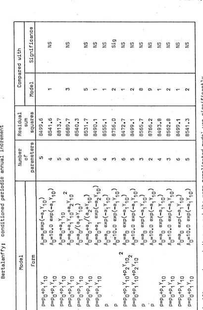
BERTALANFFY MODEL RESULTS 72

The evaluation of the general model 72 Periodic annual increment, conditioned 74 Periodic annual increment, unconditioned 78

Derivative 80

Yield, conditioned 82

Yield, two stage 83

Summary 86

00HNS0N-SCHUMACHER 87

Linear models 87

Nonlinear models, unconditioned 89

Nonlinear models, conditioned 91

Summary 93

BEDNARZ 94

OTHER MODEL FORMS 96

Gompertz 96

Polynomial 97

Lewis’s yield table 98

THINNING 102

Competition level 103

Thinning shock 107

Data 105

Analysis of competition level 110

Analysis of thinning shock 114

SOIL AND FORM 115

Data 117

Results 113

EXTENSION TO OTHER REGIONS 125

Upper south east 127

Adelaide Hills region 129

Northern region 130

Summary 131

SECOND ROTATION STANDS 131

SUMMARY 132

PART 2 GENERALIZED LEAST SQUARES ESTIMATION 134

VII MODELS FOR UNTHINNED STANDS 135

GENERALIZED LEAST SQUARES ANALYSIS 136

MODEL FORMULATION 137

ESTIMATION OF THE VARIANCE-COVARIANCE MATRIX 139

MODEL DEVELOPMENT 141

First stage models 141

Second stage models 143

Alternative error structures 145

Testing the model 148

Unconditioned model 151

l / m HOPELS FOR THINNED STANDS 152

FIRST STAGE HODELS 153

Formulation 153

Selection 154

BAYESIAN ESTIMATION 155

DATA 156

FIRST STAGE MODEL DEVELOPMENT 157

Thinning parameters 157

SECOND STAGE MODEL DEVELOPMENT 159

Site potential 159

Other variables 161

Alternative error structures 163

EXAMINATION OF THE DEVELOPMENTAL DATA 163 EXAMINATION OF THE INDEPENDENT TEST DATA 167

SUMMARY 171

(viii)

BIBLIOGRAPHY 179

APPENDICES 186

APPENDIX 1 DATA 187

APPENDIX 2 EVALUATION OF THE PARTIAL

DERIVATIVES 220

APPENDIX 3 SECOND LEVEL SERTALANFFY MODEL 224

APPENDIX 4 EXPLORATORY ANALYSES OF

UNTHINNED DATA 229

APPENDIX 5 ANALYSIS OF DATA FROM ALL

STANDS 240

APPENDIX 6 GENERALIZED LEAST SQUARES

ESTIMATION OF STAND YIELD

FUNCTIONS by

LIST OF TABLES

II.1 Relationship between site quality and site

potential 13

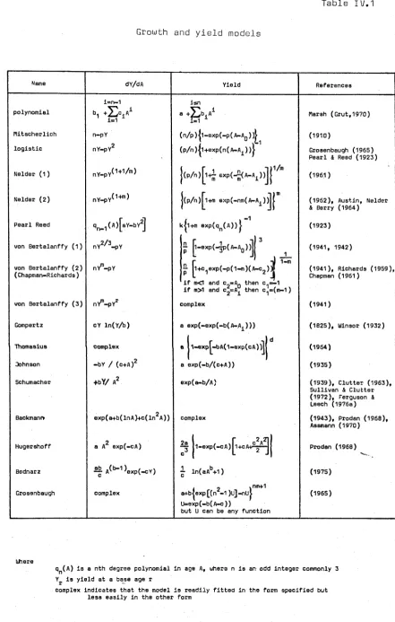
IV.1 Growth and yield models 45

V.1 Bertalanffy; conditioned periodic annual

increment 75

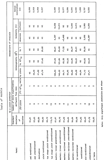
V. 2 Tests of models 77

V. 3 Oohnson-Schumacher; nonlinear 90

VI.1 Competition models 111

VI.2 Initial grouping of soil types 120

VI.3 final grouping of soil types 122

VI.4 Fit of Equation VI.9 to data from other areas 126

VI.5 Models for other areas 128

VII.1 Comparison of alternative unthinned models,

conditioned Bertalanffy 144

VII.2 Comparison of alternative unthinned models,

conditioned Bertalanffy, by soil type and forest 146 VII.3 Comparison of alternative error structures for

unthinned models 147

VIII. 1 Second stage models, posterior, conditioned

Bertalanffy 160

VIII.2 Second stage models, posterior, conditioned

Bertalanffy by soil type and forest 162 VIII.3 Second stage models, posterior, conditioned

Bertalanffy, comparison of alternative error

LIST OF FIGURES

( x )

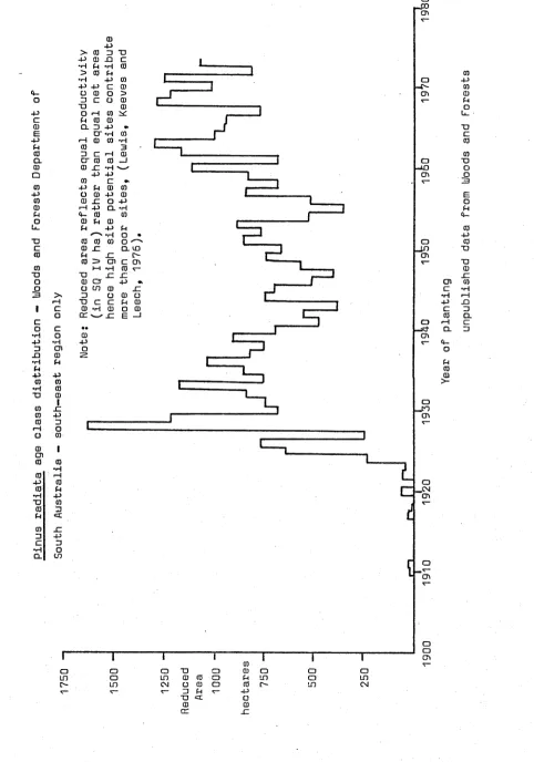
1.1 Pinus radiata age class distribution

-Woods and Forests Department of South Australia -

South east region only 3

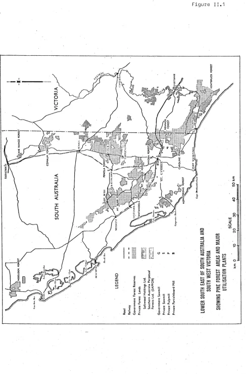
11.1 Hap of lower south-east of South Australia

and south-west Victoria 7

11.2 Hap of Forest Regions of South Australia 8 IV.1 Relationship between growth and yield 43 IV. 2 Proportion of asymptotic maximum yield that

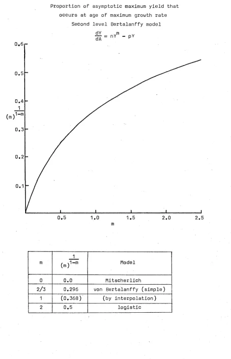
occurs at age of maximum growth rate, Second

level Bertalanffy model 53

V. 1 Bertalanffy two stage analysis, first stage

estimates and 95% confidence limits 85 VI. 1 Relationship between standing volume and volume

increment, and between standing basal area and

volume increment 104

VII. 1 Conditioned Bertalanffy model, First stage

estimates and 95%, confidence limits 142 VII.2 Estimated yield functions for developmental data 149 VII. 3 Estimated yield functions for selected independent

test data 150

VIII. 1 Conditioned Bentalanffy model, posterior, first

stage estimates and 95% confidence limits 158 VIII.2a Posterior; estimated yield functions for

developmental data 165

VIII.2b Posterior; estimated yield functions for

developmental data 166

VIII.3a Posterior; estimated yield functions for

test data 168

VIII.3b Posterior; test data

estimated yield functions for

APPENDIX 1 DATA 187

1.1 SUHHARY OF THE DATA BASE 188

1.2 SOIL TYPE 194

1 ,2a Key to soil type 195

1 .2b Summary by plots 196

1 .2c Notes on specific plots 199

1 .2d Occurrence of soil types by forest

district 200

1 .3 UNTHINNED STAND DATA 201

1.3a Plots in developmental and test

data ₂₀₂

1.3b Developmental data 203

1.3c Test data 204

1 .4 DATA FROH THE LOWER SOUTH-EAST 205 1 ,4a Developmental data by age and site

quality 208

1 ,4b Test data by age and site quality 209 1 .4c ' Developmental data by thinning 210

• CL Test data by thinning 211

1 ,4e Combined data by soil type 212

1 ,4f Second rotation plots 213

1.5 DATA FROH OTHER REGIONS 214

1.5a Noolcok and Cave Range data 215 1 .5b Adelaide Hills and Northern

regional data 216

1 .6 DATA FOR GLS ANALYSIS 217

1.6a Plots for prior estimate by soil

type and forest 218

APPENDIX 2 EVALUATION OF THE PARTIAL DERIVATIVES 220 2.0 Conditioned periodic increment model.

Residual sum squares for various

delta values 223

(xii)

APPENDIX 3 3.1 3.2 APPENDIX 4 4.1 4.2 4.3 4.4 4.5a 4.5b 4.5c 4.6a 4.6b 4.7

APPENDIX 5 5.1a 5.1b 5.1c 5.2 5.3

SECOND LEVEL BERTALANFFY HODEL 224 Integration of the second level

Bertalanffy equation to give a

yield equation 225

The limit form of the second level

Bertalanffy as m approaches 1.0 228

/

EXPLORATORY ANALYSES OF UNTHINNED

DATA 229

Analysis of trend in variance 230 Bertalanffy; general model 231 Bertalanffy; unconditioned periodic

annual increment 232

Bertalanffy; conditioned yield 233 Oohnson-Schumacher; linear

unconditioned 234

Oohnson-Schumacher; nonlinear

unconditioned 235

Oohnson-Schumacher; nonlinear

conditioned 236

Bednarz; conditioned yield 237 Bednarz; conditioned periodic

annual increment 238

Gompertz; conditioned yield 239

ANALYSIS OF DATA FROM ALL STANDS 240 Competition; reformulation of p 241 Competition; correction to increment 242 Competition; alternative indices 243

Thinning shock 244

( x i i i )

APPENDIX 6 GENERALIZED LEAST SQUARES ESTIMATION

OF STAND YIELD FUNCTIONS by

I I N T R O D U C T I O N

South Australia has little native forest and of necessity the

Government became interested in plantation forestry over a hundrea years ago, only 40 years after the state was first settled.

By 1920 the Woods and Forests Department realized that radiata pine, Pinus radiata (D.Don.), had the greatest growth potential of the species tried, and had developed a satisfactory silvicultural system for the management of the species. During the subsequent economic depression plantation establishment increased dramatically. The Department now controls some 76 700 ha of plantation of which 68 900 ha have been

planted with radiata pine. This resource is managed on an approximately 50 year rotation and has a comparatively even distribution of age classes as can be seen in Figure 1.1.

Prediction of future yield in South Australia is especially critical. Current prediction techniques (Lewis, Keeves and Leech, 1976) indicate that the increment of the resource is approximately equal to the commit­ ment to existing industry. The potential for expanding the area of plantations is very limited because of high land prices and the limited area of suitable soils, Moreover Keeves (1966) has shown that the second rotation on any site has, and will have, a lower yield than the first, so that future industry expansion is limited.

The objective of this study was to develop a yield prediction model for the radiata pine plantations in the lower south-east of South

Australia so that the Woods and Forests Department can continue to efficiently manage its plantation resource.

N o t e : R e d u c e d a r e a re fl e ct s eq u a l producti vit y ( i n S Q I V h a ) r a t he r t h a n e q u a l n e t a r e a 3

Figure 1,1

• H p -p 0 • H "D CO CO CO r-H u CD cn CO co -P co *H X) co p co n c • H CL P •P CO co 0 I JZ -p □ 0 CO 1 CO •H r-i CO P -P CO D <=c JZ -P n o CO 0 -p CJ HI JD c

•H ffl f-l -P 0 c 0 o > o 0 0 CO m -p •H 0 CO •H 3 i—1 0 CO _J •H s_/ -P C •> 0 0 -p 0 o -p CL -H 0 0 -P p

•H O • 0 O '--"N

CL UO

JZ o cn c cn •H 0

JZ JZ -p

0 JC

o 0 a

c p 0

0 o 0

JZ E _ i

_________ I o cn o -ID cn □ _!40 cn o cn CD _co cn

1 ~ T ~ ~ T ~ 1

0 ~ T ~ 1 ~ T ~

a o o "D CD 0 CD CD CD

in o m 0 0 CD p m CD in

o in CM U 0 O 0 c - m CM

^— ^— 3 p -P

TD cc o

Australia’s wood production obtained from coniferous plantations has in­ creased from 6% in 1950/51 to 18% in 1970/71 (Wilson, 1974) and the

F0RW00D Conferenca (Australian Forestry Council, 1974) predicted that the proportion will be some 57% by the year 2010, On the basis of the existing plantation resource alone radiata pine will become the major commercial forest type in Australia within a relatively few years.

The Mensuration and Management Research Working Group of the Stand­ ing Committee of the Australian Forestry Council discussed growth models for radiata pine at a meeting at Caloundra, Queensland, in 1974. The Group acknowledged that differences existed between regions within Australia in the growth of radiata pine, but the Group pointed out that a detailed analysis of the differences in growth and form between regions would lead to a better understanding of the species, and hence lead to better prediction models. The Group concluded that development of a generalized growth model which recognised such differences was both possible and highly desirable.

11 THE DATA

Management practice in South Australia Permanent Sample Plots

VARIABLES Yield Age

Site potential Stand density Thinning Soil Form

II THE DATA

South Australia is the driest state in Australia with only ,2% of

the area receiving more than 6C0 mm of rainfall per year (Bednall, 1957)*

Intensive forestry is necessarily limited to these higher rainfall areas,

the largest area of which is in the south-east of the state. The main

plantation resource in the lower south-east has been described by Bednall

(1957) and Douglas (1974), and consists of some 100 000 ha of softwood

plantations located in a compact unit as shown in Figure II.1. Some

61 000 ha are controlled by the Woods and Forests Department (Woods and

Forests, 1976), of which 55 400 ha have, been planted with radiata pine.

Elsewhere in the state the Woods and Forests Department has some

13 400 ha of radiata pine plantations, predominantly in five forest

reserves geographically separated from one another: Bundaleer and

Wirrabara Forest Reserves in the Northern region, and Mount Crawford,

Kuitpo and Second Valley Forest Reserves in the Adelaide Hills or Central

region (Figure II.2). Data from these areas were used to evaluate

whether the model developed using data from the lower south-east of the

state could be extended to other areas.

Management practice in South Australia

Current management practice in South Australia has recently been

described in detail by Lewis, Keeves and Leech (1976). However, some

features of current practice need to be reiterated here.

In South Australia radiata pine plantations are stratified into

volume productivity classes which are termed site quality classes,

volume being considered a more effective basis for stratification than

upper stand height (Keeves, 1970). Site quality assessment is based on

7

Figure 11.1

F i g u r e I I . 2

B o o lc u n d a F. R.

{/• Mt. B ro w n F. R.

W illow !«

NORTHERN

W lrra ba ra F. R.

■ Y arcow ie A B u n d ale e r F. R. le rb e rt F. R. C rysta l B ro ok F. R.

R e dh lll F. R. ton F. R.

WESTERN

B arun ga F. R.

M u rth o F. W a lka rle F. R.

f S M u n a l B a rrl F. P jy ^ M u n d ic F. F

>, t L y ru p F. R.

CENTRAL \

W1LL1AMSTOWN W /

MURRAY LANDS

Mt C raw fo rd

; M o n a rto C N u rse ry

MEADOW S

• j 4

K u ltp o F. R. J

-P arllla F. R. ^ TaUem B e n d F . R.

G ooli

SOUTH-EAST

N o o lo o k F. R.

WOODS AND FORESTS DEPARTMENT _{Cave Range F. R. ^}

C o m j'jm F. R. FOREST REGIONS OF SOUTH AUSTRALIA

P a ro le , F. R. Mt. B u rr F. R.

M IL U C fh T • . » T . . .

Ta nta no o la F^R V w \ \ Mt. G am bler F. R. #

MT QAMB1EA

K o n g o ro n g F. f i V ^

M

S

Inventory is carried out on a five yearly cycle using temporary 0*1 ha plots. The intensity of sampling is such that the average

logging unit of some 30 ha has five plots selected at random within site quality strata. In each plot diameters are measured and the trees to be removed during the next five year period are demarcated. Volumes

available from thinning are estimated using a tree volume equation, with appropriate adjustment for increment on the thinnings between time of inventory and the scheduled year of thinning (Leech, 1973),

A short term (five year) cutting plan is then produced, delineating where thinning and clear felling should be carried out. The inventory data and the cutting plan are also used to predict yield from the

resource some 60 years into the future, using a deterministic simulation model developed by the author. The model developed in this study is intended to replace the yield prediction model currently incorporated in that long term planning model.

Permanent Sample Plots

Following the first forest inventory in South Australia permanent sample plots were established in 1935 and these have been gradually augmented so that there are at present 313 plots in radiata pine plant­ ations in the south-east of the state, These plots have been remeasured at various intervals and provided the data base for this study.

Plots have generally been measured mere frequently for basal area and upper stand height than for volume, measurement frequency decreasing with increasing age, but have always been measured for volume at time of thinning. The thinning regime for each plot was prescribed at plot establishment, although some plots have been rescheduled to widen the range of treatments.

Mensuration practice has remained more or less constant since plots were first established and is described in detail elsewhere (Lewis, Keeves and Leech, 1976). However, two aspects of measurement have changed over time;

1 sampling for volume, and, 2 height estimation.

These were considered further to see whether the changes had any serious implications for this study.

Initially mean dominant height was estimated. The current defin­ ition of ’predominant height’ (Lewis, Keeves and Leech, 1976) has only been in use since 1952. This change has more serious consequences than those for volume because the differences betueen the two measures may be substantial. Estimates of predominant height were available for some plots prior to 1962 but their precision and bias were unknown. The estimates were considered satisfactory for the determination of form estimates but were considered unsatisfactory for the development of height prediction models.

11

VARIABLES

As in most studies of this kind spanning long periods of time, the data available dictate the variables which can be used in the model.

Yield

The objective of a yield model is to predict the utilisable volume of wood that can be taken from a site. The utilisable volume depends on the volume available and the volume lost or wasted in logging, and this loss or wastage varies considerably depending on the equipment used. However, this study is restricted to estimating the volume available. It is envisaged that separate studies will be carried out from time to time to determine or revise the volume lost or wasted in logging.

12

Age is generally considered to be the most important independent variable in growth and yield studies (Buckman, 1962) and was the only independent variable in many of the earlier models. In South Australia plantations are established in winter using one year old seedlings, however the age of the plantation is taken as the number of years since planting out, ignoring the period in the nursery. All permanent sample plot data were measured in the period between late Nay and early

September, with the measurement program starting in the same locality each year and progressing in the same sequence so that measurements in any plot were generally made in the same month each time. The seasonal

fluctuation in growth within each year (Pawsey, 1964) can therefore be ignored.

Site potential

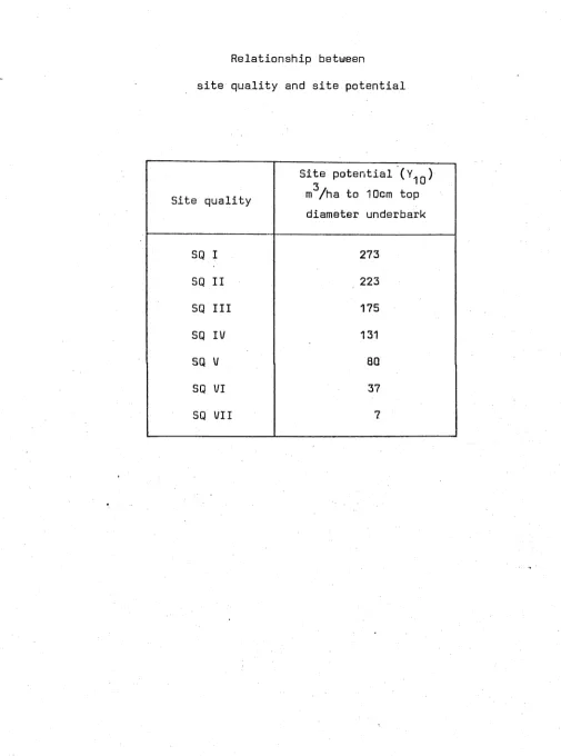
Site quality assessment is carried out in South Australia in the summer when the stand reaches age 9\ years, however, as the plots were all measured in winter the base age for this study was assumed to be 10 years. In this study the total volume yield underbark at age 10 years (Y^g) in cubic metres per hectare to a 10 cm top diameter was used as the definition of site potential. The relationship between site potential (Y^g) and site quality from the age 9^ assessment is shown in Table II.1.

For plots where there were no measurements at age 10, Y^g was estimated by linear interpolation, or if this was not possible, by

extrapolation. The extrapolation was based on the average of the first two volume increments available and was confirmed by comparing estimated Y^g with extrapolation using Lewis's yield table (Lewis, Keeves and

Leech, 1976), and by inspection of the basal area-age trend; many of the plots having been measured for basal area before volume measurement

13

Table II.1

Relationship between site quality and site potential

Site quality

Site potential (Y^g) m'Vha to 10cm top diameter underbark

SQ I 273

SQ II 223

SQ III 175

SQ IV 131

SQ V 80

SQ VI 37

14

commenced.

Stand density

Indices of stand density inevitably raise issues concerning definition and measurement (Leech, 1973), however in this study the choice of a variable to use as an index of stand density was restricted. There was no point in using indices based on such variables as standing basal area or upper stand height because such variables change contin­ uously with age and require a separate model to be developed for predic­ tion of future density. Only two of the variables available seemed appropriate, stocking and standing volume.

Stocking, the number of trees standing per hectare, has the advantage of being readily measured in the field, but is not entirely adequate as a index of density (Leech, 1973). Although not so easy to measure,

standing volume is measured on all permanent sample plots and can

readily be estimated for inventory plots. Standing volume seemed likely to provide a better index than number of trees so both these variables were tried in subsequent analyses.

Thinning

The description of a thinning regime can be separated into three parts (Lewis, 1959; Ford— Robertson, 1971).

1 Thinning type; indicating the categories of trees to be removed in the thinning based on size or crown classification.

15 3 Thinning interval; indicating at what stages in the development of

the stand these removals are to be made. This is generally expressed in years although it could be expressed in terms of volume or basal area growth since the last thinning.

The thinning type practised in South Australia has for many years been essentially a thinning from below with all suppressed and sub­

dominant trees being removed as well as a proportion of the co-dominants and dominants to help space the trees. Indices of thinning type are generally ratios of either mean tree diameter (Lewis, 1559; Braathe, 1957; Soergensen, 1957) or volume (Lewis, Keeves and Leech, 1975), of the trees removed from the stand to those either before or after

thinning. Within the available data the range of thinning type was quite narrow (if thinning type was defined as the ratio of the mean diam­ eter of thinnings to the mean diameter before thinning, the mean thinning type was 0.92 with a standard deviation of 0.04), and thus thinning type was not included as a variable in the subsequent analyses.

The grade of a thinning is a measure of the change in competition level due to that thinning. Grade is commonly specified in terms of either residual basal area (Gentle et al.t 1962; Robinson, 1968) or residual number of trees (Lewis, 1959, 1963) and in this absolute form is in essence an index of stand density which has already been discussed.

Buckman (1962) considered the more logical measure to be the proportion of the forest cut either as volume, basal area or number of trees per unit area. This relative form provides a measure of the shock that the stand has suffered in thinning and should obviously be based on the same variable as stand density.

16

practice generally keeps within one or two years of this ideal. Perm­ anent sample plots include a somewhat wider range of thinning interval than normal plantation practice.

Soil

The soils of the south-east region of South Australia have been described and typed by Stephens (Stephens et si., 1941) who conducted a detailed soil survey of much of the forest area. Three soil profiles have been described on all permanent sample plots and have been allocated to these soil types with three depth phases superimposed. For other regions the soil profiles were allocated to a soil type on the basis of a number of different surveys, but the soil types generally reflect morphological differences on a broader scale than the south-east survey.

Form

Uhen considering the possible effect of form on increment or yield the differences between form factor and taper need to be considered; both being related to different aspects of the concept of form. A number of alternative stand based indices of form were available based on standing basal area (m /ha) and a measure of upper stand height, predominant height (m). These indices are crude proxies for the more commonly used tree based indices, but were the best available,

1 Stand form factor, the ratio of standing volume to the product of basal area and predominant height.

2 Stand form factor at age 1G, possibly an indicator of differences between soil types or regions because it is unaffected by thinning and is age invariant.

17 4 Average stand taper, the ratio of mean tree diameter to predominant

height, mean tree diameter being the diameter equivalent to the mean basal area* This was considered more likely to vary between soil types than stand form factor as on some heavier soils higher than average basal area is accompanied by lower than average predominant height.

5 Average stand taper at age 10, possibly a better index than average taper because, as with form factor at age 10, it is age invariant and independent of thinning.

5 Relative stand taper, the ratio of average stand taper to average stand taper at age 10.

Where data at age 10 years were not available, interpolated or extrapolated figures were used.

Other sources of variation

18

Variables reflecting man-made influences such as nutrition and tree breeding were not available in a form suitable for inclusion in these analyses. This is clearly an area which warrants urgent attention in the future, since future yields will be affected by these influences. However, their omission was not critical to this study as the bulk of the present plantation estate was not established from seed orchard stock and has not received intensive treatment with fertilizers.

THE DATA BASE

The data were extracted from manually maintained permanent sample plot registers and files and were coded for punching onto cards. After the data were punched and verified a program developed by the author was used to check the data as rigorously as possible, finally producing appropriately formatted data files and a facsimile of the register. Painstaking reconciliation of this register with the manually maintained register, resolving any remaining sources of difference or ambiguity, ensured that the data were as error free as possible.

The data were largely measured in imperial units, the conversion to metric being made in 1973. The data base thus included metric measure­ ments and metric conversion of imperial measurements, but careful check­ ing reduced potential errors from this source to a minimum.

The data are summarised in a number of tables in Appendix 1• Appendix 1.1 summarises the complete data base, Appendix 1.2 the soil types, and Appendices 1,3 to 1.6 the different data sets used during

Ill STATISTICAL METHODS Introduction

PROPERTIES OF ESTIMATORS AND PREDICTORS MISSPECIFICATION

Homogeneity of variance Serial correlation Normality

Rank

Measurement error Structure

ESTIMATION TESTING

Hypothesis testing

Testing the assumptions underlying the analysis Testing predictions

III STATISTICAL METHODS

Introduction

The estimation of the relationship between one variable and a

number of others is a common problem in forestry and is generally

accomplished by the use of multiple linear regression analysis using

the O r d i n a r y Least S q u a r e s ’ (OLS) technique. Multiple regression

requires a model with a linear structure, the linearity referring to

the coefficients or parameters of the independent variables,

j=k

yi =

Z

-j=1

where

b . J

e .

l

n

k

is the i'th observation of the dependent variable,

( i = 1 .... n),

is the i ’th observation of the j ’th independent variable

( i = 1 .... n, j = 1 ... k),

is the j ’th parameter to be estimated, ( j = 1 . ,..,k ),

is the error term for the i ’th observation,

is the number of observations, and,

is the number of parameters.

9

The linear model can be stated in matrix form as

21

where

e n

Linearity is often too restrictive a requirement and models with a nonlinear structure may need to be examined. The general form of a nonlinear model can be represented thus:

V = f(B,X) + E (III.3)

where the f operator is used to denote a function nonlinear

in the parameters B, and where the notation is as for Equation III.2,

Sometimes a nonlinear model can be transformed (for example by taking logarithms) to obtain a form which is linear in the parameters. These intrinsically linear models, to use Draper and Smith's (1966) terminology, can be estimated in the transformed state using OLS.

In general, however, DLS cannot be used to estimate the parameters of nonlinear models. The normal equations which result from different­ iating the objective function are not linear in the unknown parameters, and no exact analytical solution for these equations exists. An

iterative approximate solution must be employed. Even so, there is no single algorithm which will unfailingly yield satisfactory estimates of the parameters of nonlinear models.

23

PROPERTIES OF ESTIMATORS AND PREDICTORS

The f o l l o w i n g p r o p e r t i e s ( K e n d a l l and S t u a r t , 1 9 5 1 ; G r a y b i l l ,

1 9 6 1 ; U c n n a c o t t and U o n n a c o t t , 1 9 7 0 ) a r e g e n e r a l l y s o u g h t f o r l i n e a r

e s t i m a t o r s :

An e s t i m a t o r s h o u l d be u n b i a s e d . An u n b i a s e d e s t i m a t o r i s one

t h a t on a v e r a g e h a s t h e same v a l u e as t h e t r u e e s t i m a t o r . For

e x a m p le b . i s an u n b i a s e d e s t i m a t o r o f b . i f

J J

E(V

w h e r e

E i s t h e e x p e c t e d v a l u e o f t h e p a r a m e t e r .

B i a s i s d e f i n e d as

Bl

b . J

E ( b . ) - b .

J J

w h e r e

( I I I . 5 )

Bl i s t h e b i a s o f t h e p a r a m e t e r b . ,

bj

J

An e s t i m a t o r s h o u l d be e f f i c i e n t . liJhen c o m p a r i n g tw o a l t e r n a t i v e

/— ^

e s t i m a t e s o f b b . and b . t h e n t h e m o s t e f f i c i e n t e s t i m a t o r i s t h e

J J J

o n e w i t h t h e l o w e r v a r i a n c e . The r a t i o o f t h e v a r i a n c e s p r o v i d e s

a m e a s u r e o f t h e r e l a t i v e e f f i c i e n c y i f t h e e s t i m a t o r s a r e u n b i a s e d .

The r e l a t i v e e f f i c i e n c y o f b . c o m p a re d w i t h b . i s :

ö

V

R =■ ---

J-cfS.

w h e r e

R i s t h e r e l a t i v e e f f i c i e n c y , a n d ,

(T i s t h e v a r i a n c e o f t h e e s t i m a t o r b ., ^ c . x T b . .

i J

The m o s t e f f i c i e n t e s t i m a t o r i s t h e m inimum v a r i a n c e e s t i m a t o r as by

d e f i n i t i o n t h e r e c a n be no e s t i m a t o r u i t h a g r e a t e r r e l a t i v e e f f i c ­

3 An estimator should be consistent. Estimators are said to be consistent if

- b^)2— > 0 (III.7)

and as

- b )2 = b| + CT b. (III.8)

J J j J

an estimator b . is consistent if J

Lim Bgv = 0 (III.9)

j n — >oo

2

Lim 6 b = 0 (III.10)

n— > oo

If only the bias approaches zero then the estimators are said to be asymptotically unbiased, but not strictly consistent.

4 An estimator should be sufficient. An estimator is said to be sufficient if it contains all the information in the set of obser­ vations regarding the parameter tü be estimated (Fisher, 1921, 1925; Deutsch, 1965).

OLS estimators possess these properties provided that the data and model conform with the assumptions underlying Classical normal linear regression’, to use Goldberger’s (1964) terminology. Under these con­ ditions OLS estimators are also identical to the maximum likelihood estimators. OLS estimators also provide predictors which are best (i.e. minimum variance) linear unbiased predictors (Theil, 1971).

For nonlinear models with independent, normal and identically

25

errors of estimation which may be introduced through the iterative approximate process of solution. Thus the properties of predictors based on small-sample OLS estimators of nonlinear models are not well defined.

MISSPECI FICATION

The assumptions underlying the use of OLS estimation for classical normal linear regression models are as follows (Goldberger, 1964):

1 The variance should be homogeneous over the range of the dependent variable.

2 The error terms should be independent of one another.

3 The error terms should be normally distributed.

4 The rank of the matrix of observations should be equal to the number of parameters to be estimated and less than the number of observations.

5 The variables should be measured without error.

6 The model should have the correct structure and include all the relevant variables, but no others.

If OLS estimation methods are used for a model that is misspecified in terms of these assumptions then the estimates may be biased, in­

efficient and/or inconsistent depending on the form of the misspecification, as the following sections indicate.

Homogeneity of variance

e(e&') = <52 i (iii.li)

where

I is the identity matrix of order rvyn ,

E is the error of the i observations, and,

'V 7 7

2

(T is the variance.

If this assumption is violated then the estimators are unbiased but inefficient (Johnston, 1963).

To test the variance for homogeneity the data are generally

partitioned and the variance of each cell calculated. There is general agreement (Sokal and Rohlf, 1969; Acton, 1959) that Bartlett’s test of homogeneity (1937) is better than either Hartley’s (1950) or Cochran’s (1941) test although Acton considers that none of these tests is robust, all being sensitive to non-normality in the underlying distribution.

Heterogeneity seemed most likely to arise between different plots, and within any one plot the variance might also increase with increasing age or with decreasing site potential. As insufficient data were

available to test for heterogeneity by age within plots, the first test was by plots alone. The data were then pooled and partitioned into age and site potential cells and the cell variances tested for heterogeneity. As a third test the data were ordered on the expected value of the

dependent variable and divided into approximately equal cells in a general omnibus test for all other possible sources of heterogeneity.

To overcome heterogeneity, observations are generally weighted by the reciprocal of the square root of the estimated variance (Cunia, 1964;

of the estimation technique.

Serial correlation

The error term in the linear model is assumed to be unbiased,

that is

E(ei ) = 0 (III.12)

and as well the error terms are assumed to be independent of one another

(Kendall and Stuart, 1961; Graybill, 1961).

E(e e ) = 0 for a11 1 (III.13)

If the latter assumption is violated then the OLS estimators will be

inefficient (Johnston, 1963).

Serial correlation most commonly occurs in time series due to

mis-specification either by omitting variables (Ulonnacott and Wonnacott,

1970) or by selecting the wrong model structure (Cochrane and Orcutt,

1949). Errors in the data are another possible source of serial

correlation (Cochrane and Orcutt, 1949) but these seemed unlikely to be

of importance in this study. As noted earlier the data for this study

were all collected at the same time of the year thus eliminating one

source of seasonally induced serial correlation.

The most commonly used test for serial correlation is that of

Durbin and Watson (1950, 1951).

The statistic is

i=n 2

£ (

-

d =

i = I

where

n is the number of observations, r

e^ is the error of the i ’th observations, and,

27

This test in its original form is not an exact test but provides upper and lower bounds to an inconclusive zone for from 15 to 100 observations. Because it is not an exact test a number of authors have developed nom­ inally exact tests of which the one by Theil and Nagar (1961) is probably the most commonly usedc In their latest paper Durbin and Watson (1971) concluded that many of these exact tests are "too inaccurate for practical use", and further refined an approximation they had suggested in their earlier papers. However, this also seemed inappropriate for this study.

In this study the number of observations from each plot was limited to 16 or fewer, generally 10-13. Although serial correlation was

29

Normality

Uhen making inferences about model structure using statistical tests of hypotheses the error term is assumed to be normally distributed.

Normality could be tested using the Chi-square statistic, but this test is not specific in that it fails to indicate whether skewness or kurtosis is the problem. To overcome this problem Sokal and Rohlf (1969) and Snedecor and Cochran (1967) describe techniques for estimating moment statistics of skewness and kurtosis. These two statistics are then compared with t (two tailed) for infinite degrees of freedom. The Shapiro-U/ilk statistic (Shapiro and Ulilk, 1965) is more powerful

(Shapiro, Wilk and Chen, 1968) than these other statistics but the tests of relative power indicated little gain when the number of observations increased past 50.

Tests of normality could not be carried out by plots because there were too few observations even for the Shapiro-liiilk test. For the pooled data there were more than 100 observations and in these cases the

Shapiro-liiilk test is difficult to apply and perhaps even dangerous ( D ’Agostino, 1971). The moment statistics were therefore selected as the test statistics because they indicated the type of departure from normality and were relatively powerful for the sample sizes used in this study.

Rank

In general, these assumptions are easily met by careful definition and selection of the set of independent variables* However, marked collinearity between any two independent variables gives rise to

parameter estimates with very high sampling errors. Thus this condition also needs to be avoided.

Measurement error

OLS assumes that the variables are measured without error (Kendall and Stuart, 1961; Ulonnacott and Ulonnacott, 1970)* If the dependent variable is measured with error, but the error is unbiased, then the variance of the error term for the model is inflated accordingly.

This problem is therefore of comparatively little concern, although the increase in the error variance may obscure relationships between the dependent and independent variables.

Errors of measurement in the independent variables may give rise to more serious problems unless;

1 the errors are unbiased, and,

2 the data to be used in subsequent prediction are measured in the same way as those used to estimate the parameters.

Under these circumstances OLS estimators will give unbiased predictions (Ulonnacott and UJonnacott, 1970), even though the estimators are biased relative to those appropriate to the independent variables when measured without error.

The measurement practice used in the development of the data base has been described by Lewis, Keeves and Leech (1976) and in part by

Structure

There are three main forms of structural misspecification: 1 choosing the wrong model structure, for example by using the

logarithm of the dependent variable where that transformation is inappropriate to the model,

2 omission of an explanatory independent variable, and, 3 inclusion of independent variables that are irrelevant.

The first type of structural misspecification can obviously lead to an inefficient prediction model even though the estimators themselves are efficient.

If relevant independent variables are omitted, either by mistake or because data are not available, then the estimates of the remaining parameters are likely to be biased and inefficient (liJonnacott and liionnacott, 1970).

If irrelevant independent variables are included then the estimators should be unbiased, but they will be inefficient because there are fewer degrees of freedom in the residuals used to estimate the variance.

Because of the ’noisy’ parameters the model is likely to be an erratic predictor, especially when used outside the range of the original data.

ESTIMATION

Estimation of the parameters of linear models is relatively simple because an analytical solution exists (Kendall and Stuart, 1961; Theil, 1971; Draper and Smith, 1966), Algorithms which incorporate this technique have been implemented in a number of computer programs for multiple regression analysis and two well-known programs REX (Grosen- baugh, 1967) and SPSS (Nie et al,t 1975) were used in this study.

For nonlinear models the objective function cannot be minimized analytically and a number of alternative algorithms (Goldfeld and Quandt, 1972; Sadler, 1975) have been developed to approximate the minimization iteratively.

The algorithms commence from feasible starting values for the parameters and aim to reduce the objective function by successively changing the parameter values until a minimum is reached.

There is no certainty that a particular algorithm will be satisfac­ tory for all models and all data sets, Goldfeld and Quandt (1972) investigated a number of alternative algorithms, testing them against different models and data sets in an effort to compare their effective­ ness, No one algorithm was the most efficient for all the examples, but two particular algorithms performed consistently well. Refined versions of these algorithms are implemented in a nonlinear parameter estimation program developed by Bard (1967); the Gauss-Newton method (Eisenpress and Greenstadt, 1966; Carroll, 1961), and the Davidon- Fletcher-Powell method (Fletcher and Powell, 1963; Sadler, 1975).

As the algorithms are iterative it is necessary to use terminating criteria to stop computation at an appropriate end point. Three

33

The change in the parameter estimates between successive iterations should be within a preset tolerance.

i

< di (

In this criterion (Marquardt, 1963) d^ is the desired tolerance for the parameter and d^ ensures that if the estimated parameter is close to zero then computation will stop. Setting

d^ = 0.00001 and d^ = 0.001 has been found to work well in practice (Marquardt, 1963).

2 The relative change in the objective function between iterations should also be within an arbitrary tolerance, commonly Marquardt’s criterion. This is especially useful when the response surface of the objective function is relatively flat for changes in the parameters,

3 The number of iterations should be less than an arbitrary

maximum so that if the other criteria fail because the algorithm cannot converge that particular model then computation will cease.

To ensure that the algorithm has converged, that is, a true minimum has been reached (a stationary minimum, but not necessarily a global one), the Hessian matrix (matrix of second order derivatives of the function) should be positive definite (Morrison, 1976). There is no guarantee that the minimum is a global one, but careful specifica­ tion and testing of the model can reduce any doubt in this regard.

The nonlinear parameter estimation program of Bard (1967) uses Marquardt's (1963) criterion for convergence and orovides information sufficient to show whether or not the Hessian matrix is positive

A user supplied subroutine is required to evaluate the function and its partial derivatives. For most growth models the partial derivatives are complex so an additional subroutine was developed to evaluate the partial derivatives numerically. This reduced the com­ plexity of the programming changes necessary between models. The technique adopted is detailed in Appendix

2-TESTING

Three different types of tests were used in this study:

1 Hypothesis tests to determine whether one model is better than another or to determine whether a model is internally consistent.

2 Tests of the assumptions underlying the model.

3 Tests of the model as a predictor.

Hypothesis testing

In developing a satisfactory model it was necessary to discriminate between models and between alternative forms of each model by testing a null hypothesis against its alternative (Johnston, 1963; Draper and Smith, 1966; Wonnacott and Uonnacott, 1970). Two important considera­ tions in deciding how the alternative hypotheses should be tested were 1 the choice of the test statistic, and,

2 the choice of the significance level.

For nonlinear models the situation is not so clear cut. As noted

earlier the small-sample properties of OLS estimators of nonlinear models

are not well established, Moreover, estimates of the precision of the

parameter estimates are generally based on a linear approximation, which

may or may not be sufficiently accurate (Guttman and Fleeter, 1965),

depending on the particular form of the model and the characteristics

of the surface of the likelihood function.

Nevertheless Gallant (1975), who studied models similar in form to

those of interest in this study, recommended the use of a test statistic

C, analogous to the use of the F statistic in analyses of variance for

linear models.

c = CT^ / a 2 ( I I I . 15)

2 2

where (T ^ and (7 ^ denote the maximum likelihood estimates of the

variance of the respective error terms in the two alternative

2 2

models,

CT > (T , .

The statistic is tested against the critical values of the

statistic C*.

C* = 1 - i Fp / (n - j)

where

F = P

i =

j =

n =

A av * ets jP f 0 * r

upper 100p^ points of an F distribution,

number of parameters of interest,

the total number of parameters, and,

the total number of observations.

( III.16 )

Again, following G a l l a n t ’s (1975) work, the (approximate) t stat­

istic was used to test hypotheses regarding the inclusion or otherwise

of individual parameters in a particular model.

Tests of hypotheses involving disparate families of both linear and

nonlinear models we-re achieved by comparing the predictive properties of

than the complex tests of Cox (1961, 1962).

The level of significance to be used in hypothesis testing must also be carefully considered, bearing in mind the possibility of both Type I errors (rejecting a correct null hypothesis)and Type II errors (accepting a false null hypothesis) (Lehmann, 1959).

Because.there was little difference in the effect of each type of error it was desirable to balance the probability of each type of error. As the probability of a Type II error depends on the significance level selected (the probability of a Type I error), the model and the data, it was clearly impossible to set a priori the probability of a Type II error with any confidence.

When the dependent variable was yield and the data were pooled then p=.01 was selected as the appropriate level. When increment was the dependent variable, or when the model was fitted to individual plot data, then the lower level of p=.05 seemed more appropriate. These levels were used to test hypotheses both within and between models. When assumptions in the analysis were tested and when the model was evaluated as a predictor then p=.01 was used to ensure consistency between different developmental lines.

Testing the assumptions underlying the analysis

The models were tested using independent test data to ensure that the assumptions underlying the analysis were not violated, Bartlett’s (1937) test was used to test that the variance of the error term was homogeneous. Three different tests were carried out on partitioned data:

1 data partitioned by plots,

2 data partitioned by age/site potential cells, and,

37 and divided into approximately equal sized partitions.

The Durbin-Watson d statistic (Durbin and Watson, 1950, 1951, 1971) was used to test for serial correlation. The test was only applied to the final model selected within each family of models. The data rarely allowed the test to be by plots, so in general the data were pooled, ignoring the slight bias that this may have introduced,

The moment statistics of skewness and kurtosis (Sokal and Rohlf, 1959; Snedecor and Cochran, 1967) were used to test that the errors were normally distributed, an assumption necessary for hypothesis testing.

Testing predictions

One common criterion for a suitable predictor is that it be un­ biased over the whole of the regression surface. To test this the independent test data were partitioned and within each partition a t test was used to see whether the mean deviate was significantly different from zero.

Two different ways of partitioning the data were used for these t tests. Data were partitioned by plots in an attempt to discern whether there had been misspecification in relation to plot variables or error characteristics. Further subdivision of the observations within plots into age classes was not possible because of the small number of observations available in each plot. Hence the data were pooled and partitioned into site potential and age classes, in the hope that this would enable problems of misspecification relating to age to be discerned. Site potential was subdivided into three classes, based on boundary values of 200 and 100 m /ha. These values corresponded closely to the boundary values of SQ II and III, and SQ IV and \J respect­

that the classes spanned roughly equal ranges of yield.

Comparisons between models developed with different dependent variables (yield, periodic increment, transformed yield) were achieved by evaluating each model as a yield predictor on the independent test data. Other things being equal, the best model was selected from those which were unbiased, according to the standard deviation of the deviates.

Summary of testing procedure

The statistical methods adopted can be summarised as.follows. 1 For parameter estimation of nonlinear models convergence was

confirmed by checking that the Hessian matrix was positive definite.

2 Discrimination between alternative hypotheses was by: i Gallant’s (1975) test on the variance ratio to test

between nonlinear models, or an analysis of variance for linear models, and,

ii t test on each parameter in turn to test the model for internal consistency.

3 The assumption underlying the analysis V Q $ tested on independent test data.

i Bartlett’s test (1937) was used to test for homogeneity of variance:

a data partitioned by plots,

b data partitioned by age and site potential, and, c data ordered by the estimated value of the dependent

ii Durbin and Watson's (1950, 1951, 1971) statistic was used to test for serial correlation on data ordered:

a by plots if there were sufficient observations, or

b pooled, ignoring the slight bias this introduces if there were insufficient data to test by plots.

iii Moment statistics of skeuness and kurtosis (Sokal and Rohlf, 1969; Snedecor and Cochran, 1967) were used to test for normality.

iv As a further test of misspecification, the deviates were regressed against a second order polynomial in each of the independent variables.

4 The suitability of the model as a predictor was evaluated with independent test data by the following tests:

i the mean deviate for each plot was tested against t to determine whether misspecification had occurred.

ii The mean deviate für each age and site potential cell was tested against t to determine whether the model was biased, especially with respect to age.

IV GROWTH AND YIELD MODELS

COMPARISON OF GROWTH AND YIELD MODELS Graphical models

Polynomial Grosenbaugh Bertalanffy

Gompertz-Thomasius Johnson-Schumacher

Bockvv^ann

41

l \ J GROWTH AND YIELD MODELS

In the biological literature the relative importance of statistical analysis and biological inference in developing models is the subject of much debate. If a model is developed on a purely statistical basis without any deductive reasoning as to the form of the model, then it is likely to be satisfactory only when used in very restricted situations where the data are similar to those used in the estimation of the model. Under these circumstances extrapolation is dangerous and so are infer­ ences at the extremes of the data range. Gn the other hand if no statistical analysis is used then the model will be of lesser practical value because there will be no indication of accuracy or precision. Kowalski and Guire cautioned (1974):

”...it must be emphasized that finding a function which makes biological sense has much more to recommend it than searching for a function that will provide only a close mathematical fit, Mere goodness of fit is no justification for adopting a given function since several functions may fit the data equally well.”

In principle both biological and statistical inference should be used to develop a model so that it will be useful in a wide range of practical situations. In practice this may be difficult to carry out successfully. Forest growth is the result of the complex interaction between many different and sometimes inter-related processes. Many of these processes have been modelled successfully, but it can be difficult to link them together into one coherent model. It is generally possible to use only relatively simple biological inference and this may tend to limit the formulation of biological hypotheses to very simple approaches.

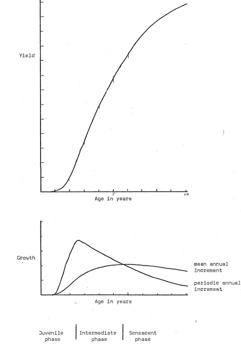
increases, a phase of relatively vigorous growth that changes into a senescent phase after mean annual increment culminates. These phases are shown diagramatically in Figure IV. 1.

Figure IV.1 also shows that there are two alternative ways of looking at such a model, the first as a yield model and the second as a growth model. If both growth and yield models are being developed simultaneously for use in practice then they should be compatible, compatibility being formally defined by Clutter (1963) as:

’’when the yield model can be obtained by summation of the predicted growth through the appropriate growth periods or, more precisely, when the algebraic form of the yield model can be derived by mathematical integration of the growth model.”

If the growth and yield models are not compatible according to this definition then two different model forms are being used.

COMPARISON OF GROWTH AND YIELD MODELS

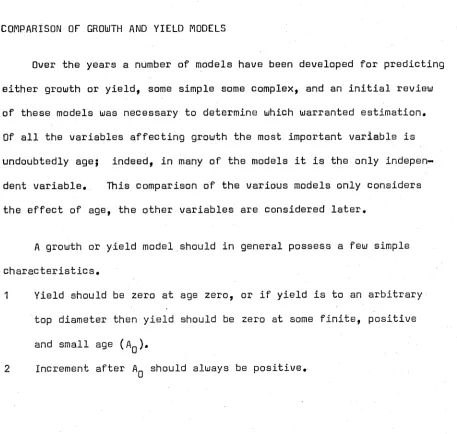
Over the years a number of models have been developed for predicting either growth or yield, some simple some complex, and an initial review of these models was necessary to determine which warranted estimation. Of all the variables affecting growth the most important variable is undoubtedly age; indeed, in many of the models it is the only indepen­ dent variable. This comparison of the various models only considers the effect of age, the other variables are considered later.

A growth or yield model should in general possess a few simple characteristics.

1 Yield should be zero at age zero, or if yield is to an arbitrary top diameter then yield should be zero at some finite, positive and small age ( A g ) .

43

Yield

Growth

Figure IV/. 1

Relationship between growth and yield

Age in years

mean annual increment

periodic annual

increment

Age in years

\

Juvenile

phase

Intermediate

phase

Senescent

3 Increment should have a single maximum (at age A^) and after this age It- should decrease q^> ii^c-rc.asc-s> ■

4 Yield should approach a maximum yield (Y x ) asymptotically.

Of course if the data are inadequate or if the model is to be used over a relatively restricted age range then even these requirements may be relaxed.

Table IV.1 summarises many of the models that have been developed in equation form, including both the growth (derivative) and yield (integral) equations to facilitate comparisons. For convenience and consistency some of the models have been reformulated slightly.

Graphical yield models

Graphical yield models have been used in the past in many countries, and in South Australia they have been used for many years to produce radiata pine yield tables. The techniques are flexible and easy to use, but do not allow an estimate to be made of precision, and they are clearly liable to bias..

The first radiata pine yield table in South Australia was produced by Gray in 1931 (Lewis, Keeves and Leech, 1975) using the limiting curve method attributed by Spurr (1952) to Baur in 1877. This method uses

single or spot estimates of yield to define upper and lower bounds to

yield, these being then divided anamorphicaily into site potential classes. As more data became available the yield table was revised by Solly in

1941 and later by Lewis in a series of revisions in 1953, 1957, 1960, 1963, 1968, 1970 and 1973 (Lewis, Keeves and Leech, 1976). As trend data became available the method changed to the directing curve trend method attributed by Spurr (1952) to Heyer in 184-5.