Analysing EEG brain signals using independent component analysis techniques

UNIVERSITY OF SOUTHERN QUEESLAND

ANALYSING EEG BRAIN SIGNALS USING

INDEPENDENT COMPONENT ANALYSIS TECHNIQUES

A dissertation submitted by

Janett G. St. H. Williams, MS, MA

For the award of Doctor of Philosophy

Dedication

To my mother Gretel Georgia Walters

a love for education drived her believe in me. Mom you died two years too soon

To my family

Abstract

The use of electroencephalography (EEG) in the medical field is evident in the effect it has on diagnosis and treatment of patients who suffer from some form of brain problem. These

signals however once collected are overlayed with artifacts. This thesis considers this problem

and seeks to solve using popular methods in the form of Independent Component Analysis (ICA)

and Wavelet Transform (WT).

Independent component analysis (ICA) is a popular blind source separation (BSS) technique that has proven to be promising for the analysis of EEG data. There are different estimators to developing these ICAs. Mutual Information is one of the most natural criteria when developing an estimator. Although utilized to some level it has always been difficult to calculate.

In this thesis I present a new algorithm which utilizes a contrast function related to Mutual

Information based on B-Spline functions. This thesis also investigates the creation of an algorithm which is based on a merger of Independent Component Analysis and Translation Invariant Wavelet Transform and goes on to merger the B-Spline ICA with the Translation

Invariant Wavelet Transform. In addition I apply Unscented Kalman Filtering as it does not

require any prior signal knowledge. Each algorithm will be examined and compared to ones in

literature tackling the same EEG problems; results will be drawn on the base of comparative tests

Certification of Dissertation

I certify that the ideas, experimental work, results, analyses, software and conclusions reported in this dissertation are entirely my own effort, except where otherwise acknowledged. I also certify that the work is original and has not been previously submitted for any other award, except where acknowledged.

November 24, 2011

Signature of Candidate Date

ENDORSEMENT

______________________________ _____________

Signature of Supervisor/s Date

Acknowledgement

Completing a Doctor of Philosophy in a very challenging subject is usually a long and

winding road; luckily I was not alone in this trip. The following were my travelling companions

in this journey and I would like to say a big thanks, as this work would not have been possible

without them.

Firstly I must thank God Almighty who completes things in the right season and who

declared that this is my season. I am sincerely thankful to my supervisor Dr. Yan Li, for having

believing in me and giving the necessary guidance and advice. In so doing she is responsible for

helping me develop into the scientist that I am becoming.

Thanks to the University of Technology, Jamaica for funding half of my tuition for the

time of my studies. Special thanks must be extended to the School of Computing and

Information Technology, especially Mr. Arnett B. Campbell, Head of School, who provided me

with the time and resources to conduct my research.

To my husband Marlon, my biggest supporter, reader and commenter, thank you for the

many nights you sacrificed your sleep.

To my pastor and friend, Rev. Dexter E. Johnson whose support was deeply appreciated

and who kept the church “at bay” while this thesis was being completed. I acknowledge my

students who in supporting and believing in me made working pleasurable and at time a

laughable experience.

Finally, thanks to my children – Melonie, MacAllister and Mahalia for their patience and

love in the long distance and my mother-in-law Jean Williams for her help in taking care of them

Table of Contents

Abstract ii

Acknowledgement iv

List of Figures ix

List of Tables xii

List of Algorithms xiii

List of Abbreviations xiv

List of Publications xvii

Chapter 1 – Introduction

1.1 Background 1

1.2 Justification for the Research 4

1.3 Methodology 5

1.4 Outline of Dissertation 11

1.5 Proposed Contributions of the Dissertation 12

1.6 Summary 13

Chapter 2 - Electroencephalograph

2.1 Introduction 14

2.2 Electroencephalograph Measuring System 17

2.3 Wave Analysis of the EEG 19

2.4 Uses of EEG 26

2.5 Artifacts in EEG 27

2.6 Denoising EEG 35

2.7 Methods 36

Chapter 3 – Denoising Methods

3.1 Independent Component Analysis 40

3.2 Wavelet Analysis 57

3.3 Filtering 66

3.4 Performance Measure for Methods 70

3.5 Summary 74

Chapter 4 – B-Spline Mutual Information ICA

4.1 The Mutual Information Estimator 75

4.2 B-Spline Function 80

4.3 Newly Designed ICA 84

4.4 Summary 98

Chapter 5 – Reliability of BMICA

5.1 Reasons for Reliability Testing for ICA Algorithms 99

5.2 Previous Research on Reliability 100

5.3 The ICASSO Reliability Test 101

5.4 Comparison ICA Algorithm Tested – FastICA 104

5.5 Results 105

5.6 Summary 120

Chapter 6 – MI Algorithms vs Non-MI Algorithms

6.1 Introduction 121

6.2 Experiment Setup 121

6.3 Results 122

6.4 Discussion 130

Chapter 7 – Unscented Kalman Filter

7.1 Introduction 132

7.2 EEG, EKF and UKF 132

7.3 Experiment 135

7.4 Results 136

7.5 Discussions 140

7.6 Summary 142

Chapter 8 – Improving Translation Invariant Wavelet Transform (TIWT)

8.1 Introduction 143

8.2 Translation Invariant Algorithm 143

8.3 Mergering Filters and WT 153

8.4 TIWT and BMICA Merger 166

8.5 Summary 179

Chapter 9 – Discussion and Conclusion

9.1 Summary 182

9.2 Links to Dissertation Goals 182

9.3 Conclusion 187

9.4 Actual Contribution of the Dissertation 188

9.5 Implications 189

9.6 Further Work 190

References 192

Appendix A 211

Appendix C 213

Appendix D 214

Appendix E 214

Appendix F 215

Appendix G 216

Appendix H 218

Appendix I 220

Appendix J 221

List of Figures

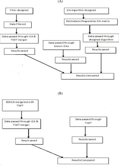
1.1 Work Flow of Dissertation 6

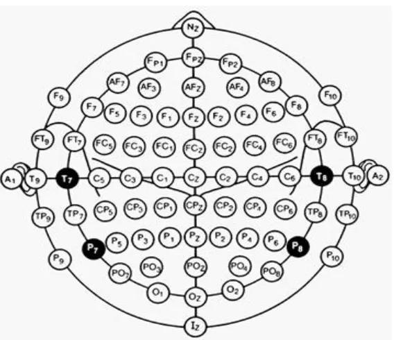
1.2 Distribution of Electrodes 8

1.3 Sample EEG Signals from a Male Subject 9

2.1 Structure of Typical Mammalian Neurons 14

2.2 Placement of EEG Electrodes on a Patient 15

2.3 Different Amplifiers Which Produce A Signal EEG Recording/Signal 16

2.4 A Simple Example of an Electroencephalography Machine 16

2.5 The International 10-20 System 18

2.6 Four of the Six Frequency Bands found in EEG Signals 19

2.7 One Second Recording of EEG Alpha Wave 20

2.8 A Schematic View of the Human Head Viewed From Above 20

2.9 One Second Recording of EEG Mu Wave 21

2.10 One Second Recording of EEG Beta Wave 22

2.11 One Second Recording of EEG Theta Wave 22

2.12 One Second Recording of EEG Delta Wave 23

2.13 One Second Recording of EEG Gamma Wave 23

2.14 Set of EEG signals Showing 3 of the Six Bands 24

2.15 EEG Activity is Dependent on the Level of Consciousness 25

2.16 One second Recording of clean pure EEG Signal 27

2.17 Eye Blink Artifact 28

2.18 Eye Movement Artifact 29

2.19 EOG Signal containing both Eye Blink and Eye movement artifacts 29

2.20 EEG Contaminated with EOG Producing Spikes 30

2.21 Ten Seconds Cardiac Movement Artifact 30

2.23 Muscle Activity Artifact - Chewing 31

2.24 Recording of a Glossokinetic Signal 32

2.25 One 60 Seconds Recording of a GSR Signal 33

2.26 Electrode Pop Artifact 34

2.27 Line Interference of 50Hz 34

3.1 Mathematical Model for ICA decomposition 43

3.2 Generalized ICA Algorithm 44

3.3 EEG Signals Being Broken Into ICs Using ICA 48

3.4 Difference between (A) Wave and (B) Wavelet 57

3.5 Several Different Families of Wavelets 59

3.6 Hard and Soft Thresholding Estimators Along With the Original Signal 63

3.7 Block Diagram of the Translation Invariant Wavelet Transform 63

3.8 Noisy EEG and its Wavelet Transform at Different Scales 66

4.1 Relationship between Mutual Information I(X:Y) and Entropies H(X) and H(Y) 76

4.2 Sample of Raw EEG Signal 87

4.3 EEG Signal After Denoised with BMICA algorithm 88

4.4 SIR Comparison (A) Fixed Point Algorithm (B) Non-fixed Point Algorithm 95

4.5 Amari Index (A) Fixed Point Algorithm (B) Non-fixed Point Algorithm 96

5.1 Sample of a Dendrogram 102

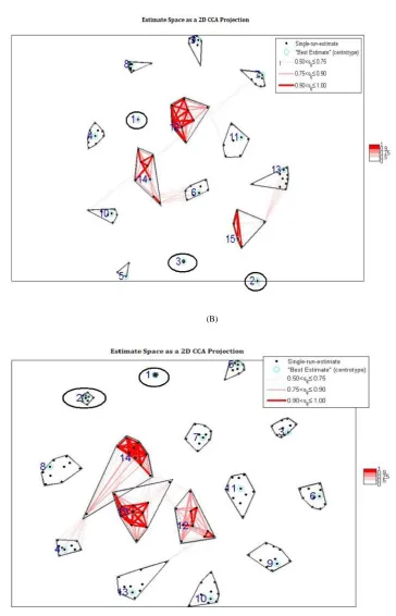
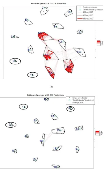
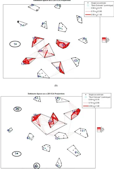
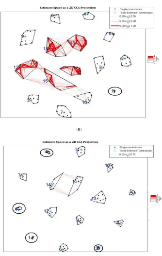
5.2 Cluster Plots for (A) BMICA (B) FastICA 106

5.3 Dendrogram for (A) BMICA (B) FastICA 108

5.4 Estimate Quality for (A) BMICA (B) FastICA 109

5.5 Estimates per cluster for (A) BMICA (B) FastICA 112

5.6 Centrotypes for (A) BMICA (B) FastICA 114

5.7 Cluster Plots for (A) FastICA(del-guas) (B) FastICA (sym-guas) 115

5.8 Cluster Plots for (A) FastICA(del-skew) (B) FastICA (sym-skew) 116

5.10 Cluster Plots for (A) FastICA(del-pow3) (B) FastICA (sym-pow3) 118

5.11 Cluster Plot for BMICA 119

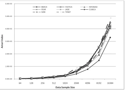
6.1 Amari Index for both Mutual Information and Non

Mutual Information Algorithms 124

7.1 First 14 Signals from Data Set Used 136

7.2 Channel 32 Showing First 150 Values With and Without Noise 137

7.3 True State of Signal and Estimates for (A) UKF (B) EKF 138

7.4 Estimation Errors and 3-σ Confidence Intervals for (A) UKF (B) EKF 139

7.5 Performance Comparison of the UKF and EKF filters. 141

8.1 EEG Signal Contaminated with EOG 145

8.2 Denoised EEG Signal for (A) TIWT (B) FastICA (C) RADICAL 146

8.3 SNR Comparison of EEG Signals 147

8.4 MSE Comparison of EEG Signals 148

8.5 PRD Comparison of EEG Signals 149

8.6 SIR Comparison with Six Other Algorithms 150

8.7 Amari Index Comparison with Five Other Algorithms 151

8.8 Proposed CTICA Artifacts Removal System 155

8.9 (A) EEG Signals with EOG (B) Denoised EEG Signals 157

8.10 Wave Coefficient (A) Before Denoising (B) After Denoising 158

8.11 SDR for 32 Real EEG Signals with EOG 162

8.12 Amari Results for the Four Algorithms 163

8.13 Raw EEG Signals 167

8.14 Denoised EEG using (A) WT (B) BMICW-WT 168

8.15 SIR Relations between BMICW-WT and TIWT 169

8.16 PSNR Relations between BMICW-WT and TIWT 171

8.17 Amari Index for BMICA-WT with Non-fixed Point Algorithms 173

8.19 SIR for BMICA-WT with Fixed Point Algorithms 175

List of Tables

4.1 MSE Comparison with (A) Fixed Point Algorithms (B) Non-Fixed Point Algorithms 89

4.2 PSNR Comparison with (A) Fixed Point Algorithms (B-C) Non-Fixed Point

Algorithms 90

4.3 SNR Comparison with (A) Non-Fixed Point Algorithms (B) Fixed Point Algorithms 92

4.4 SDR Comparison with (A) Fixed Point Algorithms (B) Non Fixed Point Algorithms 93

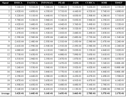
6.1 SDR for 20 EEG Signals 122

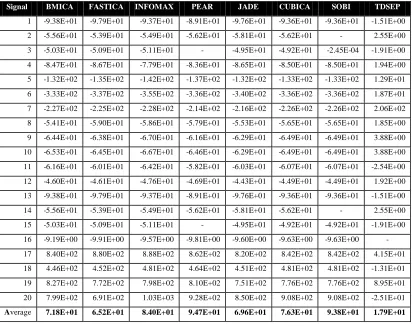
6.2 SIR for 20 EEG Signals 123

6.3 MSE for 20 EEG Signals 125

6.4 SNR for 20 EEG Signals 126

6.5 PSNR for 20 EEG Signals 127

7.1 MSE for 8 Channels 140

8.1 PSNR for 11 Real EEG Signals 152

8.2 MSE for 11 Real EEG Signals 152

8.3 MSE for 20 Real EEG with EOG Noise 159

8.4 MSE for 19 EEG with Artificial Added Noise 159

8.5 PSNR for 19 Real EEG with EOG noise 160

8.6 PSNR for 19 EEG with Artificial Added Noise 161

8.7 SDR for 19 EEG with Artificial Added Noise 161

8.8 SDR for 19 EEG Signal Sets 169

8.9 MSE for 18 EEG Signal Sets 172

8.10 MSE for (A) Fixed Point Algorithms (B) Non-fixed Point Algorithms 176

8.11 PSNR for (A) Fixed Point Algorithms (B) Non-fixed Point Algorithms 177

List of Algorithms

Algorithm 1 Algorithm for Uniform Cubic B-Spline Function 82

Algorithm 2 Algorithm to Generate B-Spline Estimated MI 84

Algorithm 3 Algorithm to Generate New ICA 86

Algorithm 4 Extended Kalman Filter 133

List of Abbreviations

α Level of Confidence

σ Standard Deviation

AL Average Link

ARMA Auto-Regressive Moving-Average

BMICA B-Spline Mutual Information Independent Component Analysis

BMICA-WT B-Spline Mutual Information Independent Component Analysis – Wavelet Transform

B-Spline Basis Spline

BSS Blind Source Separation

CCA Cuvilinear Component Analysis

CS Cycle Spinning

CT Computed Tomography

CTICA Cycle Spinning Wavelet Transform Independent Component Analysis

CubICA Cumulant-based Independent Component Analysis

CRB Cram´er-Rao lower bound

CWT Continuous Wavelet Transform

df Degree of Freedom

DSS Dynamic State Space

DWT Discrete Wavelet Transform

ECG/EKG Electrooculogram, -graphy

EEG Electroencephalogram, -graphy

EFICA Efficient FastICA

EKF Extended Kalman Filter

EMG Electromyogram, -graphy

EOG Electroculogram, -graphy

GSR Galvinic Skin Response

ICA Independent Component Analysis

IMA Infusion Motor Artifact

Infomax Information Maximization

JADE Joint Approximate Diagonalization Eignen Matrices

KDE Kernel Density Estimator

KF Kalman Filter

KL Kullback Leibler

KNN K Nearest Neighbour

Matlab Matrix Laboratory

MEG Magneto Encephalography

MI Mutual Information

MILCA Mutual Information Least-Dependent Component Analysis

ML Maximum Likelihood

MMI Minimum Mutual Information

MRI Magnetic Resonance Imaging

MSE Mean Square Error

p-value Probability Value

PCA Principal Component Analysis

PRD Percentage Root Mean Square Difference

PSNR Peak Signal to Noise Ratio

RADICAL Robust, Accurate, Direct Independent Component Analysis Algorithm

REM Rapid eye movement

SCCN Swartz Center for Computational Neuroscience

SDR Signal to Distortion Ratio

SIR Signal to Interference Ratio

SNR Signal to Noise Ratio

SOS Second Order Statistics

SWS Slow wave Sleep

SWT Stationary Wavelet Transform

TIWT Translation Invariant Wavelet Transform

TDSEP Temporal Decorrelation Source Separation

TVAR Time Varying Parameter Auto Regressive

UKF Unscented Kalman Filter

UNGM Univaiate Nonstationary Growth Model

UT Unscented Transformation

WF Weiner Filter

List of Publications

Journal Papers

Janett Walters-Williams and Yan Li, B-Spline Mutual Information Independent Component Analysis. In Journal of Computer Science and Network Security, Vol 10, No. 7, 2010 pp. 129-141.

Janett Walters-Williams and Yan Li, A New Approach to Denoising EEG Signals – Merger of Translation Invariant Wavelet and ICA. In International Journal of Biometric and Bioinformatics (IJBB), Volume 5, Issue 2, May 2011, pp 130 – 148

Janett Walters-Williams and Yan Li, Improving the Performance of Translation Wavelet Transform using BMICA. In International Journalof ComputerScience and Information Security (IJCSIS), Volume 9 No. 6 June 2011, pp 48-56

Janett Walters-Williams and Yan Li, Performance Comparison of Known ICA Algorithms to a Wavelet-ICA Merger. In Signal Processing: An International Journal (SPIJ), Volume 5, Issue 3. July 2011, pp 80-92

Janett Walters-Williams and Yan Li, Using Invariant Translation to Denoise EEG Signals, In American Journal of Applied Sciences, Volume 8, Issue 11, November 2011, pp 1122-1130

Janett Walters-Williams and Yan Li, Evaluation of an ICA-Filter-Wavelet Merger - A Case Study on Denoising EEG, In Press, International Journal of Computer Science Issues ("IJCSI"), Vol 8 Iss 4, July 2011

Janett Walters-Williams and Yan Li, BMICA-Independent Component Analysis Based On B-Spline Mutual Information Estimator, In Press, Signal & Image Processing: An International Journal (SIPIJ), September 2011

Janett Walters-Williams and Yan Li, BMICA-Independent Component Analysis based on B-Spline Mutual Information Estimation for EEG Signals, Submitted to Medical Engineering & Physics Journal, May 2011

Janett Walters-Williams and Yan Li, Reliability Testing of B-Spline Mutual Information Independent Component Analysis on EEG Signals, Submitted to to the International Journal of Systems Science, June 2011

Janett Walters-Williams and Yan Li, Denoising EEG: Making the Correct Choice of ICA Algorithm, Submitted to Clinical Neurophysiology, June 2011

Conference Papers

Janett Walters-Williams and Yan Li, Comparative Study of Distance Functions for Nearest Neighbours. In Proceedings of International Conference on Systems, Computing Sciences and Software Engineering (SCS2), December 5-13, 2008, Published in Advanced Techniques in Computing Sciences and Software Engineering, Vol. XIV, 2010, pp 79-84

Janett Walters-Williams and Yan Li, Estimation of Mutual Information: A Survey. In Proceedings of the Fourth International Conference on Rough Set and Knowledge Technology

(RSKT2009) July 14-16, 2009, Gold Coast, Australia, pp. 389-396

Janett Walters-Williams and Yan Li, Comparison of Extended and Unscented Kalman Filters applied to EEG Signals, In Proceedings of the 2010 IEEE/ICME International Conference on Complex Medical Engineering (CME2010) in Gold Coast, Australia, 13-15 July 2010, pp.

1

CHAPTER 1 - Introduction

1.1 Background

Biological processes are very complex mechanism, encompassing both neural and hormonal stimuli and responses, inputs and outputs in the most different forms, including physical material or information, and actions that could as well be mechanical, electrical or biochemical. Most of these processes are accompanied by or manifest themselves as signals that reflect their essential characteristics and qualities. Such signals are different in nature such as electrical and biochemical.

The development of diagnostic techniques based on these signal acquisition from the human body is commonly retained as one of the propelling factors of the advancements in medicine and biosciences. In fact, diseases or defects in biological systems almost always cause alterations in normal functions, giving birth to pathological processes that negatively impact on the performance and behavior of the systems themselves. If a good understanding of the system of interest is retained, in my case the neural network, it is possibly after the investigation of the signals and features originated by the system, to assess its state, discriminating between normal and abnormal responses. However, most physicians, like radiologists and neuroscientist, have to deal with additional problems when diagnosing the health state of the biological system from its signals. Like any acquisition systems, the instruments used for these biological systems are affected by non-idealities (artifacts) which by different degrees, negatively impact on the accuracy of these recordings. Accurate readings result once these artifacts have been removed.

2

human brain, and for medical diagnosis and treatment as well, especially for developing automated patient monitoring and computer-aided diagnosis. Extraction of relevant information on brain activity from measured electrical signals, called Electroencephalogram or EEG, (measures electrical potentials on the scalp surface that occur as a result of dynamic brain function [80]) is affected by various artifacts due to volume conduction through cerebrospinal fluid, skull, and scalp, as well as generated by experimental imperfections. These artifacts include: EOG (Eye-induced) artifacts (includes eye blinks and eye movements); ECG/EKG (cardiac) artifacts; EMG (muscle activation-induced) artifacts; and Glossokinetic artifacts. Developing and understanding advanced signal processing techniques for the analysis of EEG signals is crucial in the area of biomedical research. The presence of these artifacts may cause different interpretations by users of the EEG signals [146] which may result in misdiagnosis in the case of some patients. Artifacts must therefore be eliminated or attenuated.

Extraction of these artifacts is based on different data analysis techniques. These are loosely dichotomized into (i) hypothesis-driven methods, like the general linear model (GLM) [37], and (ii) data-driven model-free methods, such as principal component analysis (PCA) and Independent Component Analysis (ICA) [118]. The estimations of the problem of determining the brain electrical sources from potential patterns recorded on the scalp surface are mathematically undetermined [103] however, ICA algorithms have been proven to be a reasonably fit technique in removing these artifacts.

1.1.1 Research Problems, Hypothesis and Contributions

Although there have been many researchers and algorithms, after 60 years artifacts contaminations remain a problem [71]. Krishnaveni et al. [90] in their research found that of the six algorithms tested the Robust, Accurate, Direct Independent Component Analysis Algorithm (RADICAL) was considered to be the most robust ICA algorithms in the presence of artifacts in mixed data. Pandey et al.

3

RADICAL was the most robust, its performance was poor as all the algorithms assume the data to be homogeneous, which EEG is not, and operate based on the noise-free ICA model. Most if not all present algorithms therefore still do not remove all artifacts, resulting in degraded performances and interpretations that are still yet to be fully accurate.

Apart from the artifacts problem it has been found that most of the present algorithms perform best with certain data sizes e.g. Joint Approximate Diagonalization Eignen Matrices (JADE) which performs best on small signal set sizes [175]. There is presently none that can perform accurately given any data size therefore there is a problem of being adaptive.

Hyvarinen et al. [62] stated that the use of whitening in ICA helps to explain why the uses of Gaussian variables are forbidden. Most of the present ICA algorithms perform under the assumption that their data is non-gaussian; using ICA estimation can only be done up to an orthogonal transformation [61]. Separation can therefore fail when a Gaussian distribution is found within the data [120].

1.1.2 Dissertation Goals

This dissertation aims to present the design and implementation of robust ICA algorithms to separate Electroencephalography (EEG) signals from other signals described as artifacts. The new algorithms are expected to provide a more efficient way of removing these signals leaving EEG signals which can be interpreted by users. These algorithms will have the following features:

1. Robustness: The algorithms will be able to remove outliers from the signal data.

2. Accuracy: Removal of EOG and other underlying signals from the signal data.

4

4. Convergence: Able to have a fast convergence.

1.2 Justification for the Research

Based on literature investigations most EEG correction techniques focus on removing artifacts based on contamination by eye movements and blinks often called ocular (EOG) artifacts [24, 42, 71, 77]. There has been relatively little work done on other forms of artifacts such as cardiac signals, muscle activities and electrode noise. In 2007 the most widely spread method was to reject the EEG segments containing these artifacts thus removal, especially when there are limited data available and/or many artifacts present, may lead to an unacceptable loss of valuable data [1147].

The ICA techniques in existence are mainly based on the basic noise-free ICA definition in [61] where the artifacts term is usually omitted i.e.

x t( ) A s t( ) (1.1) where A is a 2x2 mixing matrix, s(t) the desired signal and x(t) is the observed signal in time (t). This is because this model seems to be sufficient for many applications and in many cases the number of the independent components (ICs) and observed mixtures may not be equal[62]. The algorithms based on this model produce results which are simpler and tractable [59]. These algorithms are perfect for artificial signal sets however real signals such as EEG always has some kind of artifacts present [62] resulting in Hyvärinen stating that canceling noise is a central yet an unsolved problem in EEG processing [59]. Literature therefore shows that the present algorithms either remove EEG data or allow for artifacts to remain after completion.

The level of performance for any ICA algorithms can be measured based on four areas:

5 2. The uniqueness of the components.

3. The robustness of the estimated dependencies against outliers and artifacts. 4. The robustness of the estimated components.

Literature on ICA algorithms shows that areas 2 and 4 have often be utilized and answered, however areas 1 and 3 have not been investigated much. ICA algorithms have the need to exploit an independence measure. Literature on Mutual Information (MI) has shown that it is an obvious candidate for measuring this independence [89, 159] and a good contrast function [20, 62] thus answering area 1. MI, however, is not extensively used for measuring interdependence because estimating it from statistical samples is not easy.

In the ICA literature very crude approximations to MI based on cumulant expansions are popular because of their ease of use [89] and have been very successful [20]. Hyvarinen [59] stated however that in their present use MI algorithms is far from optimal as far as robustness and asymptotic variance are concerned. These algorithms were also sensitive to artifacts. As they are now MI-based algorithms cannot answer neither areas 1 or 3 although designed to measure the independence of the components and considered a natural criterion to estimating ICA algorithms. To the best of my knowledge no researcher has implemented an algorithm which seeks to tackle all 4 areas. In 2004 the closest algorithm, Mutual Information Least-Dependent Component Analysis (MILCA), was created but it is slower than algorithms like FastICA and JADE [188].

1.3 Methodology

6 (A)

(B)

7

1.3.1 Algorithm Environment

The algorithms will be implemented within the following environments: (i) Laptop Environment 1 - This environment was based on Matrix Laboratory

(MATLAB) 7.8.0 (R2009) on a laptop with AMD Athlon 64x2 Dual-core Processor 1.80GHz.

(ii) Laptop Environment 2 - This environment was based on Matrix Laboratory (MATLAB) 7.10.0.499 (R2010) on a laptop with AMD Athlon 64x2 Dual-core Processor 1.80GHz

Both MATLAB environments contain the ICA and EEGLAB toolboxes which provide interactive graphic user interfaces allowing users to flexibly and interactively process their high-density EEG and other dynamic brain data using ICA. These toolboxes offer wealth of methods for visualizing and modeling event-related brain dynamics, both at the level of individual EEG datasets and/or across a collection of datasets brought together in an EEG studyset. The labs offer extensible, open-source platforms through which new algorithms can be shared with the world research community by contributing ‗plug-in' functions that appear automatically in the menus.

1.3.2 Datasets

There are two types of data that can be used in experiments – real data and synthetic data. In synthetic data the source signals are known as well as the mixing matrix A. In these cases the separation performance of the unmixing matrix W can be assessed using the known A and the quality of the unmixed signals yi can be

evaluated using the known source si. Biomedical signals however produce unknown

source signals. In this dissertation to test and evaluate my algorithms I utilize real EEG data, of different sizes, collected from the following sites:

1.3.2.1 Dataset 1

8

been recorded with a sampling rate of 128 Hz from 32 different locations on the scalp, resulting in 32 separate EEG signals. Below is a diagram showing the 32 locations on the scalp and the placement of the 32 measuring tools called electrodes (Figure 1.2).

Figure 1.2. Distribution of Electrodes (adapted from Practical Guide for Clinical Neurophysiologic Testing: EEG, Thoru Yamada, Elizabeth Meng, Lippincott Williams & Wilkins, 2009)

Each electrode contains 30,504 values. All data are real comprised of EEG signals from both human and animals. Data were of different types namely:

o Data set acquired is a collection of 32-channel data from one male subject who performed a visual task. Figure 1.3 shows 10 signals from this dataset as represented in Matlab.

9

were recorded at 2048 Hz sampling rate from 32 electrodes placed at the standard positions of the 10-20 international system.

o Data set is a collection of 32-channel data from 14 healthy subjects (7 males, 7 females, mean age 26 ranging from age 22 to 46) with normal or corrected to normal visison. They performed a go-nogo categorization task and a go-no recognition task on natural photographs presented very briefly (20 ms). Each subject responded to a total of 2500 trials. The data is CZ referenced, sampled at 1000 Hz usng the 10-20 international system. Data focuses on two groups of electrodes (i) frontal (Fz, FP1, FP2, F3,F4, F7,F8) and (ii) occipital (O1, O2, O1‘, O2‘ Oz, I, PO9, PO10, PO9‘, PO10‘ where the differential activity reached the highest amplitude.

10

1.3.2.2 Data Set 2

http://www.cs.tut.fi/~gomezher/projects/eeg/databases.htm. Data here contains

o Two EEG recordings (linked-mastoids reference) from a healthy 27-year-old male in which the subject was asked to intentionally generate artifacts in the EEG.

o Two 35 years-old males where the data was collected from 21 scalp electrodes placed according to the international 10-20 System with addition electrodes T1 and T2 on the temporal region. The sampling frequency was 250 Hz and an average reference montage was used. The electrocardiogram (ECG) for each patient was also simultaneously acquired and is available in channel 22 of each recording.

1.3.2.3 Data Set 3

http://www.meb.uni-bonn.de/epileptologie/science/physik/eegdata.html. Five data sets containing quasi-stationary, noise-free EEG signals. Each data set contains 100 single channel EEG segments of 23.6 sec duration recorded with a 128-channel amplifier system using an average common reference (omitting electrodes containing pathological activity). These segments, selected and cut out from continous multichannel EEG recordings, were obtained from (i) five healthy relaxed volunteers using a standardized electrode placement and (ii) five epileptic subjects in seizure activity. These signals were artificially contaminated.

1.3.2.4 Data Set 4

11

mental tasks. Data was provided in two ways: raw EEG signals and data with precomputed features.

1.3.2.5 Data Set 5

sites.google.com/site/projectbci. Data here is from a 21 age year old right-handed male with no medical conditions. EEG consists of actual random movement of left and right hand recordings with eyes closed. Each row represents one electrode. The order of electrode is FP1, FP2, F3, F4, C3, C4, P3, P4, 01, 02, F7, F8, T3, T4, T5, T6, F2, CZ, PZ. Recording was done at 500Hz using Neurofax EEG system.

1.4 Outline of Dissertation

This dissertation is focused on artifacts separation of real world EEG signals. In this attempt, my solutions are based on statistical methods called ICA and Wavelet Transformation (WT). In Chapter 2, I establish the basic background information on EEG needed for my analysis. Here I establish the need for separation techniques for the EEG signals. Subsequently, I analyze the techniques utilized in this research showing the relationship between them and the EEG signals in Chapter 3. In this chapter I focus on ICA, WT and Filtering as well as an overview of different ICA algorithms and performance measures utilized within the dissertation.

Chapter 4 focuses on the development of the B-Spline Mutual Information estimator and the resulting algorithm created B-Spline Mutual Information Independent Component Analysis (BMICA). Chapter 5 concentrates on discussing the reliability of BMICA while comparing it to known ICA algorithms.

12

Chapter 8 focuses on the effect of denoising using Translation Invariant Wavelet Transform (TIWT) and discusses merging TIWT with ICA and Unscented Kalman Filter (UKF) to create the algorithm named Cycle Spinning Wavelet Transform ICA (CTICA). In this chapter I also focus on improving TIWT with the merger of BMICA to produce BMICA-WT.

I conclude in Chapter 9 by outlining several of the issues that were introduced in this dissertation. Emphasis is given to the novel ideas presented throughout the text. In addition future areas of improvements and development are presented.

Several appendices have been included to present detailed information on the development of the algorithms created.

1.5 Proposed Contributions of the Dissertation

The scientific contributions of this dissertation should include the following.

o Experimental results are given using TIWT, UKF and an ICA method as a method of artifact reduction.

o The use of B-Spline Mutual Information estimator to create a new ICA algorithm.

o The merger of the new ICA and TIWT as a method of artifact reduction.

13

1.6 Summary

Since 1995 when the first algorithm, Infomax was introduced, ICA has been used to identify both temporally and functionally independent source signals in multi-channel EEG. It characteristically separates several important classes of non‐brain EEG artifact activity from the rest of the EEG signal into separate sources including eye blinks, eye movement potentials, electromyographic (EMG) and electrocardiographic (ECG) signals, line noise, and single‐channel noise. This important benefit of ICA makes it very important to the field of medicine. The removal of artifacts would present cleaner signals thus making it possible to detect with EEG the asymmetries connected to disorders in blood circulation, general disorders connected to poisoning as well as epileptic disorders.

14

CHAPTER 2- Electroencephalograph

2.1 Introduction

The human brain weighs approximately 3 lbs., and it is 3 lbs. of the most

complex software on earth. It is so sophisticated it makes the most ultra modern

super-computer look like an abacus in comparison. The brain is the boss of the body

and consists of about 100 billion cells. Most of these cells are called neurons which

are apart of the nervous system. Neurons communicate by sending an electrical

charge (potential) down the axon and across the synapse to the next neuron. Because

the neurons are not physically connected, chemical messengers called

neurotransmitters cross the synaptic gap to get the message to the next neuron [14].

These neurotransmitters then activate corresponding receptors in the post synaptic

neuron and generate post synaptic currents which then passes on to next synapse and

so on (Figure 2.1). Communication is therefore both electrical and chemical.

15

Doctors have learned that measuring this electrical activity can tell how the

brain is working and this activity is really a superposition of a large number of

electrical potentials arising from several sources (including brain cells i.e. neurons and artifacts) [148]. However, the potentials arising from independent neurons inside the brain, not their superposition, are of main interest to the physicians and researchers to describe the cerebral activity. Direct measurements from the different centers in the brain require placing electrodes inside the head, which needs surgery. This is not acceptable because it causes pain and risk for the subject [161].A better solution is to calculate the signals of interest obtained on the scalp as seen in Figure 2.2.

Figure 2.2: Placement of EEG electrodes on a patient, monitoring the different sectors of the brain for activities. (adapted from Hamlet on the Holodeck : the Future of Narrative in Cyberspace, Janett

Horowitz Murray, New York: Free Press, 1997)

These signals are the weighed sums of the neurons activity, the weights depending on the signal path from the brain cell to the electrodes. Because the same potential is recorded from more than one electrode, the signals from the electrodes are supposed to be highly correlated [161]. Researchers therefore collect recordings

16

Figure 2.3: Differential Amplifier which produces a signal EEG recording/signal (adapted from ebme.co.uk)

locations on the surface of the head. These potentials are simultaneously tested through individuals‘ amplifiers or channels. Recordings from anyone channel does not represent total discharge from a single underlying segment of the brain but represent the difference in potential between two (2) areas under each pair of electrodes (Figure 2.3) [16]. The machine used is called an electroencephalograph (Figure 2.4) and the recordings collected are called electroencephalogram (EEG) signals. From these recordings an accurate appraisal of departures from norms can be made.

Figure 2.4: A Simple Example of an Electroencephalograph Machine (adapted from

17 History

Studies about EEG began as early as 1870, but these studies had been carried out in animals. It was five years later that an English physician, Richard Caton discovered the presence of electrical current in the human brain. The information was recorded by the physician but no further research was done with it until Han

Berger. In 1924 Hans Berger, a German neurologist, took Caton‘s information and

put it to a test. He used his ordinary radio equipment to amplify the brain‘s electrical

activity so that he could observe the results on graph paper. Berger noticed that

rhythmic changes (brain waves) varied with the individual‘s state of consciousness and called the recorded signals Elektroenkephalogram [33]. This EEG represents complex irregular signals that may provide information about underlying neural activities in the brain.

2.2 Electroencephalograph Measuring System

There are different types of electroencephalographs; however the internationally standardized 10-20 system is the most widely used method to describe the location of scalp electrodes. It is based on the relationship between the location of an electrode and the underlying area of cerebral cortex and usually employs 21 electrodes. The positions are determined by dividing the skull into perimeters by connecting few reference points on human head.

Each perimeter has a letter (to identify the lobe) and a number or another letter to identify the hemisphere location. The letters used are: "F"-Frontal lobe, "T"-Temporal lobe, "C"-Central lobe, "P"-Parietal lobe, "O"-Occipital lobe. Even numbers (2,4,6,8) refer to the right hemisphere and odd numbers (1,3,5,7) refer to the left hemisphere. "Z" refers to an electrode placed on the midline; the smaller the number, the closer the position to the midline. Figure 2.5 shows the actual electrode placement on the head and from these points, the skull perimeters are measured in

18

the three main measurements: nasion (the delve at the top of the nose, level with the

eyes)–inion (bony lump at the base of the skull on the midline at the back of the head) preauricular points and circumference of the head.

Figure 2.5: The international 10-20 system seen from (A) left and (B) above the head. A = Ear lobe, C = central, Pg = nasopharyngeal, P = parietal, F = frontal, Fp = frontal polar, O = occipital. (C)

Location and nomenclature of the intermediate 10% electrodes, as standardized by the American Electroencephalographic Society. (adapted from Bioelectromagnetism Principles and Applications of Bioelectricand Biomagnetic Fields Jaakko Malmivuo, Robert Plonsey, Oxofrd University Press,

19

2.3 Wave Analysis of the EEG

In the brain the more neurons that work in synchrony, the larger the potential (amplitude) of the electrical oscillations measured in microvolts (mV) and the faster the neurons work together, the higher the frequency of the oscillations measured in Hertz (Hz). These two parameters: amplitude and frequency are the primary characteristics of brain waves. EEGs are the recordings of these tiny electrical potentials or waves which are generally less than 300µV [142].

Figure 2.6: Four of the Six Frequency Bands found in EEG Signals (adapted from Introduction to Biomedical Instrumentation Mandeep Singh, PHI Learning Private Ltd. 2010)

The waves basically have small amplitudes typically ranging from 1 µV to 100 µV in a normal adult and are approximately 10 mV to 20 mV when measured with subdural electrodes such as needle electrodes on the surface of the brain. The frequencies of these EEG waves, emitted from various regions of the brain, range from 0.5 Hz to100 Hz. This has presented a great deal of difficulty to researchers trying to interpret the large amount of data they receive from even one EEG

recording as depending on the frequency a recording can present six classical categories or bands for the EEG waves - delta, theta, alpha, beta, mu and gamma as described below. Figure 2.6 shows the frequency band for some of the waves.

2.3.1 Alpha (

α

) waves

These waves, seen in Figure 2.7, were the first to be discovered (around 1908

by Hans Berger) hence why they are called "Alpha waves". These

waves predominantly originate from the occipital lobe during wakeful relaxation

20

Figure 2.7: One second Recording of EEG Alpha Waves (adapted from Introduction to Biomedical Instrumentation Mandeep Singh, PHI Learning Private Ltd. 2010)

Alpha waves are not a measure of peace and serenity, nor are they indicative of an altered state of consciousness.They are indicative of lack of visual processing and

lack of focus: the less visual processing and the more unfocused, generally the

stronger the alpha waves. When a person closes his eyes and does not do any deep

thinking or concentrating on vivid imagery, alpha waves are usually quite strong.

Figure 2.8: A schematic view of the human head viewed from above with the nose at the top. When the eyes are open, the EEG signals show low-voltage random activity. When the eyes close (the time of the large signal in the electrode near the eyes) an alpha rhythm with a frequency of 11 cycles per

21

The waves generated here, called the occipital alpha waves, are the strongest EEG brain signals (Figure 2.8) usually being detected with the naked eye. Alpha waves generally are seen in all age groups but are most common in adults. Alpha activity disappears normally with attention (e.g., mental arithmetic, stress, opening eyes).

2.3.2 Mu (μ) waves

Mu waves (Figure 2.9) produce oscillations in the 8-13 Hz being located in the motor and sensorimotor cortex. It partly overlaps with other frequencies and reflects the synchronous firing of motor neurons in rest state. The amplitude of Mu varies when the subject performs movement consequently it is also known as the ―sensorimotor rhythm‖.

Figure 2.9: One Second Recording of EEG Mu Wave (adapted from, T. Trott, Electroencephalogram http://weirddreams.net/electroencephalogram-eeg/. 2009)

2.3.3 Beta (β) waves

Beta waves (Figure 2.10) are in the frequency range of human brain activity 12-30Hz with low voltage 5-30 μV and are usually split into three sections: High

Beta Waves (19Hz+); Beta Waves (15-18Hz); and Low Beta Waves (12-15Hz).

22

Figure 2.10: One second Recording of EEG Beta Wave (adapted from Introduction to Biomedical Instrumentation, Mandeep Singh, PHI Learning Private Ltd. 2010)

2.3.4 Theta (θ) waves

Theta Waves are the second slowest frequency of brain waves with

frequency in the 4–7 Hz range (Figure 2.11), regardless of their source. They are

associated with the early stages of sleep, the process of day-dreaming, drowsy, states of enhanced creativity, ―Super Learning,‖ deeper relaxation or meditation, and sleep-dream activity. These waves are of high amplitude and appear during states of arousals and powerful surges of emotion. In awake adults, these waves are abnormal if they occur in excess. Several types of brain pathology can give rise to abnormally strong or persistent cortical theta waves.

Figure 2.11: One second Recording of EEG Theta Wave (adapted from Introduction to Biomedical Instrumentation, Mandeep Singh, PHI Learning Private Ltd. 2010)

2.3.5 Delta (δ) waves

23

with the reticular formation and are responsible for the slowest form of mental processing.

Figure 2.12: One second Recording of EEG Delta Wave (adapted from Introduction to Biomedical Instrumentation, Mandeep Singh, PHI Learning Private Ltd. 2010)

Theta and delta waves are known collectively as slow waves.

2.3.6 Gamma (γ) waves

Gamma waves (Figure 2.13) have a frequency between 25 to 100 Hz, though 40 Hz is prototypical. They were initially ignored before the development of

digital electroencephalography as analog electroencephalography is restricted to

recording and measuring rhythms usually less than 25Hz. Gamma waves are thought to represent binding of different populations of neurons into a network for the purpose of carrying out certain cognitive or motor functions and have long been considered the brain‘s information and sensory-binding brainwave. They are usually

associated with perception, consciousness, higher mental and reasoning activities,

high levels of intelligence, compassion, high self-control, and feelings of natural happiness. They have also been linked to having a great memory and an increased perception of reality.

24

Although none of these waves is ever emitted alone as seen in Figure 2.14,

the state of consciousness of the individual may make one frequency more

pronounced than the others. For example an alert person displays a low amplitude EEG of mixed frequencies, while a relaxed person produces large amounts of sinusoidal waves, in the 8Hz to 13Hz frequency range, which are particularly prominent at the back of the head.

25

2.3.7 Flow of EEG Waves

The EEG signal is closely related to the level of consciousness of a person. As the activity increases, the EEG shifts to higher dominating frequency and lower amplitude. When the eyes are closed, the alpha waves begin to dominate the EEG. When the person falls asleep, the dominant EEG frequency decreases resulting in theta waves. In a certain phase of sleep, rapid eye movement called Rapid eye movement (REM) sleep occurs, the person dreams and has active movements of the eyes, which can be seen as a characteristic EEG signal. In deep sleep, the EEG has large and slow deflections called delta waves. No cerebral activity can be detected from a patient with complete cerebral death. Examples of the above-mentioned waveforms are given in Figure 2.15.

Figure 2.15: EEG activity is dependent on the level of consciousness. (adapted from Bioelectromagnetism Principles and Applications of Bioelectricand Biomagnetic Fields Jaakko

26

2.4 Uses of EEG

Understanding the brain is a huge part of Neuroscience, and the development of EEG was for the elucidation of such a phenomenon. The analysis of EEG waves has been the subject of several studies since EEG itself represents the brain activity for a subject and gives an objective mode of recording brain stimulation. In neurology EEG is used to:

Diagnose and Confirm Epilepsy

Distinguish and characterize seizures for treatment purposes such as epileptic, psychogenic non-epileptic, syncope (fainting), migraine and sub-cortical movement disorders

Localize the region of brain from which a seizure originates for work-up of possible seizure surgery

Check for problems with loss of consciousness or dementia.

Help find out a person's chance of recovery after a change in consciousness. Serve as an adjunct test for brain-death.

Study sleep disorders, such as narcolepsy.

Monitor the depth of general anesthesia and the amobarbital effect during the Wada test

Monitor for non-convulsive seizures/non-convulsive status epilepticus

Help find out if a person has a physical (in the brain, spinal cord, or nervous system) or mental health problem.

Detect diseases such as Creutzfeldt-Jakob diseases (CJD), Alzheimer‘s, and Schizophrenia.

Differentiate "organic" encephalopathy or delirium from primary psychiatric syndromes such as catatonia

27

EEG used to be a first-line method for the diagnosis of tumors, stroke and other focal brain disorders, but this use has decreased with the advent of anatomical imaging techniques such as Magnetic Resonance Imaging (MRI) and Computed Tomography (CT).

In cognitive neuroscience EEG is used to investigate the neural correlates of mental activities from low-level perceptual and motor processes to high-order cognition such as attention, memory, and reading. In cognitive psychology it is used to get a better understanding of how the brain influences the way a person thinks, feels and acts.

2.5 Artifacts in EEG

EEG is widely used by physicians and scientists to study brain function and to diagnose neurological disorders. Any misinterpretations can lead to misdiagnosis.

These signals must therefore present a true and clear picture about brain activities as seen in Figure 2.16. The poor spatial resolution of scalp EEG (limited to 1 centimeter) is due to the low conductivity of the skull, the cerebrospinal fluid and the meninges, which cause a reduction and dispersion of the activity originated in the cortex.

Figure 2.16: One second Recording of clean pure EEG Signal (adapted from Introduction to Biomedical Instrumentation, Mandeep Singh, PHI Learning Private Ltd. 2010)

Scalp EEG is also very sensitive to subject movement and external noise such as activation of the head, musculature, eye movements, interference from nearby electric devices, and changing conductivity in the electrodes due to the

28

All of these activities that are not directly related to the current cognitive processing

of the subject are collectively referred to as background activities. EEG signals are therefore highly attenuated and mixed with these non-cerebral impulses called

artifacts or noise which fall into two categories – physiologic and extra-physiologic

[95]. A true diagnosis can only be seen when all these noises are removed.

2.5.1 Physiologic Artifacts

Any source in the body which has an electrical dipole or generates an electrical or magnetic field is capable of producing physiologic artifacts. They are generated by some biological activities in the human body. Physiological signals have widely different sources. Below we discuss those which tend to overlay the EEG sigals

2.5.1.1 Electrooculogram (EOG)

Eye artifacts are often measured more directly in the electrooculargram (EOG), where pairs of electrodes are placed above and around the eyes. Unfortunately, these measurements are contaminants of the EEG signals of interest and so simple subtraction is not a removal option even if an exact model of EOG diffusion across the scalp is available [71]. In the frequency domain, ocular artifacts increase the power of EEG signals from 2Hz to 20 HzThese artifacts are of two types:

Figure 2.17: Eye Blink (adapted from L F Araghi, A New Method for Artifact Removing in EEG Signals, Proceedings of the International MultiConference of Engineers and Computer Scientists

29

Eye Blinking: The eye blink artifact (Figure 2.17) is very common in EEG data. It produces a high amplitude signal that can be many times greater than the EEG signals of interest. Because of its high amplitude an eye blink can corrupt data on all electrodes, even those at the back of the head.

Figure 2.18: Eye Movement(adapted from M. van de Velde, SignalValidation in Electroencephalography Research, PhD Thesis, Eindhoven University of Technology, 2000)

Eye Movement: Eye movement artifacts (Figure 2.18) are caused by the reorientation of the retinocorneal dipole [71, 125]. This artifact‘s diffusion across the scalp is stronger than that of the eye blink artifact.

Figure 2.19: EOG Signal containing both Eye Blink and Eye movement artifacts (adapted from JJM Kierkels, Validating and Improving the Correction of Ocular Artifacts in Electro encephalography,

Dissertation Abstracts International, 2007)

30

Figure 2.20: EEG contaminated with EOG producing spikes (adapted from P. Senthil Kumar, R. Arumuganathan, K. Sivakumar, C. Vimal, An Adaptive method to remove ocular artifacts from EEG

signals using Wavelet Transform Journal of Applied Sciences Research, 5(7): 741-745, 2009)

2.5.1.2 Cardiograph (ECG/ EKG)

Figure 2.21: Ten Seconds Cardiac Movement Artifact (adapted from Noise Removal from EEG Signals in Polisomnographic Records Applying Adaptive Filters in Cascade, M. Agustina Garcés

Correa, et al. Adaptive Filtering Applications, 2011)

31

Figure 2.22: EEG Signal corrupted with ECG/EKG (adapted from Artifact Removal from EEG Signals using Adaptive Filters In Cascade, A Garcés Correa et al, Journal of Physics: Conference

Series 90, 2007)

2.5.1.3 Electromyogram (EMG)

Muscle activity can be caused by activity in different muscle groups including the neck and facial muscles. Frontalis and temporalis muscles (e.g., clenching of jaw muscles) are common causes. Generally, the potentials generated in the muscles are of shorter duration than those generated in the brain (Figure 2.23) and are identified easily on the basis of duration, morphology, and rate of firing (i.e., frequency) [95]. Particular patterns of electromyogram (EMG) artifacts can occur in some movement disorders. Essential tremor and Parkinson disease can produce rhythmic 4-Hz to 6-Hz sinusoidal artifacts that may mimic cerebral activity.

32

2.5.1.4 Chewing and Sucking Movement – Glossokinetic

In addition to muscle activity, the tongue (like the eyeball) functions as a dipole, with the tip negative with respect to the base. In this case, the tip of the tongue is the most important part because it is more mobile. The artifact produced (Figure 2.24) by the tongue has a broad potential field that drops from frontal to occipital areas, although it is less steep than that produced by eye movement artifacts [95]. Chewing and sucking can produce similar artifacts. These are commonly observed in young patients, however, they also can be observed in patients with dementia or those who are uncooperative. Minor tongue movements can contaminate the EEG, especially in Parkinsonian and Tremor disorders.

Figure 2.24: Recording of a Glossokinetic Signal (adapted from Machine Learning Group, Department of Computer Science Pohang University of Science and Technology

http://mlg.postech.ac.kr/research/bci.html)

2.5.1.5 Galvinic Skin Response (GSR)

33

recordings occur as these changes produce Sodium Chloride (NaCl) and Lactic Acid (C3H6O3) from sweating which react with the metals of the electrodes resulting in huge slow baseline sways. Significant asymmetry also can be observed when a collection of sweat (e.g. subgaleal hematoma) is under or in the skin.

Figure 2.25: One 60 Seconds recording of a GSR Signal (adapted from Circuit Surgery http://www.circuitsurgery.co.za/)

2.5.2 Extra-physiologic Artifacts

Extra-physiologic artifacts include interference from electric equipment, kinesiologic artifacts caused by body or electrode movements, and mechanical artifacts caused by body movement.

2.5.2.1 The Electroencephalograph Machine

34

Figure 2.26: Example of Electrode Pop: a sudden sharp edge in the recorded signal, followed by an exponential decay, obscuring the EEG (adapted from M. van de Velde, SignalValidation in Electroencephalography Research, PhD Thesis, Eindhoven University of Technology, 2000)

2.5.2.2 Power Lines – Alternating Currents (50-60Hz)

Strong signals from Alternating Current (A/C) power supplies (Figure 2.27) can corrupt EEG data as it is transferred from the scalp electrodes to the recording device. The problem usually arises when the impedance of one of the active electrodes becomes significantly large between the electrodes and the ground of the amplifier. In this situation, the ground becomes an active electrode that, depending on its location, produces the 50-60-Hz artifact. This artifact is often filtered by notch filters, but for lower frequency line noise and harmonics this is often undesirable. If the line noise or harmonics occur in frequency bands of interest they interfere with EEG that occurs in the same band [74]. Notch filtering at these frequencies can remove useful information. Line noise can corrupt the data from some or all of the electrodes depending on the source of the problem.

Figure 2.27: Line Interference of 50Hz (adapted from Artifact Removal from EEG Recordings – An Overview, Rohtash Dhiman, et al., National Conference on Computational Instrumentation, CSIO

35

2.5.2.3 Infusion Motor Artifact (IMA)

An Intra Venous (IV) drip within a person can cause rhythmic, fast, low-voltage bursts, which may be confused for spikes. With the increasing use of automatic electric infusion pumps, a new type of artifact - IMA, has arisen. Morphologically, IMA appears as very brief spiky transients, sometimes followed by a slow component of the same polarity.

2.6 Denoising EEG Signals

Contamination of EEG data can occur at many points during the recording process. Most of the artifacts considered here are biologically generated by sources external to the brain [83]. Improving technology can decrease externally generated artifacts, such as line noise, but biological artifact signals must be removed after the recording process, thus denoising procedures must be introduced to remove these biological overlays from the EEG signals.

Denoising stands for the process of removing noise i.e. unwanted information, present in an unknown signal. Real EEG recordings are a combination of artifacts (noise) and the pure EEG signal. Mathematically it is defined as:

( ) ( ) ( )

E t S t N t (2.1)

36

Numerous methods have been proposed by researchers to achieve this denoising process in EEG and are even reviewed in [25, 77]. A brief write-up about the existing techniques for denoising EEG is described in the next section.

2.7 Methods

The removing of artifacts from an EEG recording can be categorized into two groups:

(i) Artifact rejection - removes the EEG signal which contains the artifact and (ii) Artifact correction - removes the artifacts from the EEG signal while

keeping the pure EEG signal.

The most popular methods for each category are described below.

2.7.1 Artifact Rejection

2.7.1.1 Basic Artifact Rejection

One common denoising strategy is to reject all EEG epochs containing artifacts larger than some arbitrarily selected EEG voltage level. This is artifact rejection. When limited data are available, or artifacts, such as EOG, occur too frequently the rejection of epochs contaminated with the artifacts usually results in a considerable loss of information and may be impractical for clinical data. Since EEG and some artifacts occupy the same frequency band, this method is ineffective [42].

2.7.1.2 Regression

37

then brain electrical activity can also contaminate the artifacts recordings. Therefore, subtracting a linear combination of the recorded artifacts from the EEG may not only remove artifacts but also interesting cerebral activity. Review of the technique is in [24-25].

2.7.1.3 Filtering

In order to reduce the cerebral activity, Lins et al. [100] suggested low-pass filtering of the artifacts. They recognized however that low-pass filtering removes all high frequency activity from the EOG signal, both of cerebral and ocular origins. The use of adaptive filtering, such as Bayesian [28, 170], prior to applying regression correction may substantially reduce problems from bidirectional contamination. Use of adaptive digital filters for artifacts removal, however requires a suitable reference model for training the filter.

2.7.2 Artifact correction

2.7.2.1 Principal Component Analysis (PCA)

PCA is a class of methods based on decomposing the EEG and artifacts into spatial components, identifying artifactual components and reconstructing the EEG without the artifactual components. Lagerlund et al. [94] used PCA to identify the artifactual components. Statistically, PCA decomposes the signals into uncorrelated, but not necessarily Independent Components (ICs) that are spatially orthogonal and thus it cannot deal with higher-order statistical dependencies. PCA also cannot completely separate artifacts from brain signals especially when they both have comparable amplitudes [94].

2.7.2.2 Independent Component Analysis (ICA)

38

neural activity from muscle and blink artifacts in spontaneous EEG data. Jung et al, [71] also showed using an extended version of the Infomax algorithm [8] that ICA can effectively detect, separate and remove activity in EEG records from a wide variety of artifactual sources. Vigon et al. [165] compared four methods of artifact removal and found that the two ICA methods, using Infomax and JADE were significantly better than PCA and simple EOG subtraction. The limitation of present ICA algorithms is that there is no guarantee that any particular algorithm can capture the individual source signals in its components [91].

2.7.2.3 Wavelet Transform

The newest form of denoising method is Wavelet Transform (WT). It has been used to study EEG signals [11, 111, 130, 134] successfully because of its good localization properties in time and frequency domain [40]. There have been many approaches to denoising using WT; those based on shrinkage are the most popular [110] where the EEG signals are decomposed into wavelets and noise removal done using thresholding and shrinkage. Akin [1] in his research compared WT with fast Fourier transform and found that WT was better in detecting brain diseases. His research was confirmed by Hermann et al [54]. Unser et al [163] showed that wavelet is good at denoising EEG signals as well as other biomedical signals. WT‘s capability in transforming a time domain signal into time and frequency localization helps to understand the behaviour of a signal better. WT however has limitations such as Gibbs phenomena [21].

2.8 Summary

39

40

Chapter 3 – Denoising Methods

Computer based methods for analysis and interpretation of biological signals have been the subject of intense research. It is obvious that automated systems for biological signal processing such as noise removal considerably improve or support the judgment of physicians that perform the signal analysis. The methods used to produce these helpful signals are therefore important. This chapter focuses on the three methods utilized within this research. It will also describe the performance measures ulitized as well as the different ICA algorithms.

3.1 Independent

Component Analysis

It is often said that we suffer from ―information overload‖ but we actually suffer from ―data overload‖. This is because we have access to a large amount of data containing relatively small amount of useful information [152]. We suffer this way in my daily lives as well as in the science disciplines. There is therefore the need to extract this useful information from data.

In the sciences a set of measured signals is essentially a mixture of underlying factors which are the driving forces to the signal set. Here ICA promises to reveal these forces which are underlying i.e. ICA will extract these factors called source signals which are buried within a measured signal [152].

3.1.1 ICA and Its History

3.1.1.1 What is ICA?

41

independent component signals or source signals [39]. The mixtures can be sound, electrical signals such as EEG or image such as fMRI. For ICA to work as defined there are some assumptions made:

1. Independence: Whereas electrical signals (s) are statistically independent their mixture is not i.e.

1 , 2 1 2

a b a b

s s s s for all a and b _(3.1)

This is because each source signal is shared between both mixtures such that the resultant commonality between signal mixtures ensures that they cannot be independent [152]. This mathematical definition of independence means that we can generate the additional information necessary to recover the original signals.

2. Complexity: The temporal complexity of any mixture is greater than or equals to its simplest complexity i.e. its least complexity constituted source signal. This ensures that extracting the least complex signal from a set of signal mixtures yield a source signal [152].

Based on the assumption that if different signals are from different sources then those signals are statistically independent ICA works on the implication of the reversal of this assumption resulting in assumption 3: