High-order upwind methods based on C2-continuous two-node integrated-RBF elements for viscous flows

two-node integrated-RBF elements for viscous flows

D.-A. An-Vo1, N. Mai-Duy1and T. Tran-Cong1

Abstract: In this paper, 2-node integrated radial basis function elements (IRBFEs) [CMES, vol.72, no.4, pp.299-334, 2011] are further developed for the simulation of incompressible viscous flows in two dimensions. Emphasis is placed on (i) the incorporation of C2-continuous 2-node IRBFEs into the subregion and point col-location frameworks for the discretisation of the stream function-vorticity formu-lation on Cartesian grids; and (ii) the development of high order upwind schemes based on 2-node IRBFEs for the case of convection-dominant flows. High levels of accuracy and efficiency of the present methods are demonstrated by solutions of several benchmark problems defined on rectangular and non-rectangular domains.

Keywords: integrated-radial-basis-function elements, Cartesian grid, control vol-ume, subregion collocation, point collocation, local approximation, upwind scheme.

1 Introduction

Cartesian-grid-based subregion/point collocation methods can be very economical owing to the facts that (i) generating a grid and integrating the governing equations in these methods are low-cost; and (ii) FFT can be applied to accelerate computa-tional processes, e.g. Huang and Greengard (2000). The approximations for the dependent variables and their spatial derivatives can be constructed globally on the whole grid or locally on small segments of the grid. Examples of local approxima-tion schemes include standard control-volume (CV) methods and finite-difference methods. For the former, the fluxes are estimated by a linear variation between two grid points, e.g. Patankar (1980); Huilgol and Phan-Thien (1997). The use of two grid points allows for the consistency of the fluxes at CV faces - one of the four ba-sic rules to guarantee a phyba-sically realistic solution (Patankar (1980)). For the latter, local approximations can be constructed in each direction independently using two nodes (first-order accuracy) and three nodes (second-order accuracy). With two-1_{Computational Engineering and Science Research Centre, Faculty of Engineering and Surveying,}

node-based local approximations, Cartesian grid based methods typically produce solutions which are continuous for the fields but not for their partial derivatives, i.e.

C0 continuity. The grid thus needs to be sufficiently fine to mitigate the effects of discontinuity of partial derivatives.

The Navier-Stokes (N-S) equations involve two main terms, namely convection and diffusion. At high values of the Reynold number, the convection term is dominant and the numerical simulation of the N-S equations becomes challenging. Various treatments for the convection term have been proposed in the literature. Those which take the influence of the upstream information of the flow into account, e.g. the upwind differencing (Courant, Isaccson, and Rees (1952); Gentry, Martin, and Daly (1966)), hybrid (Spalding (1972)), power-law (Patankar (1981)) and QUICK (Leonard (1979)) schemes are known to provide a very stable solution. To maintain a high level of accuracy, an effective way is to employ high-order upwind schemes with the deferred-correction strategy, e.g. Khosla and Rubin (1974); Ghia, Ghia, and Shin (1982).

Radial basis functions (RBFs) have been successfully used for the approximation of scattered data. They have recently emerged as an attractive tool for the solution of ordinary and partial differential equations (ODEs and PDEs), e.g. Fasshauer (2007); Atluri and Shen (2002); Chen, Karageorghis, and Smyrlis (2008). RBF-based approximants are able to produce fast convergence especially for regular node arrangements such as those based on Cartesian grids. They can be con-structed through a conventional differentiation process, e.g. Kansa (1990), or an integration process, e.g. Mai-Duy and Tran-Cong (2001); Mai-Duy and Tanner (2005); Mai-Duy and Tran-Cong (2005). The latter helps avoid the reduction of convergence rate caused by differentiation and provide effective ways of impos-ing the derivative boundary values. RBF-based approximants can be constructed globally or locally. Global RBF-based methods are very accurate, e.g. Cheng, Golberg, Kansa, and Zammito (2003); Huang, Lee, and Cheng (2007). However, they result in a system matrix that is dense and usually highly ill-conditioned. The use of RBF-approximants in local forms has the ability to circumvent these dif-ficulties, e.g. Shu, Ding, and Yeo (2003); Šarler and Vertnik (2006); Divo and Kassab (2007). Recently, a local high order approximant based on 2-node elements and integrated RBFs (IRBFs) for solving second-order elliptic problems in the CV framework has been proposed by An-Vo, Mai-Duy, and Tran-Cong (2011). In such 2-node elements (IRBFEs), the integration constants are exploited to include the first derivatives at the element extremes in the approximations. It was shown that such elements lead to a C2-continuous solution rather than the usual C0-continuous solution.

point collocation frameworks for solving the N-S equations in the stream function-vorticity formulation on Cartesian grids. Unlike conventional finite-element-based methods, the proposed methods can guarantee inter-element continuity of deriva-tives of the stream function and vorticity of orders up to 2. At high values of the Reynolds number, to achieve both good accuracy and stability properties, several high-order upwind schemes are proposed. The resultant system of algebraic equa-tions is sparse and banded; the solution accuracy can be controlled by means of the number of RBFs and/or the shape parameter. Several viscous flows defined on rectangular and non-rectangular domains are considered to verify the proposed methods.

The remainder of the paper is organised as follows. Brief reviews of the governing equations and integrated RBF elements are given in Section 2 and 3, respectively. Section 4 describes the proposed C2-continuous subregion/point collocation tech-niques for the stream function-vorticity formulation. In Section 5, two benchmark problems, namely the lid-driven cavity flow and the flow past a circular cylinder in a channel, are presented to demonstrate the attractiveness of the present techniques. Section 6 concludes the paper.

2 Governing equations

The dimensionless N-S equations for steady incompressible planar viscous flows, subject to negligible body forces, can be expressed in terms of the stream function

ψ and the vorticityωas follows

∂2_ψ

∂x2 +

∂2_ψ

∂y2 +ω=0, (1)

∂2ω

∂x2 +

∂2ω

∂y2 =Re

_∂ψ

∂y

∂ω ∂x −

∂ψ ∂x

∂ω ∂y

, (x,y)T∈Ω, (2)

where Re=U L/νis the Reynolds number, in which L is the characteristic length,

U the characteristic speed of the flow andν the kinematic viscosity. The vorticity

and stream function variables are defined by

ω=∂v ∂x−

∂u

∂y, (3)

∂ψ ∂y =u,

∂ψ

∂x =−v, (4)

Pozrikidis (1997)) is applied to obtain the structure of a steady flow. The governing equations (1) and (2) are modified as

∂2_ψ

∂x2 +

∂2_ψ

∂y2 +ω=

∂ψ

∂t , (5)

∂2ω

∂x2 +

∂2ω

∂y2 −Re _∂ψ

∂y

∂ω ∂x −

∂ψ ∂x ∂ω ∂y =∂ω

∂t . (6)

Solutions to (5) and (6), which are obtained from integrating the equations from a given initial condition up to the steady state, are also solutions to (1) and (2) respectively.

In the case of subregion collocation, one needs to define control volumes for grid nodes. Integrating (5) and (6) over a CV of a grid point P,ΩP, leads to the following

equations

Z

ΩP _∂2ψ

∂x2 +

∂2ψ

∂y2

dΩP+

Z

ΩP

ωdΩP=

Z

ΩP

∂ψ

∂t dΩP, (7)

Z

ΩP _∂2_ω

∂x2 +

∂2_ω

∂y2

dΩP−

Z ΩP Re _∂ψ ∂y ∂ω ∂x −

∂ψ ∂x

∂ω ∂y

dΩP=

Z

ΩP

∂ω

∂t dΩP, (8)

which ensure that the flow field is conservative for a finite CV. Applying the Green theorem to (7) and (8), one has

I

ΓP

_∂ψ

∂xdy−

∂ψ ∂ydx

+

Z

ΩP

ωdΩP=

Z

ΩP

∂ψ

∂t dΩP, (9)

I

ΓP

_∂ω

∂x −Reω

∂ψ ∂y

dy−

_∂ω

∂y +Reω

∂ψ ∂x dx = Z ΩP ∂ω

∂t dΩP, (10)

whereΓPis the CV boundary. The governing differential equations (5) and (6) are

thus transformed into a CV form (7)-(8) or (9)-(10). It is noted that no approxima-tion is made at this stage.

3 Definition of integrated-RBF elements

3.1 Brief review of integrated RBFs

function are given by

∂2φ

∂η2(x) =

n

∑

i=1

wi

q

(x−ci)2+a2i = n

∑

i=1

wiIi(2)(x), x∈Ω, (11)

∂φ ∂η(x) =

n

∑

i=1

wiIi(1)(x) +C1(θ), (12)

φ(x) = n

∑

i=1

wiIi(0)(x) +C1(θ)η+C2(θ), (13)

whereΩis the domain of interest,φ a function, (η,θ) the two components of x,

n the number of RBFs,{wi}ni=1 the set of RBF weights, C1(θ)and C2(θ)the

con-stants of integration which are functions ofθ, I_i(2)(x)conveniently denotes the MQ whose centre and shape parameter are, respectively, ciand ai, Ii(1)(x) =

R

I_i(2)(x)dη, and I_i(0)(x) =RI_i(1)(x)dη. Explicit forms of I_i(1)(x) and I_i(0)(x) can be found in Mai-Duy and Tran-Cong (2001). In Mai-Duy and Tran-Cong (2003), the shape pa-rameter was simply chosen as ai=βhi in whichβ is a given positive number and

hithe distance between ciand its nearest neighbour.

When the analysis domainΩis a line segment, e.g. in the Cartesian direction η, expressions (11), (12) and (13) reduce to

∂2_φ

∂η2(η) = d2φ dη2 =

n

∑

i=1

wi

q

(η−ci)2+a2i = n

∑

i=1

wiIi(2)(η), (14)

∂φ ∂η(η) =

dφ dη =

n

∑

i=1

wiIi(1)(η) +C1, (15)

φ(η) =

∑

wiI_i(0)(η) +C1η+C2, (16)

where C1and C2are simply constant values.

Expressions (14), (15) and (16), called 1D-IRBFs, can also be used in conjunc-tion with Cartesian grids for solving 2D problems. Advantages of 1D-IRBFs over 2D-IRBFs ((11)-(13)) are that they possess some “local” properties and are con-structed with a much lower cost. However, numerical experiments show that 1D-IRBFs still cannot work with large values ofβ. In An-Vo, Mai-Duy, and Tran-Cong (2011), 1D-IRBF-based schemes were further localised to 2-node IRBF elements (IRBFEs).

3.1.1 Two-node IRBFEs

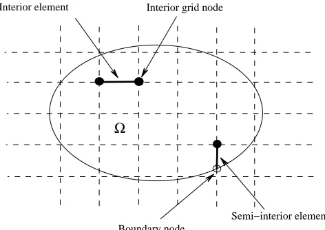
the case of non-rectangular domain, grid points outside the problem domain are re-moved while grid points inside the problem domain are taken to be interior nodes. Boundary nodes are defined as the intersection of the grid lines and the bound-aries. Over straight-line segments between two adjacent nodal points, 1D-IRBFs are utilised to represent the variation of the field variable and its derivatives, which are called 2-node IRBFEs. It can be seen that there are two types of elements, namely interior and semi-interior elements. An interior element is formed using two adjacent interior nodes while a semi-interior element is generated by an inte-rior node and a boundary node (Fig. 1).

3.1.2 Interior elements

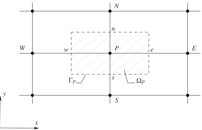
1D-IRBF expressions for interior elements are of similar forms. Consider an inte-rior element,η∈[η1,η2], and its two nodes are locally named as 1 and 2. Letφ(η) be a function andφ1,∂φ1/∂η,φ2and∂φ2/∂ηbe the values ofφand∂φ/∂ηat the two nodes, respectively (Fig. 2). The 2-node IRBFE scheme approximates φ(η)

using two MQs whose centres are located atη1andη2. Expressions (14), (15) and (16) become

∂2_φ

∂η2(η) =w1 q

(η−c1)2+a21+w2 q

(η−c2)2+a22=w1I1(2)(η) +w2I2(2)(η),

(17)

∂φ

∂η(η) =w1I₁(1)(η) +w2I₂(1)(η) +C1, (18)

φ(η) =w1I₁(0)(η) +w2I₂(0)(η) +C1η+C2, (19)

where I_i(1)(η) =RI_i(2)(η)dη, I_i(0)(η) =RI_i(1)(η)dη with i= (1,2), and C1and C2 are the constants of integration. By collocating (19) and (18) at η1 and η2, the relation between the physical space and the RBF coefficient space is obtained      φ1 φ2 ∂φ1 ∂η ∂φ2 ∂η     

| {z }

b φ =     

I₁(0)(η1) I₂(0)(η1) η1 1

I₁(0)(η2) I2(0)(η2) η2 1

I₁(1)(η1) I2(1)(η1) 1 0

I₁(1)(η2) I₂(1)(η2) 1 0     

| {z }

I     w1 w2 C1 C2    

| {z }

b

w

, (20)

whereφbis the nodal-value vector,I _{the conversion matrix, andw the coefficientb}

owing to the presence of integration constants. Solving (20) yields

b

w=I−1φb_{. (21)}

Substitution of (21) into (19), (18) and (17) leads to

φ(η) =hI₁(0)(η),I₂(0)(η),η,1iI−1φb_{, (22)} ∂φ

∂η(η) =

h

I₁(1)(η),I₂(1)(η),1,0iI−1φb_{, (23)}

∂2φ

∂η2(η) = h

I₁(2)(η),I₂(2)(η),0,0iI−1φb_{. (24)}

They can be rewritten in the form

φ(η) =ϕ1(η)φ1+ϕ2(η)φ2+ϕ3(η)∂φ_∂η1+ϕ4(η)∂φ_∂η2, (25)

∂φ ∂η(η) =

dϕ1(η) dη φ1+

dϕ2(η) dη φ2+

dϕ3(η) dη

∂φ1

∂η +

dϕ4(η) dη

∂φ2

∂η, (26)

∂2φ

∂η2(η) =

d2ϕ1(η) dη2 φ1+

d2ϕ2(η) dη2 φ2+

d2ϕ3(η) dη2

∂φ1

∂η +

d2ϕ4(η) dη2

∂φ2

∂η, (27)

where{ϕi(η)}4_i=1is the set of basis functions in the physical space. These

expres-sions allow one to compute the values ofφ,∂φ/∂η, and∂2φ/∂η2 _{at any pointη} in[η1,η2]in terms of four nodal unknowns, i.e. the values of the field variable and its first-order derivatives at the two extremes (also grid points) of the element.

3.1.3 Semi-interior elements

As mentioned earlier, a semi-interior element is defined by two nodes: an interior node and a boundary node. The subscripts 1 and 2 are now replaced with b (b represents a boundary node) and g (g an interior grid node), respectively. Assume that the value ofφis given atηb. The conversion system can be formed as

   φb φg ∂φg ∂η   =   

I_b(0)(ηb) Ig(0)(ηb) ηb 1

I_b(0)(ηg) Ig(0)(ηg) ηg 1

I_b(1)(ηg) Ig(1)(ηg) 1 0

       wb wg C1 C2   

It leads to

φ(η) =ϕ1(η)φb+ϕ2(η)φg+ϕ3(η)∂φ_∂ηg, (29)

∂φ ∂η(η) =

dϕ1(η) dη φb+

dϕ2(η) dη φg+

dϕ3(η) dη

∂φg

∂η , (30)

∂2φ

∂η2(η) =

d2ϕ1(η) dη2 φb+

d2ϕ2(η) dη2 φg+

d2ϕ3(η) dη2

∂φg

∂η . (31)

It can be seen that the conversion matrix in (28) is under-determined and its in-verse can be obtained using the SVD technique (pseudo-inversion). Owing to the facts that point collocation is used and the RBF conversion matrix is not over-determined, the boundary conditionφb is imposed in an exact manner. For other

types of semi-interior elements, the reader is referred to An-Vo, Mai-Duy, and Tran-Cong (2011) for details.

4 Proposed C2-continuous subregion/point collocation methods

In this study, 2-node IRBFEs are extended to the solution of the stream function-vorticity formulation. In addition, several high-order upwind schemes are incor-porated into the 2-node IRBFE methods to enhance their performance for the case of convection-dominant flows. The proposed methods lead to a sparse system and their solution is a C2function across IRBFEs.

4.1 Discretisation of governing equations

Two formulations, namely subregion collocation and point collocation, are em-ployed to discretise the governing differential equations. As mentioned earlier, the structure of a steady flow is found through the method of false transients. Time derivative terms in (5) and (6) are simply approximated here with a first-order back-ward difference.

4.1.1 Subregion collocation

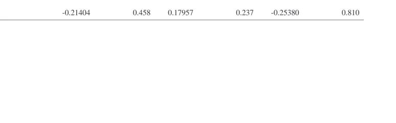
Consider a grid point P surrounded by a rectangular control volumeΩP (Fig. 3).

There are no gaps and overlapping regions between control volumes. For integrals involving the rate of change and generation, the value of the quantity at P is as-sumed to prevail overΩP. Using the middle-point rule to evaluate the integrals of

the convection and diffusion terms overΩP, equations (9) and (10) become

−AP

∆tψP+

_∂ψ

∂x

e ∆y−

_∂ψ

∂x

w ∆y+

_∂ψ

∂y

n ∆x−

_∂ψ ∂y s ∆x

=−AP

(32)

−AP

∆tωP+

_∂ω

∂x

e ∆y−

_∂ω

∂x

w ∆y+

_∂ω

∂y

n ∆x−

_∂ω ∂y s ∆x +Re −

ω∂ψ_∂

y

e ∆y+

ω∂ψ_∂

y

w ∆y+

ω∂ψ_∂

x

n ∆x−

ω∂ψ_∂

x

s ∆x

=−AP

∆tω

0

P,

(33) where the superscript 0 represents the value obtained from the previous time level; the subscripts e,w,n and s denote the values of the property at the intersections of

grid lines and the east, west, north and south faces of a CV; and AP the volume

ofΩP. It can be seen that equations (32) and (33) require the estimation of first

derivative values ofψ andωat the interface points e,w,n and s.

4.1.2 Point collocation

Consider a grid point P. Collocating (5) and (6) at P, one obtains

−ψP

∆t +

∂2ψ

P ∂x2 +

∂2ψ

P ∂y2 =−

ω0 P+ ψ0 P ∆t , (34)

−ω_∆P

t +

∂2ω

P ∂x2 +

∂2ω

P ∂y2 −Re

_∂ψ

P ∂y

∂ωP ∂x −

∂ψP ∂x

∂ωP ∂y

=−ω 0

P

∆t. (35)

It can be seen that equations (34) and (35) require the estimation of both first and second derivative values ofψandω at the collocation point P.

4.2 Approximations of diffusion term

The diffusion term is treated implicitly. Its role is important at regions where the strength of the convection term is small. 2-node IRBFEs are employed here for the approximation of the second terms on the LHSs of (32) and (33) in the subregion collocation framework and (34) and (35) in the point collocation framework. Let

E,W,N and S denote the east, west, north and south neighbouring nodes of P,

respectively. One can form 4 two-node IRBFEs, namely W P,PE,SP and PN.

4.2.1 Subregion collocation

In the case that W P and PE are interior elements, the values of the flux at x=xe

and x=xware computed by using (26)

_∂φ

∂x

e

= dϕ1(xe)

dx φP+

dϕ2(xe)

dx φE+

dϕ3(xe)

dx

∂φP ∂x +

dϕ4(xe)

dx

∂φE

∂x , (36)

_∂φ

∂x

w

= dϕ1(xw)

dx φW+

dϕ2(xw)

dx φP+

dϕ3(xw)

dx

∂φW ∂x +

dϕ4(xw)

dx

∂φP

whereφ representsψ andω.

In the case that W P is a semi-interior element, the value of the flux at x=xw is

computed by using (30) _∂φ

∂x

w

= dϕ1(xw)

dx φW+

dϕ2(xw)

dx φP+

dϕ3(xw)

dx

∂φP

∂x . (38)

Expressions for the flux at y=ynand y=ysare of similar forms.

4.2.2 Point collocation

The values of∂2ψ/∂x2and∂2ω/∂x2at P can be derived from 2-node IRBFEs in the x direction, i.e. W P and PE. It will be shown later that these two elements give the same results, and one can thus choose one of them for calculation, e.g.

W P. Through (27) if W P is an interior element and (31) if W P is a semi-interior

element, the required values are, respectively, estimated as

∂2φ

P ∂x2 =

d2ϕ1(xP)

dx2 φW+

d2ϕ2(xP)

dx2 φP+

d2ϕ3(xP)

dx2

∂φW ∂x +

d2ϕ4(xP)

dx2

∂φP

∂x (39)

and

∂2φ

P ∂x2 =

d2ϕ1(xP)

dx2 φW+

d2ϕ2(xP)

dx2 φP+

d2ϕ3(xP)

dx2

∂φP

∂x , (40)

whereφ representsψ andω.

The values of∂2ψ/∂y2and∂2ω/∂y2at P can be computed in a similar fashion.

4.3 Approximations of convection term

At high values of the Re number, the third term (i.e. convection term) on the LHS of (33) or (35) is dominant and strongly affects the stability of a numerical solution. From a physical point of view, convection is directed by the velocity field from the upstream to the downstream of the flow. Three high-order upwind schemes, namely Scheme 1, Scheme 2 and Scheme 3, are proposed here for the discretisation of the convection term.

4.3.1 Scheme 1 for subregion collocation

This scheme is concerned with an upwind treatment with the deferred correction strategy. Let f be the intersection of the CV face and the grid line. The value ofω at point f is computed as

whereωUis the upstream value and∆ωf the correction term that is a known value.

It is noted that f represents w,e,s and n. ∆ωf is presently derived from the 2-node

IRBFE approximation, i.e. (25) and (29). As an example, when f ≡w and uw>0,

one has

ωU=ωW, (42)

∆ωf = (ϕ1(xw)−1)ωW0 +ϕ2(xw)ωP0+ϕ3(xw)∂ω

0

W

∂x +ϕ4(xw)

∂ω0

P

∂x , (43)

where the superscript 0 is used to denote the values obtained from the previous time level. For a special case, where W is a boundary point, expression (43) reduces to

∆ωf = (ϕ1(xw)−1)ωW0 +ϕ2(xw)ωP0+ϕ3(xw)∂ω

0

P

∂x . (44)

When the solution reaches a steady state, ωfs are purely predicted by 2-node

IRBFEs and their accuracy is thus recovered. Velocity values in the convection term are simply estimated by a linear profile

_∂ψ ∂y e =1 2 _∂ψ0 P ∂y +

∂ψ0 E ∂y , (45) _∂ψ ∂y w =1 2 _∂ψ0 W ∂y +

∂ψ0 P ∂y , (46) _∂ψ ∂x n =1 2 _∂ψ0 P ∂x +

∂ψ0 N ∂x , (47) _∂ψ ∂x s =1 2 _∂ψ0 S ∂x +

∂ψ0

P ∂x

. (48)

4.3.2 Scheme 2 for point collocation

Without loss of generality, assuming that uP >0. W thus becomes an upstream

node. A special approximation is constructed over W P for the purpose of

comput-ing∂ωP/∂x; not onlyωW and ∂ωW/∂x but also∂2ωW/∂x2 are employed in the

conversion process      ωP ωW ∂ωW ∂η ∂2_ω W ∂η2     =     

I₁(0)(xP) I2(0)(xP) xP 1

I₁(0)(xW) I2(0)(xW) xW 1

I₁(1)(xW) I₂(1)(xW) 1 0

I₁(2)(xW) I2(2)(xW) 0 0

         w1 w2 C1 C2   

. (49)

This leads to

∂ωP ∂x =

dϕ1(xP)

dx ωP+

dϕ2(xP)

dx ωW+

dϕ3(xP)

dx

∂ωW ∂x +

dϕ4(xP)

dx

∂2_ω

W

4.3.3 Scheme 3 for point collocation

Assuming that uP>0. W becomes an upstream point. The value of∂ω/∂x at P is

estimated over W P with the deferred correction strategy

∂ωP ∂x =

_ω

P−ωW

h +∆ _∂ω P ∂x , (51)

where h is the length of W P, the first term on the RHS is simply a standard linear estimation; and the second term is a correction amount defined as

∆∂ωP ∂x

=− _ω0

P−ωW0

h + _∂ω P ∂x 0 , (52)

The value(∂ωP/∂x)0 in (52) is obtained using (26) if W P is an interior element

and using (30) if W P is a semi-interior element. When the flow is steady, the first term on the RHS of (51) and the first term on the RHS of (52) will cancel out each other.

4.4 C2continuity solution

It can be seen from IRBFE expressions for computing the flux (∂φ/∂x or∂φ/∂y)

at the CV faces (e.g. (36), (37)) and ∂2φ/∂x2 and ∂2φ/∂y2 at a nodal point P, e.g. (39), there are three unknowns, namelyφ,∂φ/∂x and∂φ/∂y, at a nodal point

P. It is noted thatφrepresentsψ andω. Unlike conventional subregion/point

col-location methods, the nodal values of∂φ/∂x and∂φ/∂y at P here constitute part

of the nodal unknown vector. One thus needs to generate three independent equa-tions. The first equation is obtained by conducting subregion/point collocation at

P, i.e. (32)-(33) or (34)-(35), respectively. The other two equations can be formed

by enforcing the local continuity of∂2φ/∂x2 and∂2φ/∂y2across the elements at

P

_∂2φ

P ∂x2

L =

_∂2φ

P ∂x2

R

, (53)

_∂2φ

P ∂y2

B =

_∂2φ

P ∂y2

T

, (54)

where(.)Lindicates that the computation of(.)is based on the element to the left

of P, i.e. element WP, and similarly subscripts R,B,T denote the right (PE), bottom

(SP) and top (PN) elements.

Substitution of (24) into (53) and (54) yields h

I₁(2)(η2),I₂(2)(η2),0,0 i

I−1φb L=

h

I₁(2)(η1),I₂(2)(η1),0,0 i

I−1φb

whereηrepresents x andη2≡η1≡xP, and

h

I₁(2)(η2),I₂(2)(η2),0,0 i

I−1φb B=

h

I₁(2)(η1),I₂(2)(η1),0,0 i

I−1φb

T, (56)

where η represents y andη2 ≡η1 ≡yP. The conditions (53)-(54) or (55)-(56)

guarantee that the solutionφ across IRBFEs is a C2function.

Collection of the governing equations and the continuity equations at the interior grid points leads to a square system of algebraic equations. Since local approxima-tions are presently based on two RBFs only, the resultant system matrix is sparse and a wide range ofβ can be used. One can thus control the solution accuracy by means of the number of RBFs and/or the shape parameter. It can be seen that two-point line elements are well suited to discretisation methods based on Cartesian grids.

5 Numerical examples

The performance of the proposed C2 discretisation methods with three upwind schemes, i.e. Scheme 1, Scheme 2 and Scheme 3, is studied through the simu-lation of lid-driven cavity flows and flows past a circular cylinder in a channel. The subregion collocation version is from now on denoted by IRBFE-CVM while IRBFE-CM is used to represent the point collocation version. For all numerical examples presented in this study, the MQ shape parameter a is simply chosen pro-portionally to the element length h by a factorβ. The effects of the shape parameter on the solution accuracy is thus investigated through the parameterβ. In the case of non-rectangular domains, there may be some nodes that are too close to the bound-ary. If an interior node falls within a distance of h/2 to the boundary, such a node is removed from the set of nodal points. A steady solution is obtained with a time marching approach starting from a computed solution at a lower Reynolds number. For the special case of Stokes equation, the starting condition is the rest state. The solution procedure involves the following steps

(1) Guess the initial distributions of the stream function and vorticity in the case of Stokes flow. Otherwise, take the solution of a lower Reynolds number as an initial guess.

(2) Solve the stream-function equation (32)/(34) subject to Dirichlet boundary con-ditions, and calculate the nonlinear terms in the vorticity equation (33)/(35) by the upwind schemes.

(3) Estimate Dirichlet boundary conditions for the vorticity equation (33)/(35) from the Neumann boundary conditions of the stream function.

(4) Solve the vorticity equation (33)/(35).

on convergence measure

CM(ψ) =

s

N ∑ i=1

(ψi−ψi0)2

s

N ∑ i=1ψ

2

i

<10−9, (57)

where N is the total number of grid nodes.

(6) If CM is not satisfactorily small, advance pseudo-time and repeat from step (2). Otherwise, stop the computation and output the results.

5.1 Lid-driven cavity flow

Lid-driven cavity flow is a very useful benchmark problem for the validation of new numerical methods in CFD because of its simple geometry and rich flow physics at different Reynolds numbers. The cavity is taken to be a unit square, with the lid sliding from left to right at a unit velocity. The boundary conditions for u and v become

ψ=0, ∂ψ/∂x=0, x=0, x=1,

ψ=0, ∂ψ/∂y=0, y=0,

ψ=0, ∂ψ/∂y=1, y=1.

Both IRBFE-CVM and IRBFE-CM are considered here. We take Dirichlet bound-ary conditions,ψ=0, on all walls for solving (32) and (34). The Neumann bound-ary conditions,∂ψ/∂n (i.e. ∂ψ/∂n=∇ψ·n, where ˆˆ n is the outward unit normal

vector at a point on the boundary), are used to derive computational boundary con-ditions for ω in solving (33) and (35). Making use of (1), the values ofω on the boundaries are computed by

ωb=−∂

2ψ

b

∂x2 , x=0 and x=1, (58)

ωb=−∂

2_ψ

b

∂y2 , y=0 and y=1. (59)

In computing (58) and (59), one needs to incorporate∂ψb/∂x into∂2ψb/∂x2, and

∂ψb/∂y into ∂2ψb/∂y2, respectively. We present a simple technique to derive

boundary values for ω in the context of 2-node IRBFEs. Assuming that node 1 and 2 of an IRBFE are a boundary node and an interior grid node respectively (i.e.

1≡b and 2≡g). Boundary values of the vorticity are obtained by applying (27) as

ωb=−∂

2ψ

b ∂η2 =−

d2ϕ1(ηb)

dη2 ψb+

d2ϕ2(ηb)

dη2 ψg+

d2ϕ3(ηb)

dη2

∂ψb

∂η +

d2ϕ4(ηb)

dη2

∂ψg ∂η

,

whereηrepresents x and y;ψband∂ψb/∂ηare the Dirichlet and Neumann

bound-ary conditions forψ, andψgand ∂ψg/∂η are known values taken from the

solu-tion of the stream-funcsolu-tion equasolu-tion (32)/(34). It is noted that (i) all given boundary conditions are imposed in an exact manner; and (ii) this technique only requires the local values ofψ and ∂ψ/∂η at the boundary node and its adjacent grid node to estimate the Dirichlet boundary conditions for the vorticity equation (33)/(35). It can be seen that the set of 2-node IRBFEs is generated here from grid lines that pass through interior grid nodes. As a result, the set of interpolation points does not include the four corners of the cavity and hence corner singularities do not explicitly enter the discrete system.

Simulation is carried out for a wide range of Re, namely (100, 400, 1000, 3200). Grid convergence is studied using 12 uniform grids, i.e. (11×11, 21×21, . . . , 121×121). Results obtained are compared with the benchmark solutions taken from Ghia, Ghia, and Shin (1982) and Botella and Peyret (1998) to assess the per-formance of the present methods. The former was obtained using a multi-grid based finite-difference method with fine grids. For the latter, spectral scheme and analyti-cal method were employed to analyti-calculate the regular and singular parts of the solution and the benchmark results were given for Re=100 and Re=1000. In addition, global 1D-IRBF subregion/point collocation (1D-IRBF-CVM/CM) results and also standard CV results, recently given in Mai-Duy and Tran-Cong (2009, 2010), are also included. It is noted that, in Mai-Duy and Tran-Cong (2010), CD-CD means that both the convection and diffusion terms were approximated with a central dif-ference, while UW-CD means that the convection term is treated with a first-order upwind.

Time-step convergence: The convergence behaviours of CVM and IRBFE-CM with respect to time are shown in Figs 4, 5 and 6. Results without an upwind treatment are also presented. It can be seen that solutions converge remarkably faster for those with upwind than those without upwind. Much larger time steps can be used for the former. Consider the case of Re=1000 and a grid of 81×81 (Figs 4 and 5). IRBFE-CVM reaches CM<10−9 after about 5×104 iterations for its no-upwind version and after about 2.5×103iterations for Scheme 1, while IRBFE-CM requires about 6.9×104_{for its no-upwind version and about 2.5×10}3 for Scheme 2, 6.8×103for Scheme 3. It was reported in Mai-Duy and Tran-Cong (2010) that the global 1D-IRBF-CVM takes about 8.5×104 and 1.2×104 itera-tions to have CM<10−8 for its no-upwind and upwind versions, respectively. It appears that local IRBF versions help make the convergence faster. In the case of

Grid-size convergence: The convergence of velocity profiles on the vertical and horizontal centrelines at Re= (0,100,400,1000,3200) with respect to grid refine-ment is presented in Figs 7 and 8 and Tabs 1-4. Benchmark results by Ghia, Ghia, and Shin (1982) and Botella and Peyret (1998) are also included for comparison purposes. It can be seen that (i) errors relative to the benchmark results are consis-tency reduced as the grid is refined; and (ii) converged profiles are obtained with relatively coarse grids (e.g. 21×21 for Re=100 and 61×61 for Re=1000). Solution quality: The solution qualities of IRBFE-CVM and IRBFE-CM are shown in Tabs 1-4 and Figs 9-10. Tabs 1-4 reveal that the present results are closer to the benchmark spectral solutions than the benchmark finite-difference results and also those of the global 1D-IRBF-CVM. Errors relative to the benchmark spectral results are less than 1% for Re=100 using a grid of 41×41 (Tab. 1) and for

Re=1000 using a grid of 91×91 (Tab. 3). These IRBFE results correspond to

β =15. Tab. 4 indicates that the solution accuracy can be controlled by means of

β. The quality of the solution can be significantly improved at the optimal value ofβ. It can be seen from Figs 9-10 that smooth contours are obtained for both the stream function and vorticity fields and the corner eddies are clearly captured at relatively coarse grids.

5.2 Flow past a circular cylinder in a channel

We further verify IRFBE-CVM and IRBFE-CM through the simulation of flow past a circular cylinder in a channel (Fig. 11). Works involving simulation of such a flow are reported in, for example, Chen, Pritchard, and Tavener (1995), Sahin and Owens (2004) and Singha and Sinhamahapatra (2010). Let D be the cylinder diameter and H the channel height. One important geometric parameter to characterise the flow is the blockage ratio defined asγ=D/H. Chen, Pritchard,

and Tavener (1995) did a numerical linear stability analysis and identified the curve of neutral stability for Hopf bifurcation at values ofγ up to 0.7. Sahin and Owens (2004) extended the linear stability analysis to a wider range ofγ from 0.1 to 0.9 and uncovered the complex dynamics of the flow at sufficiently high values of the Reynolds number and the blockage ratio. The paper by Anagnostopoulos and Iliadis (1996) provided the flow patterns forγ= (0.05,0.15,0.25) and Re=106 using the finite element technique. Recently, Singha and Sinhamahapatra (2010) reported the flow patterns for Re= (45,100,150) andγ= (0.5,0.25,0.333,0.125)

using the finite volume technique.

conditions of the flow at upstream and downstream boundaries (Chen, Pritchard, and Tavener (1995)). All lengths are scaled by the channel height H (Fig. 11). Parabolic velocity profiles can thus be imposed at the inlet and outlet as

uin=uout =u0

1 4−y

2

, (61)

vin=vout =0. (62)

Using u0=1, the flow rate takes the value

Q=

Z 1/2 −1/2

1 4−y

2

dy=1

6, (63)

and we define the Reynolds number as Re=1/(6ν). Fig. 11 displays boundary conditions for the stream function variable, which are derived from (61)-(62) at the inlet and outlet, and non-slip conditions at the remaining boundaries. The imposi-tion of boundary condiimposi-tions forω on the walls, inlet and outlet are similar to that used in the lid driven-cavity flow, i.e. (60). On the cylinder surface, analytic formu-lae for computing the vorticity boundary condition on a non-rectangular boundary Le-Cao, Mai-Duy, and Tran-Cong (2009) are utilised here

ωb=−

" 1+

tx

ty

2#_∂2_ψ

b

∂x2 , (64)

for an x-grid line, and

ωb=−

" 1+

ty

tx

2#_∂2ψ

b

∂y2 , (65)

for a y-grid line. In (64) and (65), tx and ty are the x- and y-components of the

unit vector tangential to the boundary. The approximations in (64) and (65) require information about ψ in one direction only and they are conducted here by means of 2-node IRBFEs, i.e. (27).

We implement Scheme 1 of IRBFE-CVM and Scheme 3 of IRBFE-CM with three different grids, (127×22,247×42,367×62), to study the flow at Re= (0,25,35,60)

andγ= (0.3,0.5,0.7).

obtained after about 3.3×103iterations for the no-upwind version and after about 1.8×103 iterations for Scheme 1. In Fig. 13, IRBFE-CM reaches CM=10−9 after about 1.7×104iterations for the no-upwind version and after about 8.3×103 iterations for Scheme 3.

Results concerning the critical Re number and the length of recirculation zones be-hind the cylinder are shown in Tabs 5 and 6, respectively. For all three grids and different values ofβ used, the obtained values are in satisfactory agreement with those reported in Chen, Pritchard, and Tavener (1995) and Singha and Sinhamaha-patra (2010).

Contour plots for the stream function and vorticity fields are presented in Figs 14, 15 and 16, while the velocity vector field is displayed in Fig. 17. Stronger interac-tion in regions between the cylinder and the walls is observed at higher values of the blockage ratio (Figs 14 and 15). At Re=60 andγ=0.5, symmetrical recircu-lation zones appear behind the cylinder in the stream function field (Fig. 16a). The flow features are similar to those obtained by Singha and Sinhamahapatra (2010) at Re=45 (i.e. Re=60 according to the present definition of Re) andγ =0.5. Fig. 18 shows velocity profiles on the centreline behind the cylinder for the case ofγ=0.5. It can be seen that the incipience of recirculation zones appears around

Re=25.

6 Concluding remarks

In this paper, we have extended our 2-node IRBFEs to the solution of the stream function-vorticity formulation governing fluid flows in rectangular and non-rectangular domains. Several high-order upwind schemes based on 2-node IRBFEs were also proposed and investigated. Attractive features of the proposed point/subregion col-location methods include (i) a simple preprocessing (Cartesian grids); (ii) a sparse system matrix (2-node approximations); and a higher order of continuity across grid nodes (C2-continuous elements). Numerical results show that (i) much larger time steps can be used with the upwind versions; and (ii) a high level of accuracy is achieved using relatively coarse grids.

Acknowledgement: D.-A. An-Vo would like to thank USQ, FoES and CESRC for a PhD scholarship. This work was supported by the Australian Research Coun-cil.

References

for second-order elliptic problems. CMES: Computer Modeling in Engineering and Sciences, vol. 72 (4), pp. 299–334.

Anagnostopoulos, P.; Iliadis, G. (1996): Numerical study of the blockage ef-fects on viscous flow past a circular cylinder. International Journal for Numerical

Methods in Fluids, vol. 22, pp. 1061–1074.

Atluri, S. N.; Shen, S. (2002): The meshless local Petrov-Galerkin (MLPG) method. Tech Science Press.

Botella, O.; Peyret, R. (1998): Benchmark spectral results on the lid-driven cavity flow. Computers & Fluids, vol. vol. 27, pp. 421–433.

Chen, C. S.; Karageorghis, A.; Smyrlis, Y. S. (2008): The method of funda-mental solutions - A meshless method. Dynamic Publishers.

Chen, J. H.; Pritchard, W. G.; Tavener, S. J. (1995): Bifurcation for flow past a cylinder between parallel planes. Journal of Fluid Mechanics, vol. 284, pp. 23–41.

Cheng, A. H. D.; Golberg, M. A.; Kansa, E. J.; Zammito, G. (2003): Expo-nential convergence and h-c multiquadric collocation method for partial differential equations. Numerical Methods for Partial Differential Equations, vol. 19, pp. 571– 594.

Courant, R.; Isaccson, E.; Rees, M. (1952): On the solution of non-linear hyperbolic differential equations by finite differences. Communications on Pure and Applied Mathematics, vol. 5, pp. 243.

Divo, E.; Kassab, A. (2007): An efficient localized radial basis function meshless method for fluid flow and conjugate heat transfer. Journal of Heat Transfer, vol. vol. 129, pp. 124–136.

Fasshauer, G. E. (2007): Meshfree approximation methods with Matlab.

Inter-disciplinary mathematical sciences, vol. 6. Singapore: World Scientific Publishers.

Gentry, R. A.; Martin, R. E.; Daly, B. J. (1966): An Eulerian differenc-ing method for unsteady compressible flow problems. Journal of Computational

Physics, vol. 1, pp. 87–118.

Ghia, U.; Ghia, K. N.; Shin, C. (1982): High-Re Solutions for Incompress-ible Flow Using the Navier-Stokes equations and a Multigrid method. Journal of

Huang, C.-S.; Lee, C.-F.; Cheng, A.-D. (2007): Error estimate, optimal shape factor, and high precision computation of multiquadric collocation method.

Engi-neering Analysis with Boundary Elements, vol. 31, pp. 614–623.

Huang, J.; Greengard, L. (2000): A fast direct solver for elliptic partial differen-tial equations on adaptively refined meshes. SIAM Journal on Scientific

Comput-ing, vol. 21, pp. 1551–1566.

Huilgol, R.; Phan-Thien, N. (1997): Fluid mechanics of viscoelasticity.

Else-vier: Amsterdam.

Kansa, E. (1990): Multiquadrics-a scattered data approximation scheme with applications to computational fluid-dynamics-II. Computers & Mathematics with

Applications, vol. vol. 19, pp. 147–161.

Khosla, P. K.; Rubin, S. G. (1974): A diagonally dominant second-order accurate implicit scheme. Computers and Fluids, vol. 2 (2), pp. 207–209.

Le-Cao, K.; Mai-Duy, N.; Tran-Cong, T. (2009): An effective intergrated-RBFN Cartesian-grid discretization for the stream function-vorticity-temperature formula-tion in nonrectangular domains. Numerical Heat Transfer, Part B: Fundamentals, vol. 55, pp. 480 – 502.

Leonard, B. P. (1979): A stable and accurate convective modelling procedure based on quadratic upstream interpolation. Computer Methods in Applied Me-chanics and Engineering, vol. 19, pp. 59–98.

Mai-Duy, N.; Tanner, R. (2005): Solving high order partial differential equations with indirect radial basis function networks. International Journal for Numerical

Method in Engineering, vol. vol. 63, pp. 1636–1654.

Mai-Duy, N.; Tran-Cong, T. (2001): Numerical solution of differential euqations using multiquadric radial basis function networks. Neural Networks, vol. vol. 14, pp. 185–199.

Mai-Duy, N.; Tran-Cong, T. (2003): Approximation of function and its deriva-tives using radial basis function network methods. Applied Mathematical Mod-elling, vol. vol. 27, pp. 197–220.

Mai-Duy, N.; Tran-Cong, T. (2005): An effective indirect RBFN-based method for numerical solution of PDEs. Numerical Methods for Partial Differential

Mai-Duy, N.; Tran-Cong, T. (2009): Integrated radial-basis-function networks for computing Newtonian and non-Newtonian fluid flows. Computers & Struc-tures, vol. vol. 87, pp. 642–650.

Mai-Duy, N.; Tran-Cong, T. (2010): A high-order upwind control-volume method based on integrated RBFs for fluid-flow problems. International Journal

for Numerical Methods in Fluids, vol. 2, pp. 1.

Mallinson, G. D.; Davis, G. D. V. (1973): The method of the false transient for the solution of coupled elliptic equations. Journal of Computational Physics, vol. 12, pp. 435–461.

Patankar, S. (1980): Numerical heat transfer and fluid flow. Taylor & Francis.

Patankar, S. V. (1981): A calculation procedure for two-dimensional elliptic situations. Numerical Heat Transfer, Part B, vol. 4, pp. 409–425.

Pozrikidis, C. (1997): Introduction to theoretical and computational fluid dy-namics. Oxford University Press.

Sahin, M.; Owens, R. G. (2003): A novel fully implicit finite volume method applied to the lid-driven cavity problem - Part I: High Reynolds number flow cal-culations. International Journal for Numerical Method in Fluids, vol. vol. 42, pp. 57–77.

Sahin, M.; Owens, R. G. (2004): A numerical investigation of wall effects up to high blockage ratios on two-dimensional flow past a confined circular cylinder.

Physics of Fluids, vol. 16, pp. 1305–1320.

Shu, C.; Ding, H.; Yeo, K. (2003): Local radial basis function-based differen-tial quadrature method and its application to solve two-dimensional incompressible Navier-Stokes equations. Computer Methods in Applied Mechanics &

Engineer-ing, vol. vol. 192, pp. 941–954.

Singha, S.; Sinhamahapatra, K. P. (2010): Flow past a circular cylinder between parallel walls at low Reynolds numbers. Ocean Engineering, vol. 37, pp. 757–769. Spalding, D. B. (1972): A novel finite-difference formulation for differential expression involving both first and second derivatives. International Journal for

Numerical Method in Engineering, vol. 4, pp. 551–559.

Šarler, B.; Vertnik, R. (2006): Meshfree explicit local radial basis function collocation method for diffusion problems. Computer & Mathematics with

2

2

lines of the cavity. [⋆]is Ghia, Ghia, and Shin (1982) and[⋆⋆]is Botella and Peyret (1998).

Method Grid umin Error % y vmax Error % x vmin Error % x

IRBFE-CVM 11x11 -0.20604 3.74 0.505 0.15971 11.06 0.225 -0.21745 14.32 0.804

21x21 -0.21190 1.00 0.466 0.17609 1.94 0.235 -0.24673 2.79 0.809

31x31 -0.21288 0.55 0.462 0.17798 0.89 0.236 -0.25077 1.20 0.810

41x41 -0.21327 0.36 0.460 0.17857 0.56 0.237 -0.25203 0.70 0.810

FDM (ψ−ω)[⋆] 129x129 -0.21090 1.47 0.453 0.17527 2.40 0.234 -0.24533 3.34 0.805

Table 2: Lid-driven cavity flow, IRBFE-CVM, Re=1000: extrema of the vertical and horizontal velocity profiles through the centrelines of the cavity. [⋆]is Ghia, Ghia, and Shin (1982) and[⋆⋆]is Botella and Peyret (1998).

Method Grid umin y vmax x vmin x

IRBFE-CVM 31x31 -0.36093 0.195 0.35084 0.167 -0.48074 0.899 41x41 -0.37140 0.182 0.36144 0.162 -0.50172 0.905 51x51 -0.37720 0.177 0.36673 0.160 -0.51083 0.907 61x61 -0.38057 0.176 0.36980 0.160 -0.51588 0.908 71x71 -0.38266 0.174 0.37166 0.159 -0.51897 0.908 81x81 -0.38407 0.174 0.37293 0.159 -0.52097 0.909 91x91 -0.38502 0.173 0.37377 0.159 -0.52233 0.909 101x101 -0.38569 0.173 0.37437 0.158 -0.52330 0.909 111x111 -0.38619 0.173 0.37482 0.158 -0.52402 0.909 121x121 -0.38657 0.172 0.37515 0.158 -0.52454 0.909 FDM (ψ−ω)[⋆] 129x129 -0.38289 0.172 0.37095 0.156 -0.51550 0.906

Table 3: Lid-driven cavity flow, IRBFE-CVM, Re=1000: percentage errors rela-tive to the spectral benchmark results for the extreme values of the velocity profiles on the centrelines. Results of upwind central difference (UW-CD), central differ-ence (CD-CD) and global 1D-IRBF-CVM are taken from Mai-Duy and Tran-Cong (2010).

Error (%)

Grid UW-CD CD-CD 1D-IRBF-CVM IRBFE-CVM

umin

31x31 46.10 29.19 11.86 7.11

41x41 38.17 18.13 6.50 4.42

51x51 32.92 12.11 4.09 2.93

61x61 29.12 8.63 2.80 2.06

71x71 26.21 6.46 2.03 1.52

81x81 23.88 5.02 1.54 1.16

91x91 21.95 4.01 1.19 0.91

101x101 20.33 3.28 0.96 0.74

111x111 18.94 2.73 0.78 0.61

121x121 17.74 2.31 0.65 0.51

vmax

31x31 48.01 29.98 11.91 6.92

41x41 39.71 18.45 6.55 4.11

51x51 34.43 12.32 4.13 2.71

61x61 30.62 8.79 2.83 1.90

71x71 27.68 6.58 2.05 1.40

81x81 25.31 5.12 1.56 1.06

91x91 23.34 4.09 1.21 0.84

101x101 21.67 3.35 0.97 0.68

111x111 20.23 2.79 0.79 0.56

121x121 18.98 2.36 0.66 0.48

vmin

31x31 40.12 29.83 11.53 8.79

41x41 30.42 18.08 6.25 4.81

51x51 24.70 11.90 3.87 3.08

61x61 20.94 8.40 2.58 2.12

71x71 18.24 6.25 1.85 1.54

81x81 16.19 4.83 1.39 1.16

91x91 14.56 3.85 1.07 0.90

101x101 13.24 3.14 0.85 0.72

111x111 12.14 2.61 0.70 0.58

2

5

“optimal” value (i.e. about 3) with a grid of 51×51 are in better agreement with the benchmark spectral results than those by 1D-IRBF-CM using the same grid and by FDM using a much denser grid. [⋆]is Mai-Duy and Tran-Cong (2009),[⋆⋆]is Ghia, Ghia, and Shin (1982), and[⋆ ⋆ ⋆]is Botella and Peyret (1998).

Method Grid β umin Error % y vmax Error % x vmin Error % x

IRBFE-CM 51x51 1 -0.36134 7.00 0.188 0.35048 7.02 0.168 -0.48532 7.92 0.898

51x51 3 -0.38803 0.14 0.174 0.37677 0.05 0.161 -0.52184 0.99 0.906

51x51 5 -0.38948 0.23 0.174 0.37832 0.37 0.161 -0.52357 0.67 0.906

1D-IRBF-CM[⋆] 51x51 -0.37985 2.25 0.174 0.36781 2.42 0.160 -0.51469 2.35 0.908

FDM (ψ−ω)[⋆⋆] 129x129 -0.38289 1.46 0.172 0.37095 1.59 0.156 -0.51550 2.20 0.906

Table 5: Flow past a circular cylinder in a channel, IRBFE-CVM,γ =0.5: The critical Reynolds number Recrit for the formation of the steady recirculation zone

behind the cylinder.

Method Grid Recrit

IRBFE-CVM 127x22 27.498

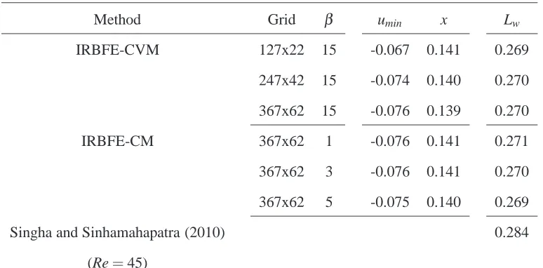
Table 6: Flow past a circular cylinder in a channel, γ =0.5, Re=60: minimum velocity uminand its position on the centreline, and the length of recirculation zones

behind the cylinder (Lw). It is noted that the case of Re=60 andγ=0.5 here is

equivalent to the case of Re=45 andγ=0.5 in Singha and Sinhamahapatra (2010).

Method Grid β umin x Lw

IRBFE-CVM 127x22 15 -0.067 0.141 0.269

247x42 15 -0.074 0.140 0.270 367x62 15 -0.076 0.139 0.270

IRBFE-CM 367x62 1 -0.076 0.141 0.271

367x62 3 -0.076 0.141 0.270 367x62 5 -0.075 0.140 0.269

Singha and Sinhamahapatra (2010) 0.284

Ω

Semi−interior element Interior grid node

Interior element

Boundary node

η

φ1 φ2

∂φ1

∂η ∂φ∂η2

x y

ΓP ΩP

N

S

W P E

n

s

e w

0 1 2 3 4 5 6 x 104 10−9

10−8 10−7 10−6 10−5 10−4 10−3 10−2

Scheme 1

Without upwinding

Number of time steps

C

M

0 1 2 3 4 5 6 7 x 104 10−9

10−8 10−7 10−6 10−5 10−4 10−3 10−2

Without upwinding Scheme 2

Scheme 3

Number of time steps

C

M

0 1 2 3 4 5 6 7 8 9

x 104 10−9

10−8 10−7 10−6 10−5 10−4 10−3

Scheme 1

Without upwinding

Number of time steps

C

M

(a) Re=0

−0.40 −0.2 0 0.2 0.4 0.6 0.8 1 0.1 0.2 0.3 0.4 0.5 0.6 0.7 0.8 0.9 1 Present (9x9) Present (11x11) Present (21x21) u y

0 0.2 0.4 0.6 0.8 1 −0.5 −0.4 −0.3 −0.2 −0.1 0 0.1 0.2 0.3 0.4 0.5 Present (9x9) Present (11x11) Present (21x21) x v

(b) Re=100

−0.40 −0.2 0 0.2 0.4 0.6 0.8 1 0.1 0.2 0.3 0.4 0.5 0.6 0.7 0.8 0.9 1 [*] [**] Present (9x9) Present (11x11) Present (21x21) u y

0 0.2 0.4 0.6 0.8 1 −0.5 −0.4 −0.3 −0.2 −0.1 0 0.1 0.2 0.3 0.4 0.5 [*] [**] Present (11x11) Present (21x21) Present (31x31) x v

(c) Re=400

−0.40 −0.2 0 0.2 0.4 0.6 0.8 1 0.1 0.2 0.3 0.4 0.5 0.6 0.7 0.8 0.9 1 [*] Present (21x21) Present (41x41) Present (61x61) u y

0 0.2 0.4 0.6 0.8 1 −0.5 −0.4 −0.3 −0.2 −0.1 0 0.1 0.2 0.3 0.4 0.5 [*] Present (21x21) Present (41x41) Present (61x61) x v

(a) Re=1000

−0.40 −0.2 0 0.2 0.4 0.6 0.8 1 0.1 0.2 0.3 0.4 0.5 0.6 0.7 0.8 0.9 1 [*] [**] 31x31 61x61 91x91 u y

0 0.2 0.4 0.6 0.8 1 −0.6 −0.5 −0.4 −0.3 −0.2 −0.1 0 0.1 0.2 0.3 0.4 [*] [**] 31x31 61x61 91x91 x v

(b) Re=3200

−0.50 0 0.5 1

0.1 0.2 0.3 0.4 0.5 0.6 0.7 0.8 0.9 1 [*] Present (91x91) u y

0 0.2 0.4 0.6 0.8 1 −0.8 −0.6 −0.4 −0.2 0 0.2 0.4 0.6 [*] Present (91x91) x v

(a) Re=0, 61×61

ψ ω

(b) Re=100, 61×61

ψ ω

(c) Re=400, 71×71

ψ ω

(a) Re=1000,81×81

ψ ω

(b) Re=3200,91×91

ψ ω

0 500 1000 1500 2000 2500 3000 3500 10−9

10−8 10−7 10−6 10−5 10−4 10−3

Scheme 1

Without upwinding

Number of time steps

C

M

0 0.5 1 1.5 2

x 104 10−9

10−8 10−7 10−6 10−5 10−4 10−3 10−2

Scheme 3

Without upwinding

Number of time steps

C

M

−1.5 −1 −0.5 0 0.5 1 1.5 2 2.5 3 3.5 −0.5

0 0.5

(a)γ=0.3

x

y

−1.5 −1 −0.5 0 0.5 1 1.5 2 2.5 3 3.5 −0.5

0 0.5

(b)γ=0.5

x

y

−1.5 −1 −0.5 0 0.5 1 1.5 2 2.5 3 3.5 −0.5

0 0.5

(c)γ=0.7

x

y

−1.5 −1 −0.5 0 0.5 1 1.5 2 2.5 3 3.5 −0.5

0 0.5

(a)γ=0.3

x

y

−1.5 −1 −0.5 0 0.5 1 1.5 2 2.5 3 3.5 −0.5

0 0.5

(b)γ=0.5

x

y

−1.5 −1 −0.5 0 0.5 1 1.5 2 2.5 3 3.5 −0.5

0 0.5

(c)γ=0.7

x

y

−1.5 −1 −0.5 0 0.5 1 1.5 2 2.5 3 3.5 −0.5

0 0.5

(a)ψ

x

y

−1.5 −1 −0.5 0 0.5 1 1.5 2 2.5 3 3.5 −0.5

0 0.5

(b)ω

x

y

−1 −0.5 0 0.5 1 1.5 2 2.5 −0.5

0 0.5

x

y

0 0.2 0.4 0.6 0.8 1 −0.2

0 0.2 0.4 0.6 0.8 1

Re=0 Re=25 Re=35 Re=60

x/D−0.5

u