Mapping changes in landscape-scale patterns of vegetation in coal seam gas development areas

(1)

Scale Patterns of Vegetation in

Coal

Seam Gas Development Areas

Final Dissertation

ENG4111/ENG4112 – Engineering Research Project Part 1 and 2 The University of Southern Queensland

Prepared By: Andrew Grigg

Candidate for the Bachelor of Engineering (Honours) (Environmental)

Supervisor:

Associate Professor Armando Apan

Submission Date: 30 October 2014

(2)

Abstract

In the 15 years to 2013, the rate of coal seam gas (CSG) development in Queensland increased dramatically. Drilling of gas wells and installation of associated infrastructure sometimes requires the removal of vegetation. Although a change in vegetation cover on a small scale does not necessarily correspond to significant landscape-‐scale change, research overseas indicates that the extent and configuration of vegetation patches in a landscape is altered in areas of concentrated oil and gas extraction. The focus of previous research has been on oil and shale gas activity, mainly in North America. There has been little work on the nature and extent of the impact of similar developments in an Australian context, or impacts due specifically to CSG activity anywhere in the world.

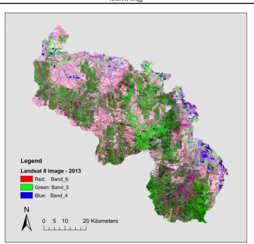
The aim of this study is to determine the nature of land cover change in a region of southern Queensland under intense CSG development. The extent and fragmentation of vegetation in 1999, immediately before CSG development began, is compared to the extent and fragmentation of vegetation in 2013, after 1562 coal seam gas wells had been drilled. Land cover was determined by classification of a LANDSAT 4 image taken in 1999 and a Landsat 8 image taken in 2013. ArcGIS 10.2 was used for image manipulation, and vegetation patch metrics were determined using FRAGSTATS 4.2 software. For comparison, the same metrics were also calculated in hot spot regions defined in two different ways to focus more closely around drilling sites. Similarly, the same metrics were calculated on a classified image modified to ensure that known linear clearings were continuously defined despite the automatic classification.

(3)

University of Southern Queensland

Faculty of Health, Engineering and Sciences

ENG4111/ENG4112 Research Project

Limitations of Use

The Council of the University of Southern Queensland, its Faculty of Health, Engineering & Sciences, and the staff of the University of Southern Queensland, do not accept any responsibility for the truth, accuracy or completeness of material contained within or associated with this dissertation.

Persons using all or any part of this material do so at their own risk, and not at the risk of the Council of the University of Southern Queensland, its Faculty of Health, Engineering & Sciences or the staﬀ of the University of Southern Queensland.

(4)

University of Southern Queensland

Faculty of Health, Engineering and Sciences

ENG4111/ENG4112 Research Project

Certiﬁcation of Dissertation

I certify that the ideas, designs and experimental work, results, analyses and conclusions set out in this dissertation are entirely my own eﬀort, except where otherwise indicated and acknowledged.

I further certify that the work is original and has not been previously submitted for assessment in any other course or institution, except where speciﬁcally stated.

Andrew Grigg

0061056646

(5)

Acknowledgments

(6)

List of Tables

Table 1: Matrix showing the choice of fragmentation metrics used in other studies of landscape change due to oil and gas

development ... 23

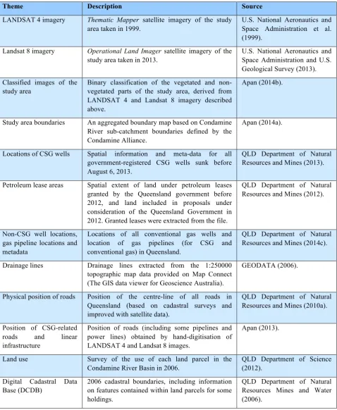
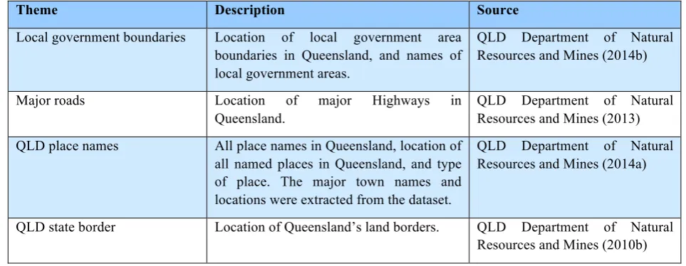
Table 2: Datasets used in the analysis. ... 29

Table 3: Datasets used to build the context map in Figure 1 ... 30

Table 4: Patch metrics considered in this study ... 37

Table 5: Land cover change matrix for the total study area ... 46

Table 6: Fragmentation metrics for the total study area ... 46

Table 7: Land cover change matrix for land under granted petroleum leases within the study area in 2012 ... 47

Table 8: Fragmentation metrics for areas under granted petroleum leases within the study area in 2012 ... 47

Table 9: Land cover change matrix for parts of the study area within 2km of a CSG well and within the study area. ... 48

Table 10: Fragmentation metrics for parts of the study area within 2km of a CSG well and within the study area ... 49

(10)

Table 12: Fragmentation metrics for the areas under granted petroleum leases in 2012, with cells through which roads run designated as "cleared" ... 50

(11)

List of Figures

Figure 1: Map showing the study area in its regional context. ... 28

Figure 2: LANDSAT 4 imagery of the study area taken in 1999 ... 30

Figure 3: Landsat 8 imagery of the study area taken in 2013 ... 31

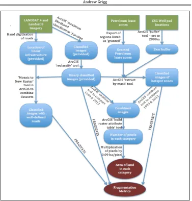
Figure 4: Flow chart showing scheme of analysis ... 33

Figure 5: Map showing regions of persistence, gain of woody cover and loss of woody cover ... 35

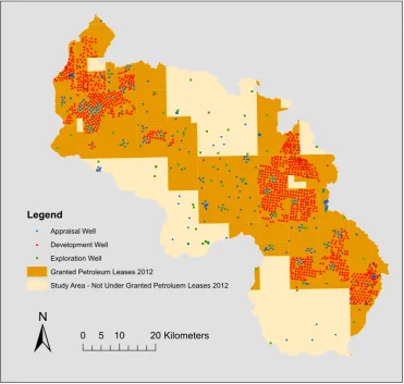
Figure 6: Regions within the study area under Granted Petroleum Leases in 2012 ... 39

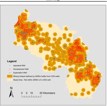
Figure 7: Regions within the study area within 2km of a CSG well in 2013 ... 40

Figure 8: Comparison of a part of the study area showing the original 2013 classified region on the left (8a), and the same region in 2013 after cells containing identified roads were designated “cleared” on the right (8b). ... 41

Figure 9: Map of linear infrastructure (labelled as roads) in the study area in 2013, overlaid with roads in the study area in 1999. ... 45

Figure 10: Graphical representation of the gross and net gain and loss of vegetated land cover between 1999 and 2013 ... 52

Figure 11: Number of patches in each tested region ... 55

(12)

Figure 13: Coefficient of variation in mean patch area in each tested

region ... 58

Figure 14: Edge density in all tested regions ... 60

Figure 15: Core area density in each tested region ... 62

Figure 16: Increase in core area density for each region tested ... 62

Figure 17: Density of disjunct core areas in each tested region ... 64

Figure 18: Shape index in each tested region (1999 and 2013). ... 66

Figure 19: Coefficient of variation of shape index in all regions tested ... 66

Figure 20: Euclidean nearest neighbour distance in each tested region ... 68

Figure 21: Coefficient of variation in Euclidean nearest neighbour distance for patches in all tested regions ... 69

Figure 22: Map showing regions of persistence, gain of woody cover and loss of woody cover, with points of interest included in the discussion ... 70

(13)

1 Introduction

1.1 Introduction

Gas production is a prominent industry in Queensland. While almost 30% of Australia’s CSG reserves are found in the Bowen and Surat basins of southern Queensland, the industry has not developed until recently (Australian Energy Regulator 2013). However, the rate of CSG development in Queensland during the decade-‐and-‐a-‐half to 2013 was very high. Currently 22.5% of CSG production for the domestic market occurs in the Bowen and Surat basins (Australian Energy Regulator 2013; QLD Department of Natural Resources and Mines January 2014). CSG and conventional gas produced in Queensland is sold exclusively to the domestic market, including for production of electricity. Exports of gas are expected to begin in 2014, with subsequent increasing capacity for export (Australian Energy Regulator 2013). Development of CSG in the Surat basin will be a major contributor to the supply of gas for export through the Queensland Curtis Liquid Natural Gas project (QGC Limited 2009b).

(14)

1.2 The Organisation of the Report

The report is broken into six major chapters: an introduction to the topic, review of literature, description of methods, results, discussion and conclusion. The introductory chapter provides:

• A background to the topic, including a statement of the problem,

• A description of the significance of the study,

• The objects of the study,

• A definition of the project scope, and consequently, the limitations on the conclusions drawn from the study.

In Chapter 2, significant literature on the topic is reviewed, creating a nest for this study. Literature on disturbance due to oil and gas extracting activity, methods of assessing land cover extent and configuration and the importance of edge and barrier effects are considered in the literature review. Chapter 3 provides a description of methods employed including an introduction of the specific study area, a justification of the chosen methods of data analysis and an outline of the resources. Chapter 4 outlines the results of the project, leading into a discussion and analysis of the results in Chapter 5. Conclusions are drawn in Chapter 6.

1.3 Statement of the Problem

(15)

taken in 1999, during the earliest developments of the industry in Australia, and Landsat 8 images taken in 2013, provide evidence of the scale of surface disturbances caused by CSG extraction. They may indicate the potential impacts of further development of the industry on the environment.

1.4 Significance of the Study

CSG developments are a recent and controversial addition to the energy production industry in Australia and the expansion of the industry has become a divisive issue in Australian society. However, there is limited evidence in the public domain, particularly academic literature, to support claims made by proponents and opponents of CSG extraction. This is true in Australia as well as in countries where the industry is well developed such as the USA and Canada. There is, however, very strong evidence in the literature that vegetation loss and fragmentation are major contributors to loss of biodiversity and reduced ecosystem health (Murcia 1995; Wilson, Neldner & Accad 2002). This study will provide a characterisation of landscape-‐scale change occurring in a region of Australia under heavy CSG development. It will provide an increased understanding and awareness of the true scale of the impact of gas extraction industries, and allow for better planning of future developments in Queensland and other parts of Australia.

1.5 Objectives

The objectives of this work were to:

1. Quantify the land cover change occurring in Queensland, on a landscape scale, in regions of concentrated CSG development. 2. Determine changes to the degree of fragmentation of remnant

(16)

3. Make comment on the probable relative effect of CSG activity on land cover and vegetation fragmentation change.

1.6 Scope and Limitations

There are a number of important principles that guide the design of this study. It was intended that:

• The study would only analyse the effects of CSG extraction on land cover change and fragmentation. Other environmental impacts of the industry were not considered, and the broader merits and drawbacks of the CSG industry were not analysed in the context of current stakeholder policies.

• The analysis is intended to draw general conclusions about the nature of change in the study area. Under the broad approach, the study is able to demonstrate the plausibility of impacts to different actors in the environment. A more focused analysis would be required to determine the impacts of change on particular species or ecological groups.

• The study focused on a binary classification of vegetated and non-‐ vegetated areas. The vegetated areas can be further classified into vegetation sub-‐types. While it is unclear how fragmented individual types of vegetation were at the commencement of CSG development, a study such as that conducted by Finn and Knick (2011) could reconstruct a historical landscape as a baseline to analyse the impact on individual vegetation types. This analysis was ruled out of the scope of the current study, but is suggested as a possible future project.

(17)

conventional gas activity occurs around Roma and Surat, and in the far South-‐West of Queensland between Eromanga and Cameron’s Corner (QLD Department of Natural Resources and Mines 2014c). Conventional gas activity in the study area was minimal, and occurred prior to 1999.

• Despite a focus on a 390,200-‐hectare region of Queensland, wider

implications for the industry in Australia are drawn from the study. Similarly, the study compares two images taken 14 years apart, but the amount of change in this time scale is intended to be relevant at other time-‐scales.

There are limitations to the methods chosen to interpret the data collected in this study. Principally, it is recognised that:

• All data has been provided by external agencies. The data is considered to be reliable, but errors or misrepresentations could impact the validity of the results of this study.

• Classification of satellite imagery is guaranteed only to 80%

accuracy. Some potential classification errors are identified in the discussion chapter.

• A generalisation algorithm is not used. Small, even single pixel, inaccuracies in classification may impact some metrics significantly, particularly those metrics that measure edge effects and core areas. These anomalies could be removed using a homogenisation technique. No such alteration was made to the data in order to preserve the impact of the small features characteristic of CSG activity on the classified image.

(18)

the results of the fragmentation analysis may only be directly compared to images in other studies that have a cell size of 30m.

• Analysis of landscape-‐wide change allows the cumulative effects of

gas extraction activities to be analysed, but land cover change due to other activities also impact on the results of the study. Analysis of hotspot areas, containing more concentrated activity, is intended to filter out some of the unrelated activity. However, it is difficult to completely isolate the impacts of a single activity when the different activities are occurring in the same space and time. Some infrastructure is developed outside hotspot areas, and other activities impacting on land cover change continue to occur within hotpot regions.

• Narrow clearings for roads and pipelines are not well represented

on the map. Tree branches may hide the full extent of a road in a satellite image. Further, the resolution of the images is 30m, in the same order of magnitude as the width of a clearing for linear infrastructure. Even single pixel discontinuities in linear clearing could have major effects on the measurement of landscape metrics. A method of forcing all cells through which roads ran to be classified as ‘non-‐forested’ cells, ensured that small linear clearings were well defined on the classified image. This transformation was successful but had the disadvantage of increasing the size of roads and removing road verge vegetation where the road raster did not align with an observed clearing exactly. The road verge vegetation is important in some parts of the study area, particularly where it exists as isolated patches.

(19)

(20)

2 Literature Review

This chapter provides a review of literature relevant to the current study. In particular, the review considers the environmental impacts of CSG, land cover change during the last two centuries in the study area, methods of land cover change analysis, landscape ecology, and various means of measuring landscape fragmentation. This chapter seeks to demonstrate the maturity of the field of landscape ecology, and draw attention to concepts that are important in the analysis of the impacts of CSG. The review also considers software and analysis techniques developed for other landscape-‐scale investigations land cover change and fragmentation, and attempts to inform the choice of techniques in this study to improve the potential for cross-‐analysis between studies.

The review shows that, while the theory of land cover change and fragmentation is well developed, it has not been widely applied to landscapes impacted by oil and gas development. Of particular interest in the review are CSG developments, on which there has been no publically available research completed in Australia. Research on the more developed industry in North America is limited, and of unknown applicability in an Australian context. Some studies on similar industries such as shale gas, and conventional oil extraction are available in the academic literature. These studies are significant for comparison in a land-‐cover study, as all forms of gas extraction activities require relatively small but interconnected production sites scattered throughout a production basin.

2.2 Gas Extraction

(21)

seams, by the removal of water, allows gas to flow to the surface through production wells (Hamawand, Yusaf & Hamawand 2013). In some cases, more gas may be retrieved from wells by physically and chemically increasing the porosity of the coal stratum. This is a process known as ‘fracking’ (Bradd et al. 2013). The gas contains a very high percentage of methane (~95%), which is used domestically or exported as Liquefied Natural Gas (LPG) (Hamawand, Yusaf & Hamawand 2013).

Primarily, CSG available for extraction occurs in large quantities in the Surat and Bowen Basins of Queensland with smaller quantities in the Gunnedah and Sydney Basins in New South Wales (Williams, Milligan & Stubbs 2013). CSG production occurs in a number of countries. At the turn of the millennium, CSG reserves were relatively undeveloped in Canada, though the industry in the USA was well established (Griffith & Severson-‐Baker 2003). Major investment in Australia’s CSG industry began in the late 90s, and the industry in Australia has developed rapidly in the last 15 years. In 1999/2000, in Queensland, fewer than 50 wells were drilled annually, but the number has risen to more than 1300 wells annually in 2012/2013 (QLD Department of Natural Resources and Mines January 2014). In 2012/2013, coal seams in Queensland yielded 7057.68 Mm3_{of gas, with production solely from the Surat and Bowen}

Basins (QLD Department of Natural Resources and Mines January 2014).

While CSG is economically important, various environmental issues are attributed to CSG extraction. These include:

• Loss of vegetation (Finn & Knick 2011; Fisher 2001),

• Habitat fragmentation (Finn & Knick 2011; Griffith & Severson-‐ Baker 2003),

• Disturbance by noise (Finn & Knick 2011; Fisher 2001; Griffith & Severson-‐Baker 2003),

(22)

• Emissions of greenhouse gasses (Fisher 2001; Griffith & Severson-‐ Baker 2003; Hamawand, Yusaf & Hamawand 2013),

• Release of co-‐produced water containing toxic chemicals or a chemical composition different to surface and ground receiving waters (Finn & Knick 2011; Fisher 2001; Griffith & Severson-‐ Baker 2003; Hamawand, Yusaf & Hamawand 2013; McBeth, Reddy & Skinner 2003),

• Depletion of aquifers (Finn & Knick 2011; Fisher 2001),

• Pollution of aquifers by methane (Fisher 2001),

• Cross-‐aquifer contamination (Bradd et al. 2013), • Soil erosion (Finn & Knick 2011),

• Invasion by exotic species (Drohan et al. 2012; Finn & Knick 2011); and

• Creation of an environment friendly to disease vectors

(particularly detention basins) (Finn & Knick 2011).

Each of these potential impacts must be monitored using unique approaches. All, but landscape fragmentation, are outside the scope of this project. This study will consider the effects of CSG on broad-‐scale surface vegetation patterns.

2.3 Historical Land Cover and Landscape Structure Change in the Study Area

(23)

Neldner & Accad 2002). A number of the vegetation types are now considered to be under-‐represented in remnant native vegetation (Seabrook, McAlpine & Fensham 2006). Alluvial Open Eucalypt Woodland and Acacia Forest have been cleared to a greater extent than Dry Eucalypt Woodlands (Seabrook, McAlpine & Fensham 2006; Wilson, Neldner & Accad 2002).

Settlers initially assumed land in the Brigalow Belt in the mid-‐nineteenth century for pastoral purposes, which required minimal clearing of the landscape. Some forest was cleared for timber, and cropping was confined to small parts of the Darling Downs (Seabrook, McAlpine & Fensham 2006). Later, with the introduction of mechanised methods of clearing in the twentieth century, large areas of land throughout the Brigalow Belt could be converted to improved pastures, or cultivated land. Conversion to crops was considered ideal as regular ploughing prevented regrowth of Brigalow forest stands (Seabrook, McAlpine & Fensham 2006). Clearing was driven by social, political and economic factors, though the specific patterns of clearing are influenced by biophysical factors, particularly soil type (Seabrook, McAlpine & Fensham 2007).

(24)

2.4 Land Cover Change

The quantification of land cover change is the focus of objective one of this study. Though, worldwide, land cover change has been analysed in a variety of landscapes, post CSG landscapes are not widely considered. Some published studies on oil development in North America are relevant to compare with the results of this work. In particular, the authors of a study in Wyoming between 1900 and 2009 note that they are amongst the only researchers to consider landscape-‐scale changes in land cover due to oil and gas activity (Finn & Knick 2011). They found that 8.3% of land cover within 0.2km of an oil well had been converted to road or well pad and 97% of the development was attributable to oil and gas development (Finn & Knick 2011). Given the small size of the hotspot area defined around each well (0.2km radius), such a finding is not surprising. However, landscape wide, 0.97% of land was converted, and 20% was estimated to be due to oil development (Finn & Knick 2011).

Studies on land cover change due to shale gas development produced similar results to those presented by Finn and Knick (2011). In a study of Marcellus shale gas extraction using a predictive model in Pennsylvania, less that 1% of forest areas were predicted to be lost across the whole study under the maximum development scenario (Johnson 2010). Another predictive model for shale gas development, this time in Canada, produced the same result (Racicot et al. 2014). A third landscape-‐scale study reported total losses, but the results of this study are difficult to use because scale of the losses was not well communicated, and loss of core forest to edge forest was not considered (Drohan et al. 2012).

(25)

gas and coal seam gas wells, through CSG well pads are noted to be smaller than shall gas well pads. In another Pennsylvanian study, shale gas well pads occupy 3.1 ha, and the average disturbance due to all infrastructure was estimated to be 8.8 ha per well (Johnson 2010). Bergquist et al. (2007) quote 1.6 ha as a typical area of disturbance (including associated infrastructure), but take the figure from a magazine article in which the source is not cited. The same magazine article suggests that well density is approximately one in every 32 ha (Clifford 2001). Williams, Milligan and Stubbs (2013) take their estimations from Broderick et al. (2011) who found that shale gas well pads alone may occupy at least 0.4 ha (if reclaimed), and may occupy more than 2 ha. Other sources estimate well pads between 1.2 ha and 2.0 ha (Drohan et al. 2012). Future development is likely to require lower well pad density (Williams, Milligan & Stubbs 2013).

Within the study area, QGC are the largest operator of CSG wells. The company is in the process of expanding operations as part of the Queensland Curtis Liquid Natural Gas (QCLNG) project. These specifications have not necessarily been used in the construction of existing infrastructure, or infrastructure built by other operators, but gives an indication of the current standards for construction in Queensland. Well pads are designed to be 100m by 100m (1 ha) initially, and 80m by 60m (0.48 ha) after partial restoration (QGC Limited 2009a). These pads are smaller than those constructed overseas or analysed in the academic literature.

(26)

the use of the easements for other services (QLD Department of Infrastructure and Planning 2010). Access roads are designed to be 4m wide (QGC Limited 2009a). These facilities are to be built throughout the Walloon Fairway, part of which occurs inside the study area examined in the current study.

2.5 Transition Matrix

In studies of land cover change, a matrix is commonly used to catalogue changes in vegetation extent. The matrix is commonly known as a transition matrix, change matrix or cross-‐tabulation matrix. It is used to analyse persistence, gain and loss of area occupied by each category of land use and land cover (LULC) in a study area. In its most basic form, the matrix displays the extent of land cover (total area or percentage cover) in each category against the land cover in each category at a subsequent time snapshot. The diagonals of the matrix represent persistent land cover, and cell j,i represents land converted from category j at time one to category i at time two (Pontius, Shusas & McEachern 2004). Though the concept was in previous use, the seminal work of Pontius, Shusas and McEachern (2004) formally described the transition matrix, defined the conditions of its use, and proposed a method of differentiating random and non-‐random landscape changes.

(27)

urban landscapes. None of the studies employing a transition matrix studied the effects of extractive industries.

2.6 Impacts of Landscape Fragmentation

The impact of fragmentation on conservation outcomes for remnant vegetation is widely studied around the world. It is well recognised that quantity is not the only important factor in assessing the environmental and economic significance of remnant habitat, but that the spatial arrangement of habitat areas is also important to ecological function (O'Neill et al. 1997; Slonecker et al. 2012). Oil and gas extraction activities can significantly alter important characteristics of the spatial arrangement of remnant habitat (Slonecker et al. 2012). Fragmentation may lead to the creation of edge effects, or create barriers to migration between isolated patches. Objective number two of this work is to quantify the fragmentation of the landscape in a CSG development region in QLD, and the background understanding needed to effectively analyse landscape fragmentation is considered here.

The creation and impact of edge habitat is one of the most well-‐studied aspects of vegetation fragmentation and is considered one of the most important causes of stress on fragmented habitat (e.g. Murcia, 1995). It has been long recognised that edges of remnant vegetation are more susceptible to change from external stressors (e.g. Murcia, 1995). As such, edges may:

• Contain forests of altered structure (Slonecker et al. 2012);

• Contain greater non-‐native plant species richness and total cover than core areas (Bergquist et al. 2007);

• Provide habitat that is subject to greater predation pressures than core areas (Piper & Catterall 2004);

(28)

• Be subject to different solar radiation, wind and moisture regimes (Murcia 1995);

• Fail to preserve the ecological integrity and wild nature of the forest (Drohan et al. 2012); and

• Attract generalist species, confining specialists to core habitat areas (Farina 1998).

The other major impact of fragmentation is the isolation of stands of remnant vegetation from one another. Each population of flora and fauna separated by the barrier effect is genetically isolated from others and less resilient to environmental stressors (Coffin 2007; Forman & Alexander 1998). Also, these populations must rely solely on habitat within an individual patch, which may or may not be of sufficient size to address their needs. Any land cover that is hostile for a species may provide a barrier to its migration between patches of remnant vegetation.

(29)

While the body of literature concerning landscape fragmentation is large, much of the data is highly species specific. It is well recognised that the analysis of landscape fragmentation is most relevant when applied to specific species (Saura & Torné 2009). Each species of plant and animal is affected by habitat isolation and edge effects according to their own characteristics, their interaction with the environment and their ability to adapt to a new environment. For example, above-‐ground pipelines have been demonstrated to prevent migration of large fauna in Canada (Dunne & Quinn 2009), and the size of non-‐forested barriers are strongly correlated to the ability of koalas to survive in small fragmented habitat areas (McAlpine et al. 2006), but these barriers don’t prevent the movement of all species. It may be possible to predict species placed most at risk through a particular change to the landscape structure by studying parameters such as population size, stability in population size, dispersal ability between patches, reproductive potential and individual area requirements (Henle et al. 2004).

It is because each species reacts to environmental change differently that defining the impacts on individual species has been ruled out of the scope of this project. Instead, this work will take a general approach used by other authors whose aim is to characterise the impacts of oil and gas development generally at a landscape scale (Baynard 2011; Drohan et al. 2012; Finn & Knick 2011; Racicot et al. 2014; Slonecker et al. 2012). This study will analyse landscape change by considering a number of ecologically significant fragmentation metrics. Rather than assessing the implications of change for arbitrary species, ecosystems or vegetation types, it will draw general conclusions about whether or not significant impacts on some populations are plausible in Queensland.

(30)

concerning fragmentation effects of other oil and gas extraction industries in North America are useful for comparison, the current work is important in the context of CSG development and for an Australian perspective. A number of the studies from North America have taken a predictive or a retrospective approach, to determine the future or past impact of oil and gas extraction industries on landscape structure (Drohan et al. 2012; Finn & Knick 2011; Johnson 2010; Racicot et al. 2014; Slonecker et al. 2012). Each of these studies demonstrates that relatively minor losses of overall vegetation may coincide with major changes in the landscape fragmentation metrics. This finding is particularly relevant in the fulfilment of objective three of this study. Other potentially relevant bodies of work analyse the impacts of disturbance on remnant vegetation, though not necessarily due to oil and gas extractive industries. Of particular relevance to this study are the impact of roads and edge effects on vegetation (Collard, Le Brocque & Zammit 2011; Finn & Knick 2011; Murcia 1995; Neel, McGarigal & Cushman 2004; Reed, Johnson-‐Barnard & Baker 1996).

Many of the studies that measure fragmentation in regions of concentrated gas extraction have been conducted in Pennsylvania (Drohan et al. 2012; Johnson 2010; Slonecker et al. 2012). In one such study of infrastructure development for conventional natural gas extraction, the development removed double as much interior forest as forest lost overall, and created as much forest influenced by edge effects as forest lost overall (Slonecker et al. 2012). Similarly, Drohan et al. (2012) studied fragmentation due to shale gas development in Pennsylvania. Some direct loss of core forest areas was identified due to shale gas development, but landscape structure metrics and losses to edge forest were not analysed.

(31)

differences in management of wells on public and private land in Pennsylvania. Abandonment of agricultural land surrounding shale gas development areas was hypothesised, as occurs in rural areas that are fragmented by urban development (Drohan et al. 2012). Griffith and Severson-‐Baker (2003) also briefly considered the impacts on agriculture, but the firm focus of the literature is on fragmentation in forested areas, particularly core forests. Drohan et al. (2012) also considered the impact on streams by measuring the average distance between well pads and watercourses, though the distances were not quoted.

Drohan et al. (2012) were a major influence on a similar study in Canada that assessed previously fragmented regions using predictive models for shale gas development. While forest areas were predicted to reduce by <1% across the whole study area there was predicted to be an increase in the number of forest patches of up to 21%, and a decrease on forest patch size by approximately 10% (Racicot et al. 2014). Much of the impact was due to pipeline construction, which was considered to require 18m wide clearings (Racicot et al. 2014).

(32)

much smaller. A noted difficulty in this work was a lack of information on oil and gas infrastructure other than roads. In some studies, methods of predicting locations for infrastructure such as roads and pipelines were developed (Finn & Knick 2011; Racicot et al. 2014). In this study, hand digitisation of the CSG road network, used for a previous study, will allow for a more complete analysis of the impacts of all CSG infrastructure.

The impact of road density and well pad density on fragmentation was measured in a number of studies (Bi, Wang & Lu 2011; Drohan et al. 2012; Finn & Knick 2011; Racicot et al. 2014). While Drohan et al. (2012) used the length of roads constructed as a measure of fragmentation, it was Bi, Wang and Lu (2011) who demonstrated a correlation between the length of roads constructed, density of wells and landscape fragmentation in an area impacted by conventional gas extraction in China. In particular, more regular area-‐weighted mean patch shape was correlated to a greater road density and well pad density was strongly positively correlated with the number of patches.

Edge effects have been studied extensively, though not necessarily in studies related to energy extraction activities. The most relevant study of the impact of edge effects, specifically due to CSG, was completed in the Powder River Basin of Wyoming (Bergquist et al. 2007). This study did not consider the extent of fragmentation, or the specific activities that caused change, but showed that vegetation adjacent to CSG developments was altered in density and species composition. Particularly, increased invasion by non-‐native species was observed. Objective two of this study is to measure the fragmentation occurring in the study area. The research conducted by Bergquist et al. (2007) is significant because it indicates that, where fragmentation due to CSG occurs, demonstrable edge effects are plausible.

(33)

Brigalow vegetation communities in Queensland found that edge effects, in forest stands adjacent to agricultural areas, did not cause a reduction in species diversity or change in community composition, when compared to core areas of that vegetation remnant (Collard, Le Brocque & Zammit 2011). Edge effects of fragmentation may not be as significant an issue in the Brigalow Belt as in other parts of the world. Many studies reviewed by Murcia (1995) found the edge zone to be less than 50m wide, though this review found many of the studies not to be rigorous enough to analyse the complexities of edge effects, to study the effects at a fine enough scale or to make general conclusions about the principles of edge effects. Despite the difficulty in defining and measuring edge effects, an arbitrary buffer is chosen in fragmentation studies to estimate the extent of edge effects. Some consensus has grown around an arbitrary width of 100m (Drohan et al. 2012; Racicot et al. 2014). In other studies, smaller arbitrarily chosen buffers of 50m (Reed, Johnson-‐ Barnard & Baker 1996), 60m (Finn & Knick 2011) and 90m (Neel, McGarigal & Cushman 2004) have been used.

2.8 Methods of Measuring Fragmentation

The importance of the choice of fragmentation metrics for monitoring ecological function, and the complexity in choosing appropriate metrics to measure the impacts on landscape structure, is well recognised. Metrics must be carefully chosen to be (McGarigal n.d.-‐b, n.d.-‐a; Neel, McGarigal & Cushman 2004; O'Neill et al. 1997; Slonecker et al. 2012):

• Truly indicative of the landscape;

• Applicable to the particular ecological processes under

consideration;

• Meaningful in analysis (sensitive to landscape differences but not

classification errors);

• Comparable (must be considered when comparing images of

(34)

• Not mutually correlated (mathematically by representing the same information in different ways, or empirically due to correlations in the physical landscape between factors that are evaluated by different metrics).

Despite academic attempts to develop sets of metrics that, together, are sufficient and necessary to describe a landscape, these sets of metrics have not been widely adopted (Baynard 2011; Riiters et al. 1995). Further, standards have not been developed, by industry or government, to guide the choice of metrics for investigations into habitat fragmentation due to extractive industries (Baynard 2011; McGarigal n.d.-‐a). Neel, McGarigal and Cushman (2004) suggest that metrics should be categorised on a continuum from being completely correlated to patch area to being completely correlated to aggregation, and several metrics chosen from across the continuum.

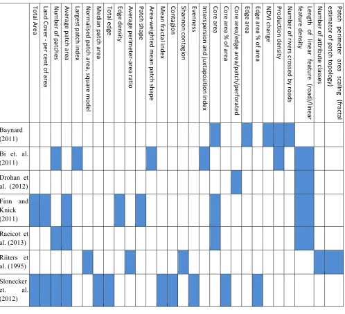
Without a common standard, the sets of metrics chosen by researchers do not match those in other similar studies. Table 1 summarises which landscape metrics have been chosen to describe fragmentation in studies on fragmentation due to gas extraction, or proposed as standard sets of metrics for that purpose. The lack of correlation between studies makes it difficult to select metrics that will allow for effective inter-‐study comparison, or to link the results of this study to others in the past. Since a large number of common class metrics show little correlation to one another and a broad understanding of landscape structure is required in this work, a fairly large number of different types of metrics will need to be calculated (Neel, McGarigal & Cushman 2004).

(35)

Table 1: Matrix showing the choice of fragmentation metrics used in other studies of landscape change due to oil and gas development

To

tal

A

re

a

La

nd

C

over

-‐ p

er

ce

nt

of

are

a

Nu

m

be

r o

f p

atc

he

s

Av era ge p at ch ar ea La rges

t p

at ch in dex No rm alis ed p atc

h a

re

a, s

qu

are

m

od

el

Me dian p at ch are

a

To

tal

e

dg

e

Ed

ge

d

en

sit

y

Av era ge pe rim ete r-‐ar

ea

rat io Pat ch sha pe Ar ea -‐we igh te

d m

ea

n p

atc

h

sha pe Me an fr ac ta

l inde

x

Cont ag ion Sh an no

n c

ont ag ion Ev en ne

ss

In

te

rsp

ers

io

n a

nd ju xta po sit io

n i

nde

x

Cor

e a

re

a

Cor

e a

re

a %

of

are

a

Cor

e a

re

a/

edg

e a

re a/ pa tc h/ pe rfo ra te

d

Ed ge ar ea Ed ge ar

ea

%

o

f a

re

a

NDVI ch an ge Pr od uc tio

n d

en

sit

y

Nu

m

be

r o

f r

ive

rs c

ro

sse

d b

y r

oa

ds

Len

gt

h

of

lin

ea

r

fe atu re (ro ad )/ lin ea

r

fe atu re de ns ity Nu m be

r o

f a

ttr

ib

ute

cla

sse

s

Pat ch per im et er ar

ea

sc

al

in

g

(fr ac tal es tim at or o

f p

at ch to po lo gy) Baynard (2011)

Bi et. al. (2011)

Drohan et

al. (2012)

Finn and Knick

(2011)

Racicot et

al. (2013)

Riiters et

al. (1995)

Slonecker

et. al.

(2012)

2.9 Software Tools for Measuring Fragmentation

[image:35.595.63.562.120.574.2]

(36)

(McGarigal n.d.-‐a). One application of FRAGSTATS is in the assessment of the impacts of extractive industries on landscape vegetation fragmentation. In this field of study the software has been applied to research on natural gas extraction in Pennsylvania (Slonecker et al. 2012), oil and natural gas development in Wyoming (Finn & Knick 2011) and oil extraction in China (Bi, Wang & Lu 2011).

Many software options are available, and the development of new tools is a continuing field of development (Saura & Torné 2009). Other recent land cover fragmentation studies have used ATtILA, which is an extension to ArcView developed by the USEPA (Slonecker et al. 2012), or have used spatially implicit models of landscape metrics. The implicit models have been superseded by spatially-‐explicit GIS models such as those used by FRAGSTATS (Didham & Ewers 2012; Racicot et al. 2014). FRAGSTATS is considered a good choice for the current study because of its previous widespread use, versatility and applicability.

2.10 Summary

The academic basis for a study of land cover and fragmentation change is well established. Research in landscape ecology has established the importance of extensive and appropriately arranged remnant vegetation for the survival of flora and fauna populations and the overall health of the environment. Further, the regions of Queensland under heavy CSG development are already at high risk due to their history of disturbance. Various tools have been established to analyse land cover change and fragmentation, including theoretical methods (e.g. land cover matrices and fragmentation metrics) and software (e.g. ArcGIS and FRAGSTATS). These tools are well tested, reliable, and readily applied in this study, although there is a lack of consensus around the choice of fragmentation metrics to use in a study such as this.

(37)

(38)

3 Methods

The ‘Methods’ chapter provides a description of the means by which this research was undertaken. It includes a description of the study area, sources of data, empirical and statistical methods. Each of the choices made in designing the experiment are justified, particularly where there is divergence from the methods used in other similar studies, or a lack of consensus in the methods used by other researchers.

3.2 The Study Area

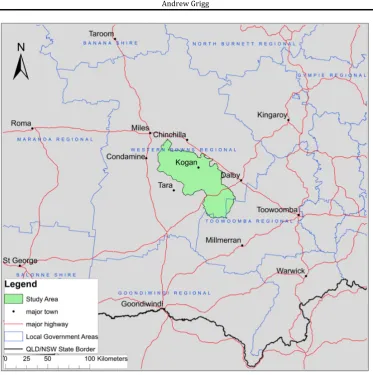
The study area has been chosen to include some of the most heavily developed CSG fields in Australia. It is shown in its regional context in Figure 1. The defined area covers 3.902×105_{hectares in southern}

Queensland, mostly in the Western Downs Regional local government area and partially in the western parts of the Toowoomba Regional local government area. The region is bounded by the parallels S 26°43’, S 27°35’, E 150°17’ and E 151°12’, includes the township of Kogan, and is close to Dalby and Chinchilla. It is wholly within the Condamine River catchment, and has boundaries defined by the extent of a number of major co-‐adjacent sub-‐catchments (Wieambilla Creek, Wilkie Creek, Braemar Creek, Kogan Creek and Wambo Creek). The Condamine River itself roughly defines the northern boundary of the study region.