Maximization of Per Node
Throughputfor2HR-Manets under Limited Buffer Constraint
B. BasaveswaraRao, SK. MeeraSharief, K. GangadharaRao, K Chandan
Abstract: This paper proposes an analytical framework on the lines of Jia Liu et al for maximization of per node throughput under limited buffer constraint of two hop relay (2HR) MANETs. To achieve maximization of per node throughput through partial derivative method with necessary and sufficient conditions (NSC) based search algorithm for finding the optimal values of network control parameter, buffer size at source node and buffer size at relay node. The per node throughput is evaluated through NSC search algorithm for different values of packet generating probability, area of the MANET and node density. The numerical results illustrate the effects of different network parameters on throughput performance.
Keywords: 2HR, Source Buffer, Relay Buffer, Node Density, Throughput.
I. INTRODUCTION
The technological developments in Internet and wireless communications have increased exponentially over last two decades.Due to mobility of devices there is a necessity to investigate theMobile Ad Hoc Network,which is being a infrastructure less, wireless network without centralized administration. In such type of networks the mobility of nodes depends on the different parameters such as mode of mobility of users, mechanism of forwarding packets and node density. The real time applications of MANETs are military, disaster relief, rescue applications and border communication during war time etc.
The commercialization of MANET can be achieved by two fold 1. With thorough understanding of node mobility, routing mechanism, congestion control, security mechanisms etc., through real timeapplications. 2. To achieve the customized MANETs with better QOS metrics.One of the major research problem in MANETs is the packet dropping which would be directly or indirectly effecting the important QOS metrics of MANETs there is always a possibility to create some buffer space at individual node so that the packet would not get dropped, instead they get stored in buffer space.
Revised Manuscript Received on May 06, 2019
B. BasaveswaraRao, Department of Computer Science and
Engineering, AcharyaNagarjuna University, Guntur, India
SK. MeeraSharief ,Department of Computer Science and Engineering,
GIET College of Engineering, Rajahmundry, India.
K. GangadharaRao, Department of Computer Science and
Engineering, AcharyaNagarjuna University, Guntur, India
K Chandan, Department of Statistics, AcharyaNagarjuna University,
Guntur, India
In the real time usage of MANETs, the existence of finite buffer at each node is quintessential characteristic for their basic existence would be the main contribution for optimizing QOS parameters. The quantification of QOS metrics in the context of infinite buffer size is not appropriate and there would not be any accuracy in doing so.
From the last two decades several researchershave derived the QOS metrics for finding parameters in MANETs using queuing models. SaadTalib has developed queuing approach to model the MANET performance using two queuing mechanisms as Drop Tail and REM for different queuing parameters and observed the REM performed well in each observation for infinite buffer. Ahyoung Lee and Iikyeun Ra have developed a queuing network model for multimedia communication using adoptive-gossip algorithm for maximizing the achievable throughput for infinite buffer. Michael J.Neely and EytanModianohave drawn exact expressions for network capacity and also fundamental rate delay curve.All the researchers aforementioned have assumed infinite buffer which never had any considerable bearing on optimizationofQoS Parameters because of the implicit assumption thatthe dropping probability is zero.Jia Liu and Yang Xu have performed the modeling for MANETs under general limited buffer constraints and resource allocation for throughput optimization using b/b/1/k Bernoulli process and theoretically modeled. Jia Liu and Yang Xuhavedeveloped a general theoretical framework and determined the end to end delay using basic probabilities of two hop relay network.Hiroki Takakura and Ruo Ando have studied throughput optimization for 2HR MANET under the general buffer constraint and derived the exact expressions for per node throughput. B.BasaveswaraRao and SK.MeeraSharief have compared the routing protocols of MANET and found the optimal protocol in terms of performance and also investigated the impact of mobility patterns on different routing protocols in MANETs with and without buffer schemes and discussed the observations in both the schemes.
All the above mentioned research contributions are related to MANET QOS measures like dropping probability for both with and without buffers. But these contributions have never focused on optimizing the routing control parameter, buffer sizefor throughput maximization involved in packet transmission process, under different network areas for new packet arrivals or relay
Maximization of Per Node Throughputfor2HR-Manets under Limited Buffer Constraint
maximization is to identify the MANET efficiency.
There is a need to achieve maximize the throughput with buffer optimization and routing control.To fill this gap and to achieve this objective the analytical study is proposed on the line of[9, 10].
The main objectives and contributions of this paper are as follows:
To derive a better procedure than earlier contributions of [9,10] optimal values for the routing control parameter, source and relay buffer values.
In this direction a specific set of necessary and sufficient conditions are derived through partial derivative method.
To provide a search algorithm for finding the optimal values for maximization of per node throughput.
The numerical illustration is presented for supporting this process and drawn conclusions.
The remaining part of thispaper is organized as follows. Section 2 is discussed about the related work with limited buffer in MANETs by taking different performance metrics withan intent towards buffer and service optimization. Section 3 clearly discusses about the preliminaries of the system and the respective parameter definitions and derivations. Methodology, Exact expressions and derivations for enhancement of buffer, routing control parameter andmaximization of throughputusing a novelistic algorithm and different derivations are presentedin section 4.In section 5numerical illustrationsof the network setting parameters and initial values are provided. Results and discussions are presented.These were illustrated and examined deeply in section 6.Finally the conclusions and future scope of the work are presented in section 7.
II. RELATED WORK
A significant amount of research work has been published earlier in the area of performance analysis of MANETs through analytical and simulation studies. Some of the research works mentioned below related to the queuing model based performance metrics with buffer and without buffer at each node of the MANET.
F.R.B. [1] Cruz et al have developed a multi objective approach for the buffer allocation and throughput tradeoff problem for single server queuing model for Generalized Expansion Method through Multi Objective Genetic Algorithm and found the optimal solutions. A.Lee and I.Ra [2] have proposeda queuing network model based on adoptive-gossip algorithm with loss probabilityfor reducing the routing load. Mouna A and Mounir F et al [3] have improved the performance of delay tolerant mobile networks using mobile relay nodes under general buffer constraint and conducted tests for different mobility models as network settings.Yujian Fang [4]etal have reported practical performance of MANETs in single server queuing theory
for buffer size, packet life time, throughput, packet loss ratio, and packet delay in a theoretical framework.
Jia Liu and Min Sheng [5]et al revealed the relationship between the throughput capacity and relay-buffer blocking probability under general buffer constraints with 2HR-α Scheme.Yin Chen [6] has derived the expressions for throughput capacity of A-MANETs and developed a theoretical framework for exact capacity evaluation for other MANET scenarios.Jia Liu and Min Sheng [7]et alhave studied a novel theoretical framework with two hop relay mobile ad hoc networks for end to end delay modeling. Wu wang and Bin yang [8] et al have studied packet delivery delay performance in three-dimensional mobile ad hoc networks using an algorithm and derived the closed-form expressions. Jia Liu and Ruo Ando [9] et al have created a theoretical framework to calculate the inherent buffer occupancy behaviors in Bernoulli process model.Jia Liu and Yang Xu [10] et al have modeled a 2 Hop Relay with routing control parameter for packet delivery in MANET under general limited buffer constraints and explored the
ideas to implement in an
experimentalsetup.B.BasaveswaraRao and
SkMeeraSharief[11] et al have performed a comparison between the routing protocols and identified the best performing protocol using a limited buffer at a random value
through simulation. SK M Sharief and B
BasaveswaraRao[12]et alhave identified the impact between the routing protocols using buffer considering the buffer value asrandomly and without buffer through simulation for different network parameters.
Ad hoc nodes should be deployed compactly to maintain a elevated extent of interaction between mobile nodes because of their limited transmission power, and many ad hoc route discovery protocols have been implemented based on simple flooding method from occasion to occasion broadcasting routing packets in all the other nodes to provide the shortest-path routing techniques and achieve a far above the ground extent of availability to set up secure routes in an optimistic way.
This paper proposes a queuing network model with B/B/1/K that maintains at each node a limited buffer B, the packet generating at each node is Bernoulli process with packet generating probability rate λ and service generating rate µ [9, 10], number of nodes in the network are “n” and area is m x m which is equally partitioned with an m2 number of cells.
III. PRELIMINARIES
A. Notations:
m: Area of the torus network
n: Number of mobile nodes in the torus network B: Size of the total buffer at each node
Bs: Size of the buffer at Source Node
Br:Size of the buffer at Relay Node
Psd:Probability that a node gets the chance to transmit the
packet fromsource to destination
Psr:Probability that a node gets the chance to transmit the
packet fromsource to relay
Prd:Probability that a node gets the chance to transmit the
packet fromrelay to destination
λs:Packet generating Probability rate at source node
µs:Packet transmission Probability rate at source node
α: Routing control mechanism parameter
πs(0):Initial probability that the packets occupying at the
source buffer
πr(i): The probability that there are i packets occupying in
the relay buffer
B. Network Model Assumptions:
The widely used network model is adopted from [6, 9, 10].The torus network area is evenly partitioned with non-overlapping cells of m x m area contains n mobile nodes randomly move in the network area following a uniform type mobility model. By using this mobility model, the location identity of node is motionless with stationary distribution uniform on the network area on theother hand routes of different nodes are independent and identically distributed. The time slotted, supports only one transmission between two nodes within the radio transmission range. The concurrent transmission of packets in different cells will not interfere with each other. There also exists more than one node in a cell. Each node in cell becomes the transmitter with equal likelihood. The maximum number of nodes in a cell is not more than three, i.e. source node, destination node and relay node. The minimum number of nodes in a cell may be zero. It means a cell may or may not contain a node.
C. Traffic Model:
Bernoulli process model is used for packet generating process at each node with a rate of λs and during a time slot
the total amount of data that can be transmitted from a transmitter to its corresponding receiver is fixed and normalized to one packet. Unicast traffic flow model is used as the traffic model in this paper [10] which is n unicast traffic flows exist in the network. In the network each node is the source of one traffic flow and meanwhile the destination of another traffic flow.
D. Buffer Model:
As illustrated in fig 1, consider that node maintains a total buffer space of B packets, which is allocated to the source buffer of size Bs and relay buffer of size Br .i.e.,
B=Bs +Br (1)
The source buffer is for storing the packets of its own flow and works as queuing mechanism in an order of first in first out (FIFO) source queue.while the relay buffer is for
storing packets of all other n-2 flows and works as n-2 FIFO virtual relay queues.
Fig1:B/B/1/BsQueuing Model for Source Buffer
E. 2HR-Routing Scheme
To support the efficient operation of a MANET under the general buffer constraint, introduced a new routing scheme and control parameter into the 2HR scheme for packet delivery and routing from the source node to destination node without loss of generality. Here a tagged flow is focused as source node to destination node as S and D respectively.Once S gets access to wireless channel at the beginning of the time slot in the torus network area of size mxm in the total nodes n.It executes the 2HR Scheme as follows.
i. If D is within the cell of S, S executes the source to destination operation.
ii. If D is not within the cell of S, S randomly selects one of the node R as relay within its cell as its receiver, it executes source to relay operation with a two way probability, and continued relay to destination operation with another way of probability.
F. Basic Probabilities :
Let Psd,Psrand Prd[9, 10] denote the basic probabilities that a
node gets the chance to transmit packet from the source to destination (S-D) , source to relay (S-R) and finally relay to destination (R-D) operations respectively and these basic probabilities are as follows
2 2
2 1 2
1
1
1
1
(
1
)
1
sd
n
m
m
m
P
n
n
n n
m
(2)1 2
2 2
2
1
1
1
1
1
1
1
n n
sr
m
m
P
n
n
m
m
(3)
2 2 1
2 2
1 1
1 1
1 ) 1
1 1
( rd
n n
m m
P
n n m m
(4)
G. Buffer occupancy process analysis
a. Source buffer :
The buffer at source node can be defined as, in every time slot a new packet is generated with probability of λsand a
service opportunity arises with probability of µs can be
determined as
µs =Psd+Psr
Maximization of Per Node Throughputfor2HR-Manets under Limited Buffer Constraint
Fig:2 Birth Death Chain Processes of State Machines
Thus, the occupancy process of source buffer can be modeled by a B/B/1/Bsqueue.Let πs (i) denote the
probability that there are i packets occupying the source buffer in the stationary state then the stationary occupancy state distribution(OSD) of the source buffer ∏s = { πs (0), πs (1),…, πs (Bs)} is given by
.
,1
.
,
0
1
1
B s
s s
Bs
s s
s
i
s s
s
s s s
i
B
i
i
(6)
(1
)
(1
)
,
s ss s
where
b. Relay Buffer:
The analysis of occupancy process of relay buffer in Source S can be determined as πr (i).Let πr (i) may denote the
probability that there are i packets occupying the relay buffer in the OSD determined as
0
(1
(0))
(1
)
,
(0)
r
B k
i i
i s
r
k k
s k
C
i
C
0
i
B
s (7)where
1
and3
.
i
n
i
i
C
From the above notations and basic definitions the following section is to improve the procedure for contributions of [9,10] the buffer size at source node, relay node, routing control parameterare optimized for maximization of per node throughput for various given values of m, n, and λs.
IV. IMPROVED DERIVATION FOR
MAXIMIZATION OF THROUGHPUT(T*) The main objective of this paper is toimprove the maximization of per node throughput of a limited buffer MANETs with 2HR schemecompared to earlier contributions of [9,10]. To achieve this objective the contributions [9, 10] have been considered and also adopt the exact derivation of per node throughput, to find the optimum values of α*, Bs*, Br* for given values of λs,m and
n.The per node throughput (T) is derived in [9, 10] as follows.
T=Psd(
1
s(0)
)+Psr(1
s(0)
(1
r(
B
r)
), (8)The authors[9,10] achieve maximization of per node throughput (T*) through optimization of α, Bs, and Br
withpartial derivative method after thengolden search algorithm is used forfinding the corresponding α*, Bs*andBr*.
This section intends to find optimal values for α*, Bs* and
Br* to maximize T* using partial derivative method andalso
to derive necessary and sufficient conditions.For this partial derivative method is used to arrive at necessary and sufficient conditions, these conditions are used as a basis to develop novel criteria based search algorithm.
If one observes the equation (8),there is a condition to be identified that the values of πs(0) and πr(Br) are minimized
then T is maximized. So for minimization of πs(0)and πr(Br),
thepartial derivative of equations (6) and (7) and equals to zero then derive the necessary and sufficient conditions withsecond order partial derivative which is positive . From these suitable necessary and sufficient conditions an algorithm is proposed for finding α*, Bs* and Br* which is
as follows.
A. Derivations Of The Necessary And Sufficient
Conditions For The Existence Of Α* And Bs*:
Let πs(0) denote the initial probability that the packets
occupying the source buffer is given in (6) then first partial derivative and second partial derivatives are given below:
( (
( (0
) (
. ) )
. ) . log ) 0
. log )
( .
0
Bs
s s s s s
s Bs Bs
s s s s
B s
s
s
s s s
Bs
s s
o o
o
o o
B
B
2
(
(
) ( .
log )
.
)
Bs
s s s s
Bs s
s s
o
B
2 2 2 2 2 2
. ) . log ) 0
. ) . log ) . log ) . (log ) ) 0
) log
. ) 2 . log
( (0
( (0 (0 (0
( (
. )
( ( )
s Bs Bs
s s s s
s Bs s Bs s Bs Bs
s s s s s s
Bs
s Bs Bs
B s
s
s s s
s s s
s s s
s s s B B o o
o o o
o o B B B 2 2 2 2 2 2 2 2 2 ( ( ( ( ) ( ( ( ( ( )
. (log ) ) 0
. )
) ( log )
. ) 2 . (log ) )
. ) . )
) (log .
. )
. ) . )
( ) 2
( ( ( Bs s s s Bs s s Bs
s Bs s s s s s Bs
s s Bs Bs s
s s s s
Bs Bs
s Bs s s s s
s s Bs Bs
s s s s s s B B o o 1
2
2
2 2
) (log .
1 . ) ( . ( ) ( ) 2 Bs Bs
s s s s s
Bs Bs
s s s s
s B o
(10)
From the equations (9) and (10) to minimizeπs(0) there must
be a second derivative which is positive and first derivative
beingzero. To observe (9) and (10) the necessary and
sufficient conditions are drawn for minimize πs(0) i.e.
2
2
and
0
0
s s s s s so
B
o
iff
B
µ
(11)( θ)Bs>0 (12)
The maximum per node throughput will be occurred when
the probability of transmission packets at source is always
greater than the probability of packet generated at source
that routing control parameter α yields optimal value. This condition θBs> 0 will exist only which B
svalue holds θBs> 0
that Bsvalue must be a optimal value of throughput
maximization where µs>λs.
B. Derivations of The Necessary And Sufficient Conditions For The Existence Of Br*:
Let πr(Br) denote the probability that the packets occupying
the relay buffer is given in (7) then first order partial derivative and second order partial derivatives are as given below: 0 0 0 ' ' 2 ' (1 (0)) (1 (0)) (1 (0)) (1 (0))
( 3 )!
(1 (0))
( 3)! !
( 3 )!
(1 (0))
( 3)! !
( 3 )!
( 3 , )! ! r r r r r r r r i i i s r k k s B B B s r r k k s B B r s r r r k k r s r r B r r r r k k B k k B k B n B n B B n B n B C i C C C A B A B B A
B B B B n A B n ' ' ' '
( 3 )!
((1 (0)) ) ((1 (0)) ) log((1 (0)) )
( 3)! !
( 3 )! ( 3 )!
((1 (0)) ) log((1 (0)) )
( 3)! ! ( 3)! !
( 3 )!
((1 (0))
( 3)! !
0
r r
r
B r B
s s s
r
B r r
s s r r r s r n B n B
n B n B
n n B
B n B
B n B '
( 3 )!
) ((1 (0)) ) log((1 (0)) )
( 3)! !
( 3 )! ( 3 )!
((1 (0)) ) log((1 (0)) )
( 3)! ! ( 3)! !
r r
r
B r B
s s
r
B r r
s s
r r
n B
n B
n B n B
n B n B
0
'
( 3 )! ( 3 )! ( 3 )! ( 3 )!
((1 (0)) ) log((1 (0)) ) (1 (0)) (1 (0)) )
( 3)! ! ( 3)! ! ( 3)! ! ( 3)! !
( 3 )!
( 3)! ! r
r r r
B r r r kk r B B
s s s s
r r r r
r B k r r k r r
n B n B n B n B
n B n B n B n B
B
B n B
n B 2 0 (1 (0)) r kk s B ' 0
( 3 )! ( 3 )! ( 3 )! ( 3 )! ((1 (0)) ) log((1 (0)) ) (1 (0)) (1 (0)) )
( 3)! ! ( 3)! ! ( 3)! ! ( 3)! !
( 3 )! ( 3) 0 . ., r r r r r r r
B r r r k k r B B
s s s s
r r r r
r B k
B B
n B n B n B n B
n B
i e
B n B n B n
n B n 2 0 0 (1 (0)) ! ! r B kk s r k B ' 0 '
( 3 )! ( 3 )! ( 3 )! ( 3 )!
((1 (0)) ) log((1 (0)) ) (1 (0)) (1 (0)) )
( 3)! ! ( 3)! ! ( 3)! ! ( 3)! !
( 3 )!
( 3)! !
r r
r
r
B r r r k k r B B
s s s s
r r r r
r r r r r B k k
n B n B n B n B
n B n B n B n B
B
B n B
n B 2 0 2 ' 0 0 ' (1 (0))
( 3 )! ( 3 )! ( 3 )! ( 3 )!
(1 (0)) ((1 (0)) ) log((1 (0)) ) (1 (0))
( 3)! ! ( 3)! ! ( 3)! ! ( 3)! !
r r r r k k s B
k k k k
r
B
B B
k
r r r
r r s s s s
r r r k r
n B n B n B n B
B
n B n B n B n B
2 '
0
' '
0 '
( 3 )!
(1 (0)) )
( 3)! !
( 3 )! ( 3 )! ( 3 )! ( 3
(1 (0)) 2 (1 (0)) .(1 (0))
( 3)! ! ( 3)! ! ( 3)! !
r r
r r r
r r r B B k BB r s r
B B BB
k k
r r r
r r s
k
r r s s
r r r
n B n B
n B n B n B n
B B
n B n B n B
)!
log((1 (0)) )(1 (0)) ( 3)! !
r r B B r s s r B
n B
0 '
( 3 )! ( 3 )! ( 3 )! ( 3 )!
1 (0)) )((1 (0)) ) log((1 (0)) ) (1 (0)) (1 (0)) )
( 3)! ! ( 3)! ! ( 3)! ! ( 3)! !
((1 ( lo
0 ) ) g
)
( r r r
r
B r r r k k r B B
s s s s s
r r r r
B
B
k
s
n B n B n B n B
n B n B n B n B
' ' 0
( 3 )! ( 3 )! ( 3 )! ( 3 )!
log((1 (0)) ) .(1 (0)) (1 (0)) log((1 (0)) )(1 (0))
( 3)! ! ( 3)! ! ( 3)! ! ( 3)! !
( 3 )! (
r r
r
r r r
B B kk B B
r r r r
s s s
r
B
s s
r r r k r
n B n B n B n B
n B n B n B n B
n B n '
( 3 )!
(1 (0)) log((1 (0)) )(1 (0)) 3)! ! ( 3)! !
r r r r
BB r B B
s s s
r r
n B
B n B
2
0 ''
' 0
( 3 )! (1 (0)) ( 3)! !
( 3 )! ( 3 )! ( 3 )! ( 3 )!
1 (0)) )((1 (0)) ) log((1 (0)) ) (1 (0))
( 3)! ! ( 3)! ! ( 3
g )! ! lo ( r r r k k r
r r s
r
B r r r kk r
s s s
r B k k r B s r n B B n B
n B n B n B n B
n B n B n B
0 ' '
(1 (0)) ) ( 3)! !
( 3 )! ( 3 )! ( 3 )! ( 3 )!
((1 (0)) ) log((1 (0)) ) .(1 (0)) (1 (0))
( 3)! ! ( 3)! ! ( 3)! ! ( 3)! !
r r
r r r
r B r k B B s r
B r r B B r
s s s s
r r r r
n B
n B n B n B n B
n B n B n B n B
' 0 '
log((1 (0)) )(1 (0))
( 3 )! ( 3 )!
(1 (0)) log((1 (0)) )(1 (0))
( 3)! ! ( 3)! !
( 3 )! ( 3 )!
2 (1 (0))
( 3)! ! (
r r
r r r r
r
r r
B B
kk
s s
B B B B
r r
r B
k
s s s
r r
B B
r r
r s
r
n B n B
n B n B
n B n B
B
n B n
' ( 3 )!
.(1 (0)) log((1 (0)) )(1 (0))
3)! ! ( 3)! !
r r r r
B B r B B
s s s
r r
n B
B n B
2 0 '' ' 0
( 3 )! (1 (0)) ( 3)! !
( 3 )! ( 3 )! ( 3 )! ( 3 )!
1 (0)) )((1 (0)) ) log((1 (0)) ) (1 (0))
( 3)! ! ( 3)! ! ( 3
g )! ! lo ( r r r kk r
r r s
r
B r r r k k r
s s s
r B k k r B s r n B B n B
n B n B n B n B
n B n B n B
0 ' '
(1 (0)) ) ( 3)! !
( 3 )! ( 3 )! ( 3 )! ( 3 )!
((1 (0)) ) log((1 (0)) ) .(1 (0)) (1 (0))
( 3)! ! ( 3)! ! ( 3)! ! ( 3)! !
r r
r r r
r B r k B B s r
B r r B B r
s s s s
r r r r
n B
n B n B n B n B
n B n B n B n B
' '
log((1 (0)) )(1 (0))
( 3 )! ( 3 )!
(1 (0)) log((1 (0)) )(1 (0)) ( 3)! ! ( 3)! !
( 3 )! ( 3 )!
((1 (0)) ) l
( 3)! ! ( 3)! !
r r
r r r r
r
B B
kk
s s
BB B B
r r
s s s
r r
B r r
s
r r
n B n B
n B n B
n B n B
n B n B
0 2 0 0
( 3 )! ( 3 )!
og((1 (0)) ) (1 (0)) (1 (0)) )
( 3)! ! ( 3)! ! ( 3 )!
2 (1 (0))
( 3)! ! ( 3 )!(1 (0))
( 3)! !
r r r r r r r B B k k k r r
s s s
r r r B B
s r kk r s B B k r B k
n B n B
n B n B n B
n B n B n B '
( 3 )! ( 3 )!
.(1 (0)) log((1 (0)) )(1 (0)) ( 3)! ! ( 3)! !
r r r r
BB B B
r r
s s s
r r
n B n B
n B n B
0 2 0 ' ''
( 3 )! ( 3 )! ( 3 )! (
1 (0)) )((1 (0)) ) log((1 (0)) ) (1 (0)) ( 3)! ! ( 3)! ! ( 3)! !
( 3 )! (1 (0)) (3)! lo ! g( r r r
B r r r kk
s s s s
r r r
kk B r s k r r B k r
n B n B n B n
n B n B n B
n B n B B ' 0 ' 3 )! (1 (0)) ) ( 3)! ! ( 3 )!
.(1 (0)) ( 3)! ! ( 3 )! ( 3 )!
((1 (0)) ) log((1 (0)) ) ( 3)! ! (3)! ! ( 3 )!
(1 ( 3)! !
r r rr r r BB r s r BB r s r
B r r
s s r B k r r r B n B n B n B
n B n B
n B n B n B
n B '
(0)) log((1 (0)) )(1 (0))
( 3 )! ( 3 )!
(1 (0)) log((1 (0)) )(1 (0)) ( 3)! ! ( 3)! !
( 3 ) ((1 (0)) )
r r
r r r r
r
BB kk
s s s
BB BB
r r
s s s
r r
B r
s
n B n B
n B n B
n B 0 0 '
! ( 3 )! ( 3 )! ( 3 )! ( 3 )!
log((1 (0)) ) (1 (0)) (1 (0)) ) 2 (1 (0))
(3)! ! ( 3)! ! ( 3)! ! ( 3)! ! ( 3)! !
(
r
r r
r r r
BB BB
kk
r r r r
s s s
B B
k k
s
r r r r r
n B n B n B n B
n B n B n B n B n B
n 4 ' 0
3 )! ( 3 )!
.(1 (0)) log((1 (0)) )(1 (0)) ( 3)! ! ( 3)! !
( 3 )! (1 (0)) ( 3)! !
rr r
r r
BB BB
r r
s s s
r r kk r s B k r
B n B
n B n B
Maximization of Per Node Throughputfor2HR-Manets under Limited Buffer Constraint
From the equations of
0
r r r B B
and
2
2 0
r r
r
B B
to
minimizeπr(Br) there must be a second derivative which is
positive and the corresponding first derivative beingzero. To
observe these equationsthe necessary and sufficient
conditions are drawn to minimize πr(Br) i.e.
2
2
and
0
0
r r r r
r r
B
B
B
B
The second order derivative always positive because the
numerator terms contains with power of 2 and logarithmic
terms and hence the numerator is always positive. The
denominator term contains with power of 4 so the
denominator is also positive. The following four necessary
and sufficient conditions are satisfied when the first
derivative is equal to zero.
CONDITION 1:
0
0
(
3
)!
(
3
)!
(1
(0))
(1
(0))
)
0
(
3)! !
(
3)! !
(
3
)!
(
3
)!
(1
(0))
(1
(0))
)
!
. .
(
3)
!
,
(
3)! !
r
r
r r
r r
B B
k k
r r
s k
s
r r
B B
k k
r r
s s
r B
B
r k
i
n
B
n
B
n
B
n
B
n
B
n
B
n
B
n
B
e
CONDITION 2:
'
'
(
3
)!
(
3
)!
log((1
(0)) )
0
(
3)!
!
(
3)!
!
(
3
)!
(
3
)!
log((1
(0)) )
(
3)!
!
(
3)!
!
r r
s
r r
r r
s
r r
n
B
n
B
n
B
n
B
n
B
n
B
n
B
n
B
CONDITION 3:
0
(
0
( )
( )
0
( )
( )
0
( )
( )
0
(1 (
1
))
0
(1 (
(
(0)))
1
)
0
)
s
s
s
s
s
s r
r
r
r
r
r s
s
r
s s
B
s s
B
s s s s
B
s s
B
s s
B
s s
B s
s
B s
B
B
B
B s
B B
B B
CONDITION 4:
( )
0
0
1
0
r
r
r
B B
B
From the above four conditions only the fourth condition is
suitable for finding the Br*value which Br value satisfies the
fourth condition is Br*.
C. Discussion on Necessary and Sufficient Conditions: From the above A and B sections the following three
necessary and sufficient conditions are derived for per node
throughput maximization.
1.µs>λs
2.(θ)Bs>0
3.(α)Br>0
To finding the optimal control parameter α*, it is a necessary and sufficient condition λs<µsfor different
network parameters m,n, µs is varied as for corresponding
Psd and Psr values. So for obtaining maximum throughput
node the α* value be identified as per the λs<µs.
The second condition (θ)Bs>0,where θ can be written as
(1
(1
)
)
1
)
(1
(1
)
(
1
)
)
(
s s
s s
s s
s s
s s s
s
The ratio of transmission probability
The ratio of generating probability
The whole power of ratio of ratios ofgenerating probability
and transmission probability to the source buffer must be
greater than zero is the optimal value of Bs*.
The third condition (α)Br>0,where α is the control parameter
is the deciding factor for the total number of relay nodes and
route discovery. The whole power of control parameter to
the relay buffer must be greater than zero is the optimal
value of Br*.
Based on these existing necessary and sufficient conditions
the following Necessary and
Search algorithm is proposed for finding T*.
The following algorithm is to find the values of α*, Bs*, Br*,
T*for given m,n,λsas follows:
D. The proposed NSC Search Algorithm for Finding
α*, Bs*, Br*, T* for given m, n, andλs
Input: {m, n, ,λs,and Tolerance ϵ }
Output: {α*, Bs*,Br*, T*}
1. Initialization: set α=0.01, Bs=1,Br=1, θc=0, αc=0,
ϵ=0.000001;
2 2
2 1 2
1
1
1
1
(
1
)
1
sd
n
m
m
m
P
n
n
n n
m
1 2
2 2
2
1
1
1
1
1
1
1
n n
sr
m
m
P
n
n
m
m
µs=psd+psr
1
)
(1
(1
)
s
B
s s
s s
2. While ( µs ≤λs) { for finding α* }
1 2
2 2
2
1
1
1
1
1
1
1
n n
sr
m
m
P
n
n
m
m
µs=psd+ psr
α=α+0.01 then goto step2
3. End while α*=α;
4. While (ϵ!= (θ c - θ 1 )){ for finding Bs*}
Bs=Bs+1
1
)
)
(1
(
s
B
s s
c
s s
θ1= θc
5. Goto step4
6. End whileBs*=Bs
7. α1=(α)Br
8. While (ϵ != (αc - α1)){ for finding Br*for given α*}
Br=Br+1
Brc
α1= αc
9. Goto step8
10. End whileBr*=Br
11. {For finding T*forCorrespondingBs*, Br* and α* of
µs}
0
*.
s s
s Bs
s s
*0
* *
(1
(0))
*
(0))
(1
r r
r
r
B s
B
k s
k r
B B
r
k k
C
B
C
1 2
2 2
2
1 1
* 1 1 1
1 1
s
n n
r
m m
P
n n m m
12. T*=Psd(1-πs(0))+Psr(1-πs(0))(1-πr(Br*);
13. Return α*, Bs*, Br*and T*;
In the above algorithm the values for α* andBs* are
calculated with two necessary and sufficient conditions of
µs>λs andθBs> 0 correspondingly. The α convergent to α*
upto the valueof λs is less thanµs i.e. the source to relay
transmission probability control parameter is α* for given λs
value. The Bs convergent to Bs* up to θBs> 0.The α* value
can be used to calculate the Br* value by applying the
condition (α)Br>0. The T* value calculated by using α*, B
s*
and Br* values. The following numerical illustration
explores this algorithm for various values of network
parameters m and n.
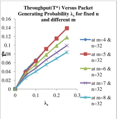
V. NUMERICAL ILLUSTRATION
Based on proposed algorithm for finding maximize the per
node throughput forgivenλsthe numerical results are
presented to illustrate the impact of λsfor different types of
Maximization of Per Node Throughputfor2HR-Manets under Limited Buffer Constraint
The numerical illustration of Throughput maximization T*
for different values of packet generating rate (λs) varies from
0.05 to 0.25 with an interval of 0.05 because the control
parameter ‘α’ value is varied from 0 to 1 as the
corresponding values of the service opportunity probability
µs, as a range from 0 to maximum of 0.3 such that the packet
generating rate is fixed as per the service probability.
Network parameters are varied in area is 4,5,6,7,8 square
meters and total number of nodes in the network are32, 50,
72, 98, 128 respectively where the NSC search algorithm
finds the corresponding control parameter α* of the torus
network, the optimized source buffer size Bs* , and the
optimized relay buffer size Br* by using these values the
maximization of per node throughput T* is derived.The
following results and discussions section explain the
different network parameters with packet generating rate
probability and also presents the dynamic behavior of
optimized routing control parameter, source and relay buffer
VI. RESULTS AND DISCUSSIONS
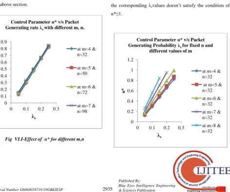
The packet generating probability is key factor to be
observed for the different cases as discussed in
[image:8.595.309.546.125.369.2]theabove section.
Fig VI.I-Effect of α* for different m,n
To observe the above graph there is no significant difference
in α* for different network parameters m, n, when λs
[image:8.595.77.549.437.831.2]increases.
Fig VI.II-Effect of α* for fixed area and various node
density
The above graph α* increasing when λs increases, for the
values of n=72, 98, 128 theα* values are greater than one, so the corresponding λsvalues doesn’t satisfy the condition of
α*≤1.
0 0.1 0.2 0.3 0.4 0.5 0.6 0.7 0.8 0.9
0 0.1 0.2 0.3
α*
λ
sControl Parameter α* v/s Packet Generating rate λs with different m, n.
at m=4 & n=32
at m=5 & n=50
at m=6 & n=72
at m=7 & n=98
0 0.2 0.4 0.6 0.8 1 1.2
0 0.1 0.2 0.3
α*
λ
sControl Parameter α* v/s Packet Generating Probability λs for fixed m and
varied n
at m=4 & n=32
at m=4 & n=50
at m=4 & n=72
at m=4 & n=98
at m=4 & n=128
0 0.2 0.4 0.6 0.8 1 1.2
0 0.1 0.2 0.3
α*
λ
sControl Parameter α* v/s Packet Generating Probability λs for fixed n and
different values of m
at m=4 & n=32
at m=5 & n=32
at m=6 & n=32
at m=7 & n=32
Fig VI.III-Effect of α* for fixed nodes and different area
The above graph α* increasing when λs increases, for the
values of m =7, 8, theα* values are greater than one, so the corresponding λsvalues doesn’t satisfy the condition of
[image:9.595.50.287.143.400.2]α*≤1.
Fig VI.IV-Effect of Bs* for different m,n.
If the packet generating rate increases then the size of the
source buffer Bsalso slowly increases uptoλs=0.15 after then
[image:9.595.308.545.401.615.2]it will steeply increasefor all the values of m, n.
Fig VI.V-Effect of Bs* for fixed nodes and different area.
When λs increases the Bs also increases and then stabilizes
for all values of m and fixed value of n.
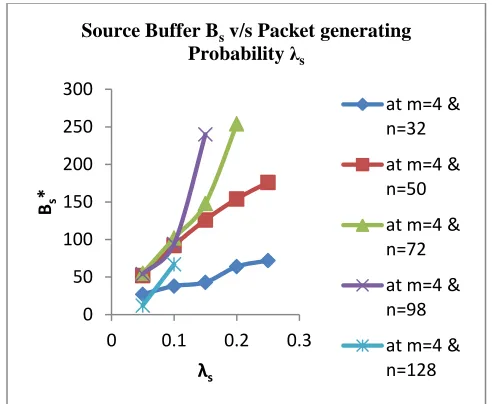
Fig VI.VI- Effect of Bs* for fixed nodes and different area
When λs increases thenBs also increases for all values of n
and fixed value of m.The demand for the increased size of
the source buffer is there when the number of nodes
areincreasing within the same torus network area.
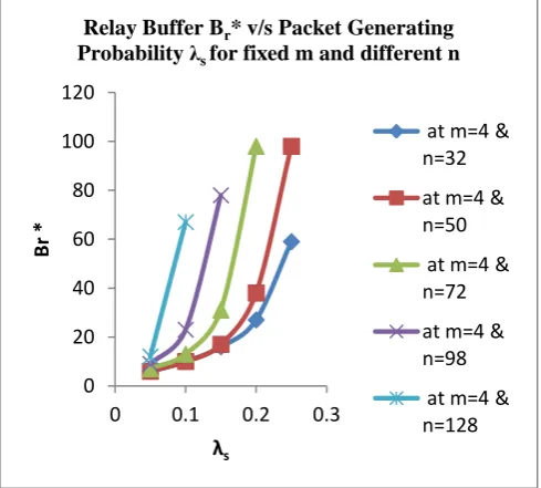
Fig VI.VII- Effect of Br * for different m, n
If the packet generating rate λs increases then gradually the
size of the relay buffer Br increases correspondingly for all
the values of m and n. 0
20 40 60 80 100 120
0 0.1 0.2 0.3
Bs
λs
Source Buffer Bs* v/s Packet generating Probability λs for different values of m,n
at m=4 & n=32
at m=5 & n=50
at m=6 & n=72
at m=7 & n=98
at m=8 & n=128
0 50 100 150 200 250
0 0.2 0.4
Bs*
λs
Source Buffer Bs v/s Packet generating Probability λs for fixed n and different
m
at m=4 & n=32
at m=5 & n=32
at m=6 & n=32
at m=7 & n=32
at m=8 & n=32
0 50 100 150 200 250 300
0 0.1 0.2 0.3
Bs
*
λs
Source Buffer Bs v/s Packet generating Probability λs
at m=4 & n=32
at m=4 & n=50
at m=4 & n=72
at m=4 & n=98
at m=4 & n=128
0 10 20 30 40 50 60 70 80
0 0.1 0.2 0.3
Br
*
λs
Relay Buffer Br* v/s Packet Generating Rate λs for different m and n
at m=4 & n=32
at m=5 & n=50
at m=6 & n=72
at m=7 & n=98
[image:9.595.54.282.489.726.2]