Minimal Rule Based Classifiers using PCA on Pima Indians Diabetes Dataset

(1)

International Journal of Innovative Technology and Exploring Engineering (IJITEE) ISSN: 2278-3075, Volume-8 Issue-12, October 2019

Minimal Rule-Based Classifiers using PCA on

Pima-Indians-Diabetes-Dataset

A.Thammi Reddy,M.Nagendra

Abstract: Diabetes mellitus has been a very complex and chronic lifelong disease. Hence, it has been identified as a clinically highly significant disease which further attracted the healthcare industry to define most relevant clinical directories and also to apply efficient automated pre-diagnoses and further care. Rule-based classifier technique has proven its strength in diabetes diagnosis when used the computational methods. There has been a considerable development in the classifier’s performance, to classify the disease, in the past decades by which they were highly recommended. In this paper, a classifier is proposed based on minimum rules which further uses Principal Component Analysis (PCA). To apply these techniques Pima Indians diabetes dataset is used from the UCI Machine Learning Repository. Set of experiments were conducted on the data set with PCA to evaluate the performance among the decision tree, Naïve Bayes, and Support Vector Machine.

Keywords: Principal Component Analysis (PCA), Rule-Based Classifier; Decision Tree; Naïve Bayes classifier and Support vector machine. Pima-Indians-diabetes-dataset

I. INTRODUCTION

Diabetes is a common chronic disease and pretenses a prodigious threat to human health.

The characteristic of diabetes is that blood glucose is higher than the normal level, which is caused by defective insulin secretion or its impaired biological effects, or both.

Diabetic classification is an important and challenging issue for the diagnosis and the interpretation of diabetic data. Therefore, a rule-based classifier plays an important role in contemporary diabetic diagnosis. The noble classifier provides with high precise classification rules attaining from past diagnosis. Meanwhile, each diagnosis consists of the immense size of data features, it encounters to build minimal high exact classification rules from such historical data. Basically, feature reduction practices could support to reduce the number of classification rules. On the other hand, it compromises the classification performance.

Revised Manuscript Received on October 05, 2019. * Correspondence Author

A.Thammi Reddy *, Research Scholar, Rayalaseema University ,Kurnool, Andhra Pradesh.. Email: atrsks@gmail.com.

Dr.M.Nagendra, Professor and Head of the Department, Department of Computer Science, S.K.University, Anantapuram, Andhra Pradesh.

Though, if we can find a method of feature reduction provided that high classification accuracy, it would help to achieve minimal high precise classification rules. Positively, the Principal Component Analysis (PCA) is a data reduction technique providing new features (less than original features) that strongly differ across the classes. Therefore, rules attained from these new features at all times give classification performance improved than rules of original features.

Consequently, this research recommends using the PCA as a data reduction technique to achieve its goal of obtaining high accurate minimal classification rules. Among three classifiers namely Support vector machine, Naïve Bayes and Decision tree to use in a rule-based system. Therefore, the research aims at finding the best classifier, in terms of the number of rules and classification accuracy, among them on PCA reduced data of Pima-Indians-diabetes-database (PIDD). Rest of the paper is organized as follows Section II discusses related works, Section III demonstrates the methodology, Section IV describes classification algorithms, Section V discusses the research methods, Section VI discusses the result and analysis, and Section VII concludes the paper.

II. RELATED WORKS

Many kinds of research have been conducted on PIDD to obtain a high-performance classifier supporting diabetic diagnosis.

Song et al. [1] describe different classification Algorithms using different parameters such as Glucose, Blood Pressure, Skin Thickness, insulin, BMI, Diabetes Pedigree, and age. The researches were not incorporated pregnancy parameter to predict diabetes disease (DD). In this research, the researchers were using only a small sample of data for prediction of Diabetes. The algorithms were used by this paper were five different algorithms GMM, ANN, SVM, EM, and Logistic regression. Finally. The researchers conclude that ANN (Artificial Neural Network) was providing High accuracy for the prediction of Diabetes.

(2)

compared the accuracy and the performance of the algorithm based on their result and the researchers conclude that SVM (Support Vector Machine ) algorithm provides the best accuracy than the other algorithm which is mentioned on the above. The researchers used those machine learning algorithms on a small sample of data.in this study factors for accuracy were identified such factors are Data origin, Kind, and dimensionality.

Nilashi et al. [3] CART (classification and Regression Tree) were used for generating a fuzzy rule. Clustering algorithm also was used (Principal Component Analysis (PCA) and Expectation maximization (EM) for pre-processing and noise removing before applying the rule. Different medical dataset (MD) was used such as breast cancer, Heart, and Diabetes Develop decision support for different diseases including diabetes. The result was CART (Classification and Regression tree) with noise removal can provide effective and better in health/diseases prediction and it is possible to save human life from early death.

Francesco et al. [4] feature selection is one of the most important steps to increase accuracy. Hoeffding Tree (HT), multilayer perceptron (MP), Jrip, BayeNet, RF (Random Forest), and Decision Tree machine learning Algorithms were used for prediction. From different feature selection algorithms, in this study, they have used the best first and greedy stepwise feature selection algorithm for feature selection purpose. The researchers conclude that Hoeffding Tree (HT) provides high accuracy.

Pradeep et al.[5]in this study the researchers concentrate on different datasets including Diabetes Dataset(DD). The researchers have investigated and constructed the universally good models and capability for varies/different medical datasets (MDs). The classification algorithm did not evaluate using Cross-validation evaluation method.

Sajida et al. in [6] deliberated the role of Adaboost and Bagging ensemble machine learning methods [10] using J48 decision tree as the basis for classifying the Diabetes Mellitus and patients as diabetic or non-diabetic, based on diabetes risk factors. Results achieved after the experiment proves that, Adaboost machine learning ensemble technique outperforms well comparatively bagging as well as a J48 decision tree.

Orabi et al. in [7] designed a system for diabetes prediction, whose main aim is the prediction of diabetes a candidate is suffering at a particular age. The proposed system is designed based on the concept of

Obtained results were satisfactory as the designed system works well in predicting the diabetes incidents at a particular age, with higher accuracy using Decision tree [9], [8].

Pradhan et al in [11] used Genetic programming (GP) for the training and testing of the database for prediction of diabetes by employing Diabetes data set which is sourced from UCI repository. Results achieved using Genetic Programming [14], [11] gives optimal accuracy as compared to other implemented techniques. There can be a significant improvement in accuracy by taking less time for classifier generation. It proves to be useful for diabetes prediction at low cost.

Rashid et al. in [12] designed a prediction model with two sub-modules to predict diabetes-chronic disease. ANN (Artificial Neural Network) is used in the first module and FBS (Fasting Blood Sugar) is used in the second module. Decision Tree (DT)[13] is used to detect the symptoms of diabetes on patient¢¢s health.

Nongyao et al. in [15] applied an algorithm which classifies the risk of diabetes mellitus. To fulfill the objective author has employed four following renowned machine learning classification methods namely Decision Tree, Artificial Neural Networks, Logistic Regression, and Naive Bayes. For improving the robustness of designed model Bagging and Boosting techniques are used. Experimentation results show the Random Forest algorithm gives optimum results among all the algorithms employed.

III. METHODOLOGY

3.1. Model Diagram

(3)

[image:3.612.79.538.106.285.2]

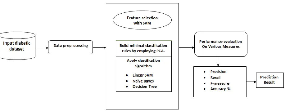
Figure 1. Proposed Model diagram A. Principal Component Analysis (PCA)

PCA is a mathematical method used for data analysis. It is one of the most significant features extraction techniques, the major use of principal components analysis is to Reduce the feature and to handle missing values. The principal component analysis is a dimensionality reduction method that is usually used to reduce a large number of input variables to a small number of variables that still contains most of the information as a large dataset [17].

Mathematical proof of principal component analysis: Let‟s assume we have two predictors. Which are X and Y. we have two observations for each. X = {1,2}, Y = {2,1}. First, we will make this data into a standardized form, i.e., Mean of X = 1.5, Mean of Y = 1.5.

Standardized X =

X-mean (x) Y-mean (Y)

-0.5 0.5

0.5 -0.5

Covariance (X,Y) = 1( ( ) ( ( ))

1

n

i X mean X Y mean Y

n



   



Normally, PCA transforms a set of dependent variables into a set of independents which handles with uncorrelated variables called Principal Component (PC). Most of the major possible variances will be recalled in the first PC and then the next PCs will decrease the possible variances.The objectives of PCA are to reduce the dimension of the data and select new variables that relevant to the best outcome. Two approaches are using in PCA. i.e., Eigenvalues and Eigenvectors.

Algorithm-1: PCA Algorithm

Steps of Principal component Analysis:

Step 1 – Transforming the data to a similar scale Step 2 – Standardized the data. i.e., Re-center the original dataset to the origin at means zero

Step 3 – Calculate eigenvalue and eigenvector of the covariance matrix.

Step 4 – Calculate trace and variance explained by principal components.

Step 5 – Derive the new data through the selected principal components. (New = eigenvector * Data).

Brief description of the PCA in the diabetic dataset, features range is very high (1 to 100) and some features range is very low (0 to 1) due to which high features have more effect on the predictions of output as compared to the low features data. Find the covariance of data to find the correlations between all features. After that find the Eigenvalues and eigenvectors of the covariance matrix. Next, sort the eigenvectors by decreasing eigenvalues and choose k eigenvectors with the largest eigenvalues. Use this eigenvectors matrix to transform the samples onto the new subspace.

(4)

IV. CLASSIFICATION ALGORITHMS A. Linear SVM

A linear support vector machine or linear SVM is probably the best linear classifier out there. SVM (Support Vector Machine) is a supervised learning algorithm which is mainly used to classify data into different classes. Unlike most algorithms, SVM makes use of a hyperplane which acts as a decision boundary between the various classes. SVM is a set of related supervised learning method used in medical diagnosis for classification and regression. A linear SVM is no different from other linear classifiers except for the fact that it attempts to find a hyperplane with the largest margin that splits the input space into two regions. It gives the best generalization capabilities due to the larger margin.

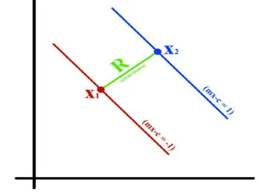
[image:4.612.90.275.324.463.2]

SVM can be used to generate multiple separating hyperplanes such that the data is divided into segments and each segment contains only one kind of data. Support Vector Machines classification algorithm Consider two hyperplanes:

Figure 2. Distance between two Hyper planes R is the perpendicular distance between two hyperplanes which is called Margin of both the hyperplanes. And this margin is computed as

2

1 *

m

X

R

m





henceforth, Briefly, SVM works

by identifying the optimal decision boundary that separates data points from different groups (or classes), and then predicts the class of new observations based on this separation boundary.

B. Decision Tree

A decision tree is a type of supervised learning algorithm (pre-defined target variable) that is mostly used in classification problems. In the decision tree, we split the population or sample into two or more homogeneous sets (or sub-populations) based on most significant splitter/differentiator in input variables.

How does the Decision Tree algorithm work? All decision tree algorithms have the same structure. Basically, it's a greedy divide-and-conquer algorithm.

1. Take the entire data set as input.

2. Search for a split that maximizes the "separation" of the classes. A split is any test that divides the data in two (e.g. if attribute 5 < 10).

3. Apply the split to the input data (the "divide" step) into two parts.

4. Re-apply steps 1 and 2 to each side of the split (the recursive "conquer" step).

5. Stop when you meet some stopping criteria.

6. (Optional) Clean up the tree in case you went too far doing splits (called "pruning")

The evaluated performance of Decision Tree technique using Confusion Matrix is as follows:

decision tree algorithm uses information gain.

2 1

inf( )

m

log

i

D

 



_

pi

where, Pi is the probability that an arbitrary tuple in D belongs to class Ci.

1

inf ( )

A v_j

(

)

Dj

D

X Info Dj

D



 



( )

inf( ) inf ( )

_A

Gain A



D



D

where, Info(D) is the average amount of information needed to identify the class label of a tuple in D. |Dj|/|D| acts as the weight of the jth partition.

InfoA(D) is the expected information required to classify a tuple from D based on the partitioning by A. Attribute A with the highest information gain, Gain(A), is chosen as the splitting attribute at node N().

2 1

inf ( )

log

v

j

Dj

Solit

o D

D







 





_



_







Where,

|Dj|/|D| acts as the weight of the jth partition. v is the number of discrete values in attribute A.

The gain ratio can be defined as

( )

inf ( )

Gain A

Gainrati A

Solit

o D



The attribute with the highest gain ratio is chosen as the splitting attribute

C. Naïve Bayes classifier

(5)

probability that a given tuple belongs to a particular class. This classification is named after Thomas Bayes (1702-1761) who proposed the Bayes theorem.

Bayesian formula can be written as: P(H | E) = [P(E | H) * P(H)] / P(E)

The basic idea of Naïve Bayes‟ rule is that the outcome of a hypothesis or an event (H) can be predicted based on some evidence (E) that can be observed from the Bayes‟ rule.[16] This algorithm provides a prediction model in relation to the likelihood of certain outcomes. Naive Bayes algorithm measures patterns or relationships among data by counting the number of observations. The algorithm then creates a model that reflects the patterns and their relationships. After creating this model, it can be used as a prediction of several objectives.

V. RESEARCH METHOD

This research is an experiment on PIDD-Pima Indians Diabetes Dataset [18] on the original dataset and PCA based reduced dataset Calculation of each classifier is in terms of a number of rules obtained and classification accuracy with 10-fold cross-validation. Anaconda 3.7 with Spider 3.5 framework coding in Python.

A. Data Description

our methodology evaluated on PIDD-Pima Indians Diabetes Dataset, which is taken from UCI Repository. The dataset includes data from 768 women with 8 characteristics, in particular:

Table 1. Attribute description

S.No Attribute Abbreviation of

Attributes 1 Number of times pregnant preg

2 Plasma glucose

concentration

pl

3 Diastolic blood pressure (mm Hg)

pr

4 Triceps skinfold thickness sk 5 2-Hour serum insulin (mu

U/ml)

in

6 Body mass index (weight in kg/(height in m)^2)

ma

7 Diabetes pedigree function pe

8 Age (years) ag

9 Class „0‟ or „1‟ cl

The last column of the dataset indicates if the person has been diagnosed with diabetes (1) or not (0).

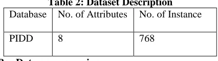
[image:5.612.319.532.76.136.2]

where the value of one class '0' treated as tested negative for diabetes and value of another class '1' is treated as tested positive for diabetes. Dataset description is defined by Table-1 and the Table-2 represents Attributes descriptions.

Table 2: Dataset Description Database No. of Attributes No. of Instance

PIDD 8 768

B. Data preprocessing

Data preprocessing is an initial phase to accomplish the task on raw data which applies data normalization and split up incomplete data, outlier‟s data and inconsistent data before the data is used to other procedures. PCA is a procedure to transform the data dimension and find a new set of variables by selecting the subset of the principal component without losing the important feature. The best significant subset evaluation has been collected and used in the next step for the experiment.

C. Classification Algorithms

The classification phase learns the data set from the previous step by using three classification algorithms i.e. Decision Tree, linear Support vector machine and Naive Bayes algorithms.

D. Performance Evaluation Statistical Measures

For the calculation of the section of the predicted positive cases, the below-mentioned formulas are used. Precision P using TP is True Positive Rate and FP is False Positive Rate and they defined as,

Pr

ecision P

TP

TP FP





(1)

The proportion of positive cases that were correctly identified are known as True Positive Rate (TPR). It is calculated as

Recall

TP

TP FN





(2)

Where FN = False Negative Rate In this research work, there are three measures used. Correctly classified instances are properly classified by any classification technique. Accuracy is calculated by an exact value.

TP +TN

Accuracy

TP+ TN+ FP+ FN



(3)

The mentioned rule for the accuracy calculation the above-mentioned formula is used with TN = True Negative.

Sensitivity =

TP

TP+ FN

(4)

TN

Specificity

TN+ FP

(6)

The F-Measure can be computed as some average of the information retrieval precision and recall metrics.

2Recall Precision

F

Precision + Recall

[image:6.612.83.287.109.226.2]



(6)

Table 3. Confusion Matrix [15] Predicated

Positive

Predicated Negative

Actual Positive TP FP

Actual Negative FN TN

VI. EXPERIMENTAL RESULTS

[image:6.612.318.536.303.434.2]

Between three classification algorithms. For this implementation, 8 features from the data set are used. Table 4. shows comparative performance of classification algorithms with different parameters such as Precision, Recall, F-measure and accuracy. From the above table, it validates that the accuracy of the Decision tree is 75%, likewise, Naïve Bayes classifiers got the accuracy of 76% and Support vector machine got the accuracy of 68% respectively.

Table 4. Comparative Performance of Classification Algorithms on Various Measures.

Table 5. The Performance Classification Without PCA

Classifiers Decision Tree

Naive Bayes

SVM

Correctly

classified 576 583 522

Incorrectly

classified 192 185 246

Accuracy 75% 76% 68%

Table 5 shows the classification's accuracy of rule-based system in diabetic data set without applying PCA between three classification algorithms. For this implementation, 8 features from the data set are used. The results show that Naive Bayes classifier can classify 76 % correctly while decision Tree classifier performed 75% and support vector machine 68% respectively.

Table 6.The Performance Classification With PCA Classifiers Decision

Tree

Naive Bayes

SVM

Correctly classified

585 594 527

Incorrectly classified

183 174 241

Accuracy 76.22% 77.36% 68.68%

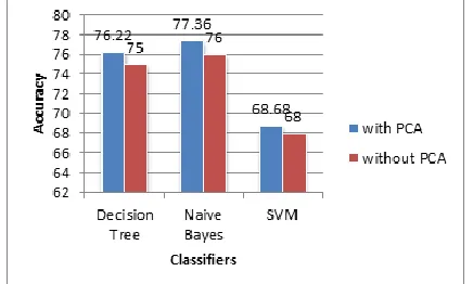
[image:6.612.77.291.384.608.2]

Table 6 indicates the results of three classifiers with PCA. From the data set, there are only 7 features used for classification. It shows that Naive Bayes classifier proved to be the most accurate classifier for the accuracy of 77.36% by 1.36 % increased. In addition, decision tree and SVM classifiers got an improvement of 1.22 % and 0.68 %, respectively.

Fig. 3. Comparison performance of three classifiers with and without PCA

The bar chart gives information about the comparison of the rule-based system of three proposed classifiers with and without PCA approaches as shown in Figure 3. According to the chart, the number of rules is decreased in the case of the classifiers with PCA. It shows that Naive Bayes classifier proved to be the most accurate classifier for the accuracy of 77.36% by 1.36 % increased. In addition, decision tree and SVM classifiers got an improvement of 1.22 % and 0.68 %, respectively.

VII. CONCLUSION

[image:6.612.79.294.388.501.2]

(7)

Bayes and SVM classifier. It found that naïve Bayes classifier giving the best accuracy of 77.36% respectively.

REFERENCES

1. Komi, M., Li, J., Zhai, Y., & Zhang, X. (2017, June). Application of data mining methods in diabetes prediction. In Image, Vision and Computing (ICIVC), 2017 2nd International Conference on (pp. 1006-1010). IEEE.

2. Kavakiotis, I., Tsave, O., Salifoglou, A., Maglaveras, N., Vlahavas, I., & Chouvarda, I. (2017). Machine learning and data mining methods in diabetes research. Computational and structural biotechnology journal.

3. Nilashi, M., bin Ibrahim, O., Ahmadi, H., & Shahmoradi, L. (2017). An Analytical Method for Diseases Prediction Using Machine Learning Techniques. Computers & Chemical Engineering.

4. Mercaldo, F., Nardone, V., & Santone, A. (2017). Diabetes Mellitus Affected Patients Classification and Diagnosis through Machine Learning Techniques. Procedia Computer Science, 112(C), 2519-2528.

5. Kandhasamy, J. P., & Balamurali, S. (2015). Performance analysis of classifier models to predict diabetes mellitus. Procedia Computer Science, 47, 45-51.

6. Perveen, S., Shahbaz, M., Guergachi, A., & Keshavjee, K. (2016). Performance analysis of data mining classification techniques to predict diabetes. Procedia Computer Science, 82, 115-121.

7. Orabi,K.M.,Kamal,Y.M.,Rabah,T.M.,2016.EarlyPredictiveSyst emforDiabetesMellitusDisease,in:IndustrialConferenceonData Mining,Springer.Springer.pp.420–427.

8. Esposito, F., Malerba, D., Semeraro, G., Kay, J., 1997. A comparative analysis of methods for pruning decision trees. IEEE Transactions on Pattern Analysis and Machine Intelligence 19, 476–491. doi:10.1109/34.589207.

9. Priyam,A.,Gupta,R.,Rathee,A.,Srivastava,S.,2013.Comparative AnalysisofDecisionTreeClassificationAlgorithms.InternationalJ ournalofCurrentEngineeringandTechnologyVol.3,334– 337.doi:JUNE2013,arXiv:ISSN2277-4106.

10. Saravananathan, K., & Velmurugan, T. (2016). Analyzing Diabetic Data using Classification Algorithms in Data Mining. Indian Journal of Science and Technology, 9(43).

11. Pradhan,P.M.A.,Bamnote,G.R.,Tribhuvan,V.,Jadhav,K.,Chabu kswar,V.,Dhobale,V.,2012.AGeneticProgrammingApproachfor DetectionofDiabetes.InternationalJournalOfComputationalEngi neeringResearch2,91–94.

12. A.Rashid,S.M.A.,Abdullah,R.M.,Abstract,2016.AnIntelligentA pproachforDiabetesClassification,PredictionandDescription.Ad vancesinIntelligentSystemsandComputing424,323–

335.doi:10.1007/978-3-319-28031-8.

13. Han, J., Rodriguez, J.C., Beheshti, M., 2008. Discovering decision tree based diabetes prediction model, in: International Conference on Advanced Software Engineering and Its Applications, Springer. pp. 99–109.

14. Sharief,A.A.,Sheta,A.,2014. Developing a Mathematical Model to Detect Diabetes Using Multigene Genetic Programming. International Journal of Advanced Research in Artificial Intelligence (IJARAI) 3, 54–59. Doi:10.14569/IJARAI.2014.031007.

15. Nai-Arun,N.,Moungmai,R.,2015.Comparison of Classifiers for the Risk of Diabetes Prediction. Procedia Computer Science 69,132–142. doi:10.1016/j.procs.2015.10.014.

16. Sunita Joshi, Bhuwaneshwari Pandey, Nitin Joshi, “Comparative analysis of Naive Bayes and J48 Classification Algorithms”, IJARCSSE, vol. 5,no .12, Dec 2015.

17. J.-W.Liu, Y.H.Chen, and C.H.Cheng, “Owa based information fusion method with PCA preprocessing for data classification,” in International Conference on Machine Learning and Cybernetics, 2012, pp. 3322– 3327.