Polynomial approach to nonlinear predictive generalized minimum variance control

Polynomial Approach to Nonlinear Predictive

Generalized Minimum Variance Control

Mike J Grimble and Pawel Majecki

Industrial Control Centre

niver-ityoI' trathclyde

Graham Hills Bui!ding

50 George Street

GLASGOW GI IQE

nited Kingdom

. elephane N": +44 (0) 141 5482378

Facsimile 0: +44 (0) 141 5484203

lectronic Mail: [email protected]

Abstnlct

A relati ely simple approach to Nonlinear Prediclive (;en 'rali:;ed Minilllum Variance (NPGMV) contr 1 is

intr' duced for nOl1lin,"()J" di"cr 'Ie-lime tIIulli Jllriuh!" systems, The system i repre ented by a comhination

of a stable nonlinear ubsystem where no tructure i assumed and a lin ar subsy tern that may be unstable

and modell d in polynomial matriA form. The multi-step predictive control cost index to b minimised

in olves both wei ht d error and control signal cosling terms. he NPCMV control law involves an

as umption on the ch icc of cost-function weights to ensure the existence of a stable n nlinear clos d-Ioop

1

controller r duces to a polyn mial matri.\ version of the well known CPC c ntroller. In the limiting case

when the plant is nonl inear and the cost-function is ingle tep the controller becomes equal to the

polynomial matrix version of the so called Nonlinear Generalised Minimum Vuriunce controller. Th

contr Iler can be implemented in a form related to a nonlinear version of the Smith Predictor but unlik thi'

compensator a stabilizing control Jaw can be obtained for open-loop unstable proc sses.

Keywords: polynomial systems. optimal, predictive. nonlinear. minimum variance, tran-port delays.

Introduction

The aim is to introduce a relatively simple controller for n nlinear systems and one that has sam of the

advantages of the popular polynomial ba ed (jenerulised Predictive Control (OPC) algorithms. It is well

known that n nlinear (NL) systems have more complex behaviour than tinear systems, including limit cycle

respon es and chaotic behaviour. The proposed controller does not rely on local linearization and it

provides a global optimal control solution.

h lin ar muriel based predictive (:ontrol (MBPC) approach ha' been appli d very suc 'essfully in

the pro ess industries, where it has improved the profitability and competitivene s of production plants. [t

has been u d to improve perfonnance in dirncult system which contain long dead times, time-varying

sy·tem parameters and Illultivariable interactions. The approach is often thought to be easy to und rstand

relati e to other modern control design methods. The predictive contrul alg rithms were tir. t applied in

low processes for the chemical, petrochemical, toad and cement industrie', but ar now used on faster

application. uch as servo, hydraulic systems and gas turbine applications. A predictive controller usc

futur r fercnce signal inlonllation and minimises a Illulti- tep co t-function. The most p pular algorithms

are DYI/amic Mutrix ('nf1tr( I (DM ) [I

J.

Generali::: 'd Predictive ('untrol (GPC) [2,3], an the algorithms

ofRichalet [4,51. The relationship bdwecn LQ optimal and predicfi\'(: "onfrol was xplored in f6].

The GPC controller was originally obtained in a polynomial sy t m form. The c ntr I strategy

bused Illultivariabl systems. The assumption was made that th plant model could be decompo ed into a

set of delay tem1 . a 'ery general nonlinear sub yst m that had t be stabl and a linear sub ystem that

could be repre ente I in polynomial matrix or state e uation form and include unstable modes. This

prabl m was analysed in r8-1 0). The maj r development over the basic GMV control law in [9J involves

an extension of th NGJvrv cost-index to in lude future tracking error and control costing terms in a GPC t pe of problem where the linear ,·ub-system of the plant model is repre ented in polynomial matrix

equation form. When the system i linear the controller is e uiv' lent to a GPC controller that is a practical solution f, r many applications.

There is of course a rich history 01' relatively recent research n nonlinear predictive c ntrol [J 1-241,

but the proposed approach i om what ditferent. since it is c10s r in spirit to that of fixed model based

design than n online optimization algorithm. An advantag of the new predictive control approach is that

the plant model can be in a very general nonlinear operator form, which might involve hard nonlinearities.

a tate-depend nt state-space model, transfer operators or ev n nonlinear function I ok up tabh::s. The plant

can includ both linear and nonlinear subsystems and no structure needs to be known for til nonlinear

block but this must be as umed open-loop stable in an appropriate sense. 0 guarantee closed loop tability

the as umplion is made that a c rtain nonlinear operator ha a stable inverse.

It i· \V 11 known f r linear system that stability for thi type of control law insured when the

c mbinati n of a control weighting function and an error weighted plant model is stricti minimum phase

125J.

For nonlinear syst m a related operator is required to have' stabl inverse. This implies that th

c t-function weighting must be chosen to sati

Iy

b th pert! rmance and stability/robustn 5S requirelll nls.

rhe plan for this paper i as fall ws. The nonlinear plant and linear di. turbam:e m dels in

p lynomial matrix torm are described in § 2. It is sho\'\'n in

S

3 that the solution or the linear multi-step

predicti

(Gro

contr I problem can be tound from the solution of an equivalent minimum variance

control problem. The cost function nd the solution of the NPGMV nonlinear optimal control problem arc described in . 4. t gether with the main theorem. A design example is presented in § 5 and finally

conclusions are ummarised in § 6.

2 System Description

The a umed mod I for the plant can be severely nonlinear and dynamic and may have a very gen ral form

but th disturbance model is cho en to c linear 0 that relatively simple results are obtain d. This is not

restrictive. since in m ny applications the model for the disturbance signal is only an LTl appr ximation.

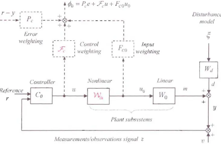
Th system shown in Fig. I includes the nonlinear ( L) plant model together ith the linear reference.

measurement noise and disturbance signal. The signals 1I(t) and

c;(t)

are vector zero-mean. independent.

white noi e signal . Th~ meu.wremenl noise signal 1 (t) is assumed to have a con tant covariance matrix

R₁

=

R~ ~

O.

There is no loss of generality in as timing that the di. 'Iurhance white n ise source ~ I) has

an identit I c variance matrix. Th re is al 0 no requirement to specifY the di tri ution of the noise s urce.

inc the structure of the system leads to a prediction equation, \.-"hieh i only dependent upon the linear

stochastic di turbance model. The plant m del can have a very general nonlinear operator form, which

might involve hard nonlinearities, a state-dependent tate- pace model, tran fer operators or ev n

nonlinear-function .look LIp tables. Detai I d knowledge of the NL system structure is not r qui red.

Nonlinear Plant: (I)

here :: -k I lIenot a diagonal matrix of the common delay element in the lit put signal paths. rhe

outputofth non-linearsLlbsystcmY\1k' that might r present actuators,wiJl bedenot d

U(I(I)=(

Iku)(t).

r

r simplicity the L subsystem: WI is a . limed to bc .finite: gain sluM!! hut the linear subsystem

W_o

=

=-k WOk • inlroduct:d b low. can contain any unstable modes. If th decompo ition into a nOI linear

and a linear sub-system is not relevant then let the linear ub-sySknl F~-;n, = I _ The g neralisatiol1 to di Ilerent delays in di rrcrent paths is . rraighUorward [26 j. The vectors f signal in the system may be

Ii t d as fall ws: 'Lio(t) E Rrr~1 (input to linear subsystem);

u.(t)

E

R'"

(control signal);

y(t)

E

R'-

(plant

output); z(t) E H'- (observations); r(t) E fl' (set-p int I reference); Yp(t) E R'" (wl.:ighted 0 tput):

2.1 Linear Sub!;y,.,tem Polynomial Matrix Models

The polynomi I matrix system models. for the incar part of the (r x In) multi varia Ie system ma now be

intr duced. The. ub-, ystems to be defin d ar associated with any lin ar sub-system W

_o

in the plant model and the linear disturbance m del. he Contmllcd AUI()-Reb71'cssive Moving Av rage (CARMA)

model, representing the linear subsystem of the plant is derin d as:

(2)

when: ';(1) and the input signal channels in the plant mod I are assum d to includ a k-sleps (k ~ 0 )

transport delay and

BfI(

Z 1)

=

B

_{Ok (Z-I)Z -k,} Th de!ayfree plant transfl r of the Iinear sub-system and the

disturbance model may therefore be defined. in tht: left coprime form:

(3)

Introduce a stable c:os/-jimc/io/1 weigh/ingmode! in left coprime form ~.(-:; 1)= ~~I(Z-ltl P_cn (;; I), he

weight d output may be written as:

(4)

The power .'pee/rUllt tor the combined di turbance and n ise il:,'T1al

I

=

II

+

'U

=

n~l~

+

/I can be

computed. noting these a 'e Iinear sub )'stcms. using cPif

=

m

_dd + (/)\T := w"W

t; + R

r ,

wh re the n tati n for

the adjoint of

WI

implies U~; (= I)

=

W:

C:-) and only in this case:: represents the ::-domain complex

number. The generali::ed s[le 'lro/~fl/etor

Y

_I may bc computed from this spectrum as Y, Y;

=

(f> /I • where

V = A-I Dr' The 5y'tem models are assumed to be such that D, is a s/riclly 8,:17/11' p Iynomial matrix

[17.18

J:

(5)

The model f r the disturbance ignal is linear. which is an as L1n1ption that does not < ffect stability

properties but may caLIs a degree of LIb-optimality inlhe di5turbanc rejection properties.

bmovations sil:lI(ll: Disturbance models are often appro.xi mated in real appl ications b. Iinear systems

driven by white noise. It is well known that the signal

I

== d + \' may be mod lied in i novations signal

form as/(t)==}jE(t), \ here

}j

=A I_Dr is defined via the spectral-factorisati n (5) and £(1) denote a

\-\·hite noise signal of zero-mean and identity covariance matrix [8,21]. The syst m description may be

as Limed to b such that Dr is strictly Schur. The ohserl'utions signa! may theref re be written. LI ing (2)

a-; z(t) == y(t) + 'u(t)

=

A-l(z-I)Bok(z-l)'Uo(l-k)

+

il1(z-I)C<J(.Z-1)';(t) +o(t)

:= A-1(z-1)Bok(z l)U(J(t - k)

+

Yj(Z-I)&(t)

(6)

Detine the right coprime model for the weighted .lpJc!ralj(.JC!or:

(7)

Then the we(Rhted observutiollS si, rna! ZT' (t)

=

P.

(z

-I ):;(1) may be wrinen a :

(8)

2.2 Optimal Linear Prediction

Th olution of the ptimal control problem require the intr duction or a least squares predictor. Thi

enables the inferred output vat times I -I-k + I . 1+ k +:?., t be caJculat d (assuming that the disturbance

at future times is null). The cost-function to be minimised, wi jch defines the [ a"t-squares predictor, is

given 'IS: ,J

=

E{.'/r,(1

+

jl/)'l (9)

where the estimation error:

(I )

and iiT,(t

+

j

I

t) derines the predicted valLIe of .1/1,(1.) at a time) steps ahead. To generate the prediction

algorithm the f !lowing iU/7hulllil1(' equarion must he 'olved for the soluljon(E). H). with E] of

First Diophalltine: ( [ I)

This equation may b written as:

D -I) J 4H ( -I)

1-

1( 1)

D (

-J)4-1(

-I) _{( 12)}

r,;.~

+

Z ) ; " " f ; ;

=

fp Z • f Z

Prediction equatioll: Substituting from (I J) the expression fI r the weighted obs rvati ns signal (8):

Zl'(t)

=

Pc

(Z-I)WOk(Z 1)/I'u(l -

k)

+

Dh)(Z-I)A_f \ : 1)1:(1)

=

~.(Z-I)~V~k(Z-I)'Uu(t - k)

+

(E}(Z-I)

+

z J-Ir:H (2 I)A/(",-I))t:(I)

ub titutin t from the innovation (6) c(t) =}'~IZ(I - D;IBok/lO(t - k) obtain:

ZI'(t)

=

~.(Z-IF~;k(Z-I)iLn(t - /,;)

+

E;(z

I)t:(t)

+

Z-7-k

H

(z

I)A;I(Z-I)(}~

I(Z-J)2(1) -

D/(z-

)BOk(z

I)no(t -

k))

J

Recall A~;t

r/

= Dr~Pc and substituting, the }I'eighled obs-rl'Oliof/s:

Weighted Output: 1'0 obtain the expression tor the weighted output

,:)f)

=

F"

z(t.)

= .

1J 1'(1)

+

11,,(1),

but from (7)

J:..

rrA( - DIi> and from (12) and ( 13):

lJp(l)

=

EJ(z

l)t.(t) -

(1,,(1)

+

Z J 4lI/z ')()'h,I(Z-I)ZI'(I.)

+(Dh,(;;-I)-Z) 4H (z 1)).1/(.::-1)1);'(.: I)ilok(z 1)'/I,\I(t-k)

J

Future Values of Weig/rled Output: Using ( 11 ). the .J + k steps ahead weighted output ign I:

(I )

To

further simplify the cqu tions (recalling

D;l

is as umed to be stable), the right coprime m del:

B1k(Z-I)D;i(z-1)

=

D/(Z-l)Bllk(Z- )

(15 )

Also let the _i!:,'Tlal 'uf(i)

=

Djl\;::;-l)ll_o(t) , then (14) may be 'ovritten:

y_r

JI

+ j + 1,;) = (E](;;-I )l:(t +) +

k) -

'l,/t +,]

+

k))

+ [

H)(Z-l)D;l(Z-1

),,)f)

+

E)(Z-1 )B1k(Z l)LLf(t

+J)]

( 16)

ote that the maxin um degree of the polynomial matrix E) i j + I,; - 1and hence the noise components in

El(t

+ ,] + /,;) includes E(

t

+ j +

1.:) "

E(

t

+

L), which ar at future times.

2.3 The Prediction Equations

The optimal predictor at time t

+ ,] +

k. gi en ob ervations up to time f, can now be derived. Consid I' first

the case wher the noise

{o(t)}

is zero. The observations. up to time { are known and the futur values of

the control inputs {'/I.o(t) ,",

"'u(t

+

j) }, us d in the predictor. are omputed at time f. and hence the future

contI' I input i independent or the future disturbance and noise sequence. It follow thal the expected

value of the "quare [.J and round (.) brack ted tCI1TI in equ tion (16) must be Lero. The predictor to

minimi e the cost (9), given thatlhe cross terms in the cost are null, follows, from (16):

( 17)

If the measurement noise ignal IS 11 n-7cro then the weighted nOI e term

"flU +.1

+

k =

P

_{ru (::;} I

U(l

+.1

+

k). If the weightingP_r.(' I) is a constant, which is usual in CPC c ntrol,

or ifit is assumed a p Iyn mial matrix of degree .I + k - J. then lJp(t + J + k) is only dependent on future \ hite m asurement nois and the expected value of such a [em and the square brack ted terms in ( 16) must

( (8)

second Diophantine eq/lalioll may nO"\1 be introduced to break up the t I'm E)(Z-l)Blk(Z-l) into a p rt

with a)+ 1 step dela. and ''I part depending on D_f1 Z 1) (recall

'U00

=

DI;(Z-I )u.[J(t)), Thus. for j 2. 0,

introduce the following Diophantine quat ion, with ( -' ' S ). of _{.1 )} smullest def,Jree forC :₎

G ( --I D (-' 1) -j-J (_-I)

=

E ( -I)B ( -J)

Second Diophantine: J ) ~ 11 '"

+ -

j ' J j ... II.: 2 ( 19)

wheredeg(G/z-I ))

=

J' The prediction. from equation (J7), may now be obtain d (for) _ ) as:

The degree of G)(z-J) is} and the secon term in (20) therefore in olves the inputs which are in th future.

Defin the signal

.t)t),

in terms of past outputs and inputs. a':

(21 )

hus, th preJided ,!'eighted nul/iul (20) may be written, for j cO. as:

(22)

Coefficient,\' (ifthe Polynomial mlltrix G_J :;-1). From equations (I 1) and (19):

'

n

P}'R )-kH lin 'J Ie

Ct J / 1 = ( ' I J I , - ' : /1 l k - Z '7,

(,' - 1) \ l

n _(- )

k H t 1H _ J 1 (.' ) 1) I

t ) - ,J Ilk '" j ·....f Ii.

+

<, v J /1

Th G)(

z

l) theretore includes the fir t J + I Marl\ov paramctcf:) 'V

J of the weighted plant C j

=

J~;~Ik'

2.4 VectorlMlitri.\: Prediction Equations

The future wight d outputs are [0 be predicted for inputs computed 111 the interval t c

[t.t

+

N]

wher N ~ O. Equation (22) may therefore be u d to obtain:

:&1'

(t

+ kit)

:Op

(t +] + kif)

gu

91 0

go 0

0 0

0

uu( t)

'uu(t + 1)

11)(1)

.I;

(t)

=

,I]J

₉₀

+ (23)

y1'(f + N +

kit)

!}N J

(IN _{gN-l !h %} v,u(t + N)

h

(I)

he ector form of the predicted weighted output:

(24)

Using (21 ). lh free respon c prt:dictions

F;.N :

So(;: -1)

H11(z-J)

taU)

IIJ(z

I)

SJ

(z 1)

AU)

Dh,l(Z 1);:;1'(1)

+

F l, _N

=

J~(t)

(25)

The functi ns [fNZ(Z-l) and SNz{Z I) are detined in an obvi us way from (25). The predicli n error

('OE(t + I,) + '"

+

'k IE(I +- I) -o,,(f + 1..)

ellf-;(f

+

1 + I;)

+ .,.

+ ('kL(t + I) - '/11'(1; +] + k)

3

Future set poillt kllowledge: The futur variations of the ref r nee si!:,'Tlal r( l) are a sumed kn wn over N

steps and the weighted rcterence 7~(t) ::: ~,(::

J)

'1'(1). The vectors ofji/ture weighted signals:

7~,

(t)

1/1' (f) Ill) (t)

T~(t+1) yp(t + 1) 'U_u

(t

+

:I)

Rt,N

=

}~,N

=

Uf~N

=

(27)

I~(t + rv) iJ

1

,(f

+

N)

uo(t

+

N)

The k steps-ahead future weighted outputs can be written in vector terms Y;+k,N

= }

~+k, +} ~+k,N and thc

fi.lture trar.;king error, that includes a dynamic error weighting, may therefore be written

a :

(28)

.

­

fhe vect r of predicted si nals }~+kN in (28) and the prediction error :r:,N are ortho onal.

Main Features of Generalised Predictive Control

reviewofth derivation of the

Gre

controller is provid d below where the input will be taken to be that

fi r the linear sub-sy tern _{(lIo )'} since it provides e ults that ar n eded for the d finition orth NL pr blem of interest. The GPC /7er.!rwmUJlce index, t be rninimi cd:

N

J :::

E{I

'1'(1 +.J + k)"'('p(l

+.i

+ k)

+A;U'o(t

+

J)'l'u

lI(l

+

j))j/} (29)

} II

wh re

J{ .It}

d 'note the conditional expectation. <.:Onditioncd on measurements lip to time I: A) den tes

n scalar control signal v eightin r and the vector of future weighle I error sign I ville

Pl,(t + j

+

k)

=

Pc (z 1)('1(1

+

j + k) -!J(t

+

J + k)) . he future optimal control is to bi: cal ulated for

the interval T € [I. t

+

N]

and til\;

cpe

,'()s/:1ill1ctiol1:

(30)

IntroJucing the optimal predictor. using (28) and (30), obtain,

where the c t weightings on the future inputs ₁₁₀ are written A ~ == diag{J,~

,1l,2 ....,

2,~}.

3.1 GPC Optimal COlltrol Solulio"

The tems in the performance criterion can be sim lified by noting the prediction errors in ~+k,N depends

on futur values or the sigr al E(

t).

wh ich ar' as umed to be indep ndent of future controls. The e timate

Y~+kN is therefore orth gonal to the estimation rror ~~k.Nand R,+J..I' is assumed 0 be a known over the

1) step. The cost may therefore be btained as:

(32)

-,

­

where

J

_o

=

E{Y,+J...\ }~+k II} is independent of the control action. 'ub tituting (24) into (32) btain:

Thu , defin (33)

and

(34 )

To minimise this conditional cost term the gradient of the cost l11U t be set to zero to obtain the vector of

futur contr Is. Note the J I tem1 is indepcnd nl of the control action and a perturbation and gradient

calculation may be appli d [27] to obtain the vector of CiPCluflire optima! controls as:

( 5)

3.2 Equivaleflt GPC Cost Minimisatiofl Problem

The above is equivalent to a s ciaI cost minimisation problem hich is needed to motivate the NPGAJIV

problem introduced later. Let the can tant matrix X _N

=

G~CN

+

A~ be factorised as:

} -r}? _=-\N \"

₌

GTG

_{TN TN}

₊

A2 (36) C'mnpletillR the squares in (34) the cost:

Th cost-function: (37)

-T 7 . U

where ¢11k.N =

Y

G, (Rt+k,N - F;,N) - Y[ t,N ( 8)

he terms that re independent of the control acti n may be written a .flO (t)

=

J{)

+

.II (I) where

(3 )

The last lenn

J\U(t)

in equation (37) doe not depend upon control action and the optimal control i found

by setting the first term to LCro, giving the same control a in (35). Thence, the GPC contr ller for th

above linear sy (em i the same a<; the controller to minimise thl: norm ohhe signal <J)W•• N in (38).

3.3 Modified Co:-.,/-I"t1ex

The abo e discussion motivates the definition of a n w fIlu!ti-sle/? minimum variance' cosl pr blem thaI has

the same olution lor the optimal controller. Can ider a new signal to be minimised of the torm:

(40)

The vector of future val lies of this signal,

()

(41 )

I '

P,.,

= G~ and (42)

The reason fi r this choice of cost terms becomes apparent below. D fine a MV Jnlllri-step cost-function as:

(43)

Predicting forward k-steps:

(44)

ow consider the signal ¢ t+k N and substitute for i :+k,N = }';.t k,lV

+

}~+k,N' Then from (44) obtain:

(45)

This expression may b written in terms of an estimate and slimation ~rrorvector as:

A _

¢I.,-I..\ =<1)1 I. \ + ¢ I ' k l (46)

The estimated prediction

ef>'+k

N

=

~'N

(RI+k,N -

}~+k,N)

+

F;~{jt~N

and prediction error:

(47)

Multi-Step Cost Jndex: The performance index (43) may therefore be simplified as:

The terms in (43) can be simplified, recalling the optimal c timate }~'k,N and the estimation error }~'k,N

are orthogonal and th~ future reference Rlflr .\ is a "nown signal. Expanding:

(48)

Thence, the cst-function: (49)

The part of the cost term independent oj'L'onlrol action may be written as:

(50)

Now simplify the vect r¢"k,N by substituting for }~+kN from (24) and using (42) and (36) obtain:

(I:> - n

(D

-

}7 )

pO

TTil -!)

R

- P (

()

F) pO

[T u

(51 )

From a similar argument the multi-step predictive control sets the squared term iT (49) to zero cD _t+

k,...

=

0,

Clearl th resulting optimal contr I [fuN _{t , ' o '}

=

)1.'~,Ip,...(R kN - F' N) is the same as the vector of future

...,lv t .... I t\

GPC control in (35).

Theorem 3.1: Equivalent Minimum Variance Predictive Control Problem

onsider the minimisation of the CPC co t index (_9) for the system and assumption introduced in ~2,

where the nonlin ar subsyst

111 V\.{k

= [

and the vector of optimal GPC controls is given by (35).

- T

Redefine the cost-index to have a multi-step variance form (43)

.l(t)

=

E{<1>t+k,..._<P,+k,N

It},

wh re

vector of future optimal controls is identical to the GPC contr Is deftn din (35).

Proof: ollow by collecting together the ab ve result.

•

4 PGMV Optimal Control Problem

The Nonlinear Pr·dictive Generalised Minimum Variance (I PGMV) contr I pr blem of interest is now

considered. The actual input to the sy tern is ofcour e the contr I signal u(l), shown in Fig. I. rather than the input to the linear sub-sy tern /1

0 ' Tht: co t-functi n for the nonlinear control problem must il1l:ludl: a

c ntr I ignal costing term, although the c sting 011 the intermediate signal ₁₁₀ (1) can be retained t

examine limiting case. This ignal may al 0 represent an Glc/l/t.l{or output that may be costed in orne

probkm. If the. mallest delay in each output channel of the plant is or magnitude k -steps this implies

that th contr I signal t alTects the output at least k -steps later. ror this rca on the control signal costing

should be d lined to have [he torm:

(52)

Typic !ly this weighting on the nonlinear sub-systen input will be a lineuI" dynamic operator but it may

also b chosen to be nonlinear to introduce an anti-windup capability [10]. This perator.r;k can be

assumed to be Cull rank and inver1ible. rhus, consider a new signal whose variance is t e minimised,

IIlV Iving the weighted sum aCerraI', subsystem input and control signals:

(53 )

In analogy with th GPe problem a multi-step ost index may be defined that is an exten i n of (43):

Extellded Multi-Step Perfurmallce illdex:

J

p

=

E {

cD:1:k,N <!>~...k.N

It}

(54)

he signal <l>~+kN i therefore extended to include the additional future comrol signal co ting term:

The non-lin ar function ~k,NUf./i will normally b defined to have the simple diagonal operator form:

(56)

where [, ;~N

=

(Y1{k,.\U

f

J

and )/l1k,x aloha a block diagonal matrix form:

Remark\':

rh

pI' blel11 implifics when N = (j to the single-step non predictive control problem, which is

the am as the so-called NGMV l;ontr I problem [9J.

4.1 The NPGMV Control Solution

The olution

r

!lows from very similar step' to those in §3.3 and wililheret'ore be summarised only briefly

and the estimatii.,l11 err 1':

- (I - · · 1 ' .'/ ­

~u

y

Th future predicted values in the signal ~1.k.N involves the estimated vector of weighted outputs l.k,N

and th se are orthogonal to }~~k ,\. AI 0 note that the estimation 1'1'01' is zero mean and hence the expect d

value orthe product with an known signal i null. The cost-functi n ma th refore be written as:

(60)

, 0

wh re the optimal ontrol ets Cl>t+k,,\

=

O. The condition/or optimality therefore has the torm,

(61 )

4.2 The Nonlinear Predictive GMV Control Signal

The future optimal control, to minimize (60), toll ws from th condition for optimality in (6J

u

_I,N

= -

( f -

_rk,J A~]/v_{N Ik,:"}

)-1

P _"N

(R

_l+k,N

-

Y )

_t+k,N

(62)

An alternative sol ution of (61), in an ea ier form for implemcn ation, gi ves:

U

=

_,T-I

(p

(R -

Y )-

A 2)1,:' ,[1 ) ₍₆₃₎

I,N ck, f"V l+k,N l+k,N N Ik,.' I,N

The optimal predictive control law is nonlinear. since it in olves the nonlinear control signal costin J term:

7;;k,N and the nonlinear model for the plant )1.{k,:-.' Furthl:r implitication is possible by sub tituting i'om

(24) tOl' the estimate

Y;

tk,N ' so that the condition lor optimality in (61) may be written as:

• ubstituting Irom (42) the condition for optimality bl:comes:

P (R -F

)+(F

-}'l'}'J'V)U

= ()

(64)

(.w t+k,N !,N k,N Ik,N t.'

The two a[ternati e solutions for the vector O//iltlll' optimal controls, n ting (36), therefore becomes:

(05 )

or

u

=

-.T I

(p

R

- F ) -

x

w

,U )

(66)

/,.. c:k,N c., l+k,N t,N N lk,:\ t .•

Remarks: The NPGMV control law in equation (65) is model based and includes an internal model for the

nonlinear process, The control la"" is to be implemented u ing a receding horizon philosophy and from the

precedin", discu si n it becomes identical to the GPC controller (35) in the limiting linear ca e when the contr I co ting tends to zero

(;z:;;

'.N ~ 0, Hik,=,

=

I), The problem construction nables an important property to be predicted and confirmed from (65), That is, if the control weighting .T.k.N~O then [Tt,N

should introduce the inverse of the plant m del Y1{k,:-: (if one exists) and the resulting veet r of future

c ntrols t~N will tl en be the same as the GPC controls for the resulting linear system,

Theorem 4.1: onlinear Predictive GMV Optimal Control Law

Consider the syst m described in §2 and th predictive control probl III for the cost index (54) (N)O),

The nonlinear plant operator V\{~ is assum d to be/illile Rain 'tabLe. For closed-lop stability the operator

(..J;;1I}(1)

=

(;Z:;:kll)( I -

k) .

dynamic error

PJ."

-I) and input

{Au, ..

AN}

COSI

wei rhtings. The muLti-step

predictive controL cost-function to be minimi cd, inv Ives a sum of future eost terms

.II'

=

E

{<t>~,rk, <t>~I'k,N

It}.

where <1>~+k.N includes the vector of fUlure error, input and contr I l:Osti ng terms:

""II P L' FI! () (·r U )

... / ...k,

= (.

D tfk "

+

(w I,h

+

.r

Ck , !oN (67)

and in terms

or

the weightin 'S ~, == G~ and 1';[~ = -A" . The NPUA'!Voptimal control law to minimize

the variance of signal (67) is given as:

[ _I." ==-(.T _ck.J -XH:'tp(R _{N lk,:- ,', t, k,1} - F ) _t,N (68)

u

_£,J\

=

-.T'!

_ck,N

(p

_('N (R _lJ-k.,N - F ) -_f,N

x

_tV

w

_lk,;\ .U ) _t. (69)

and th current control may be found from the lirst element of the vector (invoking the receding horizon

Solutio": The proof of the NPGMV ptimal control follows by collecting the results in the above section.

The necessary condition for stability an be established using the sam argument as afta the main theorem

in [9]. This r quires the introduction of some lin ar or rL plant sub-system models. Write the lin ar plant

in the right coprime torm W_o

=

B_o,4Ql and the orresponding block structure as W_o,\' = B_O,,\ ~\ Also

write the plant model In a polynomial NL operator form: so that

following relati nship may be established:

which may be liS d to h w that the model for the predicted outputs involves nly table operat rs. _

Remarks: he tw c>..pressions for the NPGMV control signal (68) and (69) lead to the two alt rnative

structure, ,hown in ·igs. 2 and 3, respectively The econd. shown in Fig. 3 how how the current and

future c ntr Is may be separated from the full vector of" future controls, a exrlaincd below. If th rror

and input cost-function weightings are defined in thc

ope

motiva! J form ~,\

=

G,(

and f~(~

=

-A;

then

tor u lincar ystem (

V\1k

= / ) the optimal control. when.r: ~0, is identical to a

ope

control law.

4.3 Implementation ofthe Predictive Optimal Control

A Llseful partition may be intr duced ",hich later enilhl(' the algorithm t be simplified. Tile co trol at time

I is computed tor N> 0 from the vector of CUITent and futur c ntrol by introducing the matrix:

('/II ==[1.0

)J

(70)

This enabl s th control at time I to be found from the ector of curr nt and future control as:

Current cOlltrol: u(l)=

[f.O... O]U

_tv (7 J)

To compute the vector of future c ntr Is for t > () al 0 introduce: (72)

Future cOlltrols:

_U

_{{N == COl} U == [ 0 (73)

ote from (70), because of the block diagonal structure f th control signal costing .!L;;k,N ' then

(74)

Th optimaL control at time t can then be computed, LI ing 69) as:

"/1.(1) =

-.T

_ck

Ie

(p

R - F ) -

x

w

u )

(75)

{(J eN t ~k,N I,N N Ik,:\' t ..'

The ve '(01' ojfiftllrL' conlrnls, computed at time t, may also be found as:

[If _t,N

==-c

_Of

;r-I

_ck,N

(p

_I" (R _{t Ik,N} -F )-X _{t,N N} )1/ _lk,J l! ) _t,N (70)

wher~ from (72) writ (' ~r I -

[0

I

J;c,

I -

[0

.T. I ]

II/"/";I<,S - I,\'JII'/II/11 \ o.,\' - 1\'1)-/11/11 ,J,. \-1 .

The vector J1{k,:Jlt ,N may be written, frOIll equation (57) (partitioning current and future tenns) a :

(77)

Using a related partition, writ ~ the matrix XiV in the (oml X \ == yl Y == r>'~ Y2]' when;

Y;

has m_u

quation for implementing the optimal control (69). may bl.: split into the curn:nt and future ontrols a

4.4

Marine Predictive Control Design Example

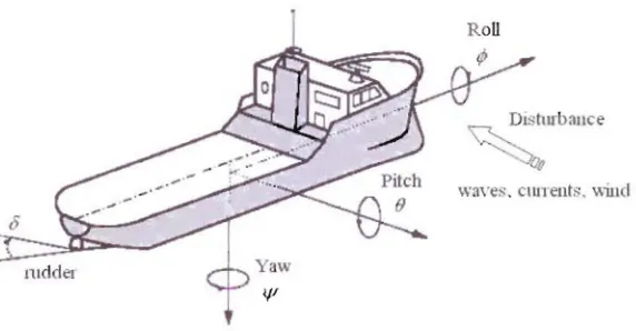
Consider the problem of the simultaneous control of the roll and yaw motions of a ship. A supply vess

with Ih onventional angle notation is shown in Fig. 5. rhe ship heading (yaw angle) is controlled b the

rudder, and it is assumed that the heading traje tory to follow is kn wn. The rolling motion cau ed by the

I' rce of the sea wave disturbances can he counteracted by the use of tin roll stabiliz rs. How ver, this

LInd sira Ie movement mey also be reduced by aclive use of th rudder, and a number of commercial

rudder roll stabilization systems have been developed ( ee [28] and referen es therein). This tr tegy

requires high-perfomlan e rudder machinery but can provide improved performance or enable smaller fins

to be used. The basic dynamics of the ship roll and yaw motion with re pect to the fin and rudder, for

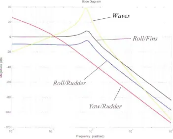
particular ship peed and encounter angle, are sh wn 'n Fiuure 6.

( .) = (0.8):'

Roll model: Ct/J .\ , 1

.1'- + 2·0.2·0.8.1' + (08)"

0.2

Yaw model: (j ( . 1 ' ) = - - ­ 'I' s(t Os + I)

( '. ) O. I(I - 4.1')

Rudder to roll illteractioll: ',;,; (,\ - - - ' - - - " " ; ' , (6s + I)

The model includes non-minimum phase interaction from the rudder to roll motion and there is an

integrator in the yaw model. he roll characteri tics of the ship are 111 d lied using are onant econd-order

ystem, with a natural frequency of 0.8 rad/sec and a 10\\ damping factor. The frequency resp nses of the

In de Is are shown in Fig. 7. he fin and r Idder actuators GI'l and G,i have hard constrail t on the

achieva Ie angle and ,'ate. The actuator limits are set as 25 eg and 10 dcg/sec for the fins, and 30 deg and

7 degisec for the rudder servo. respecti v Iy.

Di.<.tmbance!i: The effect of thl: wave disturbanc on the roll and yaw motion is rellrcsented in Fig. 13 by

_ 5s c

the signal d~ and d~,. wh re ( ¢ I - 1 1 dPJI

=

a.5 r:: and sand r" are whit n ise r +2·a.l·O.7s+(O.7t s

sequ nces. The model for th roll wave di turbance provides a second order linear approximati n to the

Pierson-Moskowi/:: spectrum, and the aw di turbance is assumed to be of low-frequency nature and is

modelled by an integrator driven by white noise.

Control objectives: Th main control objectiv s are the reduction of roll mati n and tracking of the

heading et-point. he former can be characteriLed by the Roll Reduc/ion Ra/io (RRR) defined as:

(78)

This ratio represent the improvement in roll reduction achi ed by usin feedback ontrol, with 100%

carr sp nding to the ideal null roll motion. The yaw tracking performance can be measured using

can entional measures such as rise time / settling time, or. alternatively, by integral squar error (IS£). In a classical control scheme. rolling mati n is regulat d using fin tabilizers, and the heading is controlled" ith

the ru der, involving two 5150 y terns. A multivariable control scheme will take the system interactions

into ac aunt. 'l!lowing the rudder to actively attenuate the roll and to control yaw, which is possible due to

the separation in th roll and yaw motion frequency c ntent.

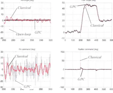
Results: For the purpose of control I r design, the continuous-time models of the system were di cretized

u ing the sample time of 0.5 seconds. In the simulations. the ship yaw angle was r quired to follow a

kn wn trajectory co isting of two step chang s, while minimizing the roll motion, accor ing to the

.p cified crit rion. In the limiting cas when

n

_1k

=

1 (i.e. no constraints in the ship mod ) and .T:k ~ 0,

the NPGMV c ntroller collapse to a version

or

the standard (fPC controller but with weighted output and

rfernee .ignals in the cost criterion. Th reults for the norninl settinTs

or

N=O,

An = 3 x diag{l 0';.5 x 10 '} and the linear case arc shown in rig. 8. The P, weighting was chosen based on a multi-loop eta sical controller (st,;e r9j), the performance ofwhi h is also hown.

The GPe results for the roll atlenuation in this uncon train d case are somewhat unrealistic and detuning the controller (increasing /L weighting) is normally needed in th pre ence of fin and rudder

constr ints (in particular. fin rate limits are exceeded). he pr dictive action can also b utilized wh n the

5

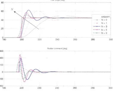
the time scale magnified to show the predictive action more clearly). Increasing values of N are indicated

by the arrow. A long prediction h rizon often leads to a faster response and also improves the robustnes of

the olution (as m asured by tl re ponse overshool), which is illustrated by the yaw angle respon' .

When th constraints are present, the GPe controller n cds to b detuned to maintain tability. he nonlinearities can be acc unted for more effectivel by introducing the nonlinear control weighting

f;.

into the NPGMV control structure. For example. defining this weighting appropriately leads to an anti­ windup structure for contr Ilers that include integral action [10]. After tunin ,the results are sh wn in fig.

10 (for N = 5), wher the NPGMV atistie the rudder angle limits that are much exce d d by the GPC design. The roll reduction is also more effecti e with the nonlinear control (about 40% improvement in

Roll Reduction Ratio) since the servo nonlineariti s ar explicitl accounted for in the contr Iler tructur .

Concluding Remarks

There are many nonlinear predictive control strategies based on slale c/'pendenl models, lineariz tion

around a trajectory and others. The aim was to try to produce a c ntrol law which is simple to implement

and thl..: result i an algorithm which Joser to traditional model based desians than to current nonlin ar

pr dictive c ntrol strat gies. The NL Predicti\"" Generalised Minimum Variunce (NPGAIV) control

problem involves a multi-st p predictive control cost-function and the introduction

or

future set-point

information. The predictive controls strateby is a development fthe NGMV _{d si b}'l1 method which is easy

to design 'lI1d implement.

It has the nie rrop~11y that if the system is linear the control reverts to thl..: GPC design method

'v hich is well known in industr. That is, th N['(jfl(' control de ign method reduces to that of (IP .

control desi:Tn when th weight

J;;k

tt:nds to zero and th system is linear ()/J J.. = I). This sugge ts a 2

ta re design process mi:=.hL b~ used wh rc the tir t stage is for a free choice CC;PC weightings ba ed upon

the linear sub-syst m~. Tl l: engineer only need considl:r the sclccti n of desirable weightings. which satisfy

suitable pert! rmance rcquirclI1l.:nts tor' the mulfiv::lriable system The NL system characteristic:; c n thell be

c nsidered in the second stage of the desi!:,'l1 wher the contr I signal co ting (.T_k possibly nonlin ar) is sel cted and stability i sues are c n idered.

If the cost horizon becomes only a single tep th n the control law revert to th s called NGMV

solution. A m thad is available for generating cost weightings that will provide a starting point for design

f9] and guarantee a stabilising initial solution. This may be a useful tarting point and the number or steps

in the pr dictive control horizon can then be increa ed which normally improve robustness at the expense

of additional computations. Clearly if thi: response are not improving by using further steps there is no

need to incr ase the computations. The control law includes an internal m del but man. f the

computations. as in traditional polynomial e uation based predictive control, simply involve the solution of

Diophantine equations and matrix multiplications.

Acknowledgements: We ar grateful for the support orthe EP RC on the Platform Grant P/C526422/1.

References

[1.1. Culler C.R. and Ramaker B.L., 1979, Dynamic matrix cuntrol - /1 computer control algorithm,

, ,I.C.H. E, 86th National Meetino, April 1979.

f2]. Clarke, D. W., C. Mohtadi and P.S. ruff.c;. 1987, Generalized prediL·tive control - Par' I. The basic

alRorithm, Part 2. E.~Ylensions ami interpretation, !\utomatica, 23. 2, pp.137-148.

[3]. Clarke. D. W., and C. Mo tadi. 1989. Prort.!rties ojgenerali. eJ predictive conlml, !\utomatica, Vol.

., 5, o. 6, pp. f{:S9-87

f4J. Richak:t J.• A. Raull. J.I.. eslud and J. Paron 1978, Model prediclive heuristic cuntrol applicQti 17.1

to indll. '{rial processes, !\lIlomatica. 14. pp, 413-428.

151.

Richalet, J., 1993. indus/rial appli '01 iOl1s of mtiJt:l hosed prediC{fv' eon{r I. AutomaticH, Vol. 29.

o. 8, pp. 1251-1274.

[61· Bitmcad R.. M Gcvers. and V. Wert7~ 1990. Adaptil'l! Oplimal Control The Thinkilll{ Um\' GPc.

[7]. Kwon W.ll. and Pearson, A. Eo, 1977. A modified quadratic' cost problem ondfeedback stahili:ation

ala linear\ystem. iEEE Transacti ns on Automati Control. Vol. AC-22. No.5. pp. 838-842.

l8]. Grimble. M J. 200 . GMV (:ol1lrol of nonlinear mullivariahle .~ys/r::m,\',UKACC Conference Con/rol

200./. Univer ity of Bath, 6-9 Sept mber.

19]. Grimble, M J. 2005, Non-linear generalised minimllm variance feedback. feedjonrard and trucking

control. Aut matica. Vol. 41. pp 957-96 .

[101. Grimble, M J. and P Majecki, 2005. Nonlinear Generalised Minimum Variance Conlrol Under

Actllu/or Saturation. WAC World Congres , Prague. Friday 8 Jul ,2005.

[11]. Cannon. M. and B. Kouvaritakis, 2001, Open-loop and closed-loop optimality in int rpolation MPC,

in onIinear Predictive Contro!' Theon! and Pracli ·e. pp. 131-/49. I E, London.

[12J. annan. M. and B. Kouvaritakis, 2002. Efficient constrain d model predictive control with

as mptotic optimality, Siam J 'ontrol Optimisation. 41 (1), pp. 60-82.

[13] Cannon, M and B. Kouvaritakis, Y.1. Lee and A.C. Broor s. 2001, Efficient nonlinear predictive

contr I, Int-rt1ationaIJ Control, 74(4). pp.361-372.

114J.

Cannon, M and V. Deshmukh and B. Kouvarital-..is. 2003. onlinear model predictive control with

polytopic in ariant sets. Alit matico 39(8). pp. 1487-1494.

r

15]. K thaI' . M. V. V. Balakrishnan and M. Morari. 1996, R bust constrained model predictive control

using Iinear matrix inequal it ies, .!/ulOlnatic:a 32( 10). pp. 1361 -1379.

116J. Michalska. H. and

D.O.

May!~, 11)93, Robust receding horizon cantI'l ofconstrained non-linear

syst'ms. 1l!.EE Trans(/( 'tiuns on AIItol1lotit' Cuntrol, 38. pp. 1623-1633.

[17]. hamma.1.. and M. Athan , 1990. Analy is of gain scheduled control for non-linear plants. /F.EE Transactions on AII/ull/utic Control. 35. pp. 898-907.

ft

81

KOLivaritaki, B.. M. Cannon and .LA. Rossiter. 1999, onlinear m del based predictive control. In!.

.J. Control. 72( 10). pp. 919-918.

1191. Lee. Y.I., B. K uv ritakis and M. C~llnon, 2003, on trained receding horizoll predictive contI' I for

nonlinear yst ms, 1111tol/la/ica. 38( 12), pp. 2093-2 I02

[20]. Mayne, D.Q.. J.B. Rawlings. C.V. Rao an P.O.M. Sc kaert, 2000, onstrained model predictive

control: stability and optimality. Automatica 36(6). pp. 789-814.

(21]. cokaert. P.O.M .. D.Q. Mayne and lB. Ra lings. J999. Suboptimal model predictive control

(feasibility implies stability). IEEE Transactions on utmnutic 'on/rol, 44(3). pp. 648-654.

[221- Brooms. A.C. and B. Kou aritakis. 2000. Succes ive constrained optimisation and interpolation in

non-lin ar mod 1based predictive control, Int. .J Control, 73(4). pp. 312- 16.

[23]. Aligower. F.. and R. Findei-en, 1998. on-linear predictive control fa distillation column.

International .~:vmposium011 NOI/-linear Mociel Predictive Control. Ascona, Switz rland.

[24]. Camacho, E.F.. 1993. onstrained gen ralized predicti e control. IEEE Transaction on Automatic

Con/rol. 38. pp. 327-332.

[25]. Grimble, M J. 2 06, Robust indus/rial cO/ltrol, John Wiley. Chichester.

[26]. Grimble. M J. 200 I, Industrial control systems desif:,Tf7. John Wiley. Chichester,

[27]. Grimble M.J. and Johnson, M.A, 1988. Optimal c ntrol and stochastic estimation. Vols. [ and II.

John Wiley, Chichester.

• rPo _I = ~,e

+

.7;u + ~'ol/o

r -.J' :- - - -:

+

I _Disturbance

- - -

-~:

Pc

:- - -

-~~

__ - - - -:

model

---

_I

+

_I

Lrror I I

---!--- __ -1-_­

weighting

: : Control : Inpw

: . ; : ; : \I' ighting

Fe

'0 : 11'eighling

'-_-&- __ 1 ,

I ..

I I

I COl1lroller

t

I Nonlinear Linear

d I In I + r + y PI lilt suh, I'stems

+

[image:27.612.112.478.115.354.2]

+ Afeasurements!ohservations signal z _'I'

Fig.l: PGMV 2-Degrees of Freedom Feedback ontrol System for onlinear Plant

Con/roller sllh.~\'s/em ,\ol1finear Ois/lirhulICI'

FlIIlIre fJ/alll

(}WpUl

refireI/o'.,

SOl/hI/ear (lfII!r(l{or ill""r e

+

Ohsen'(uio/ll' z

+

"

Fig. 2: First Form of the NPGMV Polynomial Controller Structure

[image:27.612.101.499.425.562.2]

('ontroller Structure I'll/lire cOlI/rals

XU/Sf!

( •f

r

ulllre l.

~l!!.N

reference

t­

+

IlIplll

,l1eGsliremellls ar ab. ervatians

Plant

Disturbance

z

Fig. 3: econd Form of NPGMV Controller (sholl'ingjilfure control siRnal generalion)

Roll

wa\·e~.Clurent;;. willd

[image:28.612.100.515.115.279.2] [image:28.612.165.451.372.521.2]

d¢

0

G

a

a

'"

G¢;

¢;

,<:?\.

-~ '<;Y

- ,<y

Fins Roll rn del

_--.

Co

I - - ­

,....

f - - ­

Rudder to roll

GorP

interaction

Controller

;; _lJI-tO\

5, _to\

,.-+

G

_r5

GIJI

_~'<Y

'<;Y

fIIr d~1

Rudder Yaw model

Fig. 6: Block Diagram of the Ship Model

Bode Dagram 40

Yaw/Rudder

·20 iii ~

..

"C ₀₄₀

€ _c

'" '" :; -60 ·80 100

Roll/Rudder

_____ Waves

\ . _ - - - - Roll/Fins

120

10 < 10'

Frequency (rad/sec)

10 o

I· ig. 7: Frequency Rcspon ·cs of the System Model and Wave Spectra

[image:29.612.126.477.387.668.2]

Roll angle (degj Yaw angle ldegJ

~--30 50 ­

GPC

20 Classical 40

10' 30

0 20

Classical

10 ·10 '

-20 ~

_GPC

0

Open-loop

-30 -10

200 220 240 260 280 300 0 100 200 300 400 500 600

F"., cornmnd [degJ Rudder corrrrand [degl

30 100

Classical _Classical

20

..---­

50

0

""'"

-7

-50

_GPC

-20

-30

GPC

-100

200 220 2~u <.uv 280 300 0 100 200 300 400 500 600

Fig. 8: Comparison Nominal

erc

and Classical Cootrol Results (N= 0)

I

10

[image:30.612.120.496.125.434.2]

Yaw angle (deg!

,...

80

N 60 ~

setpoint,

N=O N = 1 - N = 3 40

20 _{--.-- N = 5}

_. __ .• N

=

9

0

180 200 220 240 260 280 300

Rudder corrmand [degl

_ .

300

.,

200;

100

0

-100

-200

180 200 220 240 260 280 300

Fig. 9: NPGMV Results - Effect of Varying the Prediction Horizon (N= 0, 1,3,5.9)

[image:31.612.122.502.127.436.2]

Open-loop Roll angle [oog]

50

::r-\

40

10 30

0 20

I

-10 10

-20 0

GPC

-10-­

-30

-0

0 IUU 200 300 400 500 600 0 100 200 300 400 500 600

Fin COfl'Yl"\3 nd Idegj Rudder cOfl'Yl"\3nd !clegj

100 400

-GPC

50

200

0 Wi

-50

7

'~CPC

-100 ·200

NPGJvfV

-150 -400

0 100 200 300 400 500 600 0 100 200 300 400 500 600

[image:32.612.105.510.121.431.2]