Automatic speaker segmentation using multiple features and distance measures: a comparison of three approaches

City, University of London Institutional Repository

Citation

:

Kotti, M., Martins, L. P. M., Benetos, E., Cardoso, J. S. and Kotropoulos, C.

(2006). Automatic speaker segmentation using multiple features and distance measures: a

comparison of three approaches. Paper presented at the IEEE International Conference on

Multimedia and Expo (ICME 2006), 9 - 12 July 2006, Toronto, Canada.

This is the unspecified version of the paper.

This version of the publication may differ from the final published

version.

Permanent repository link:

http://openaccess.city.ac.uk/2105/

Link to published version

:

http://dx.doi.org/10.1109/ICME.2006.262727

Copyright and reuse:

City Research Online aims to make research

outputs of City, University of London available to a wider audience.

Copyright and Moral Rights remain with the author(s) and/or copyright

holders. URLs from City Research Online may be freely distributed and

linked to.

City Research Online:

http://openaccess.city.ac.uk/

[email protected]

AUTOMATIC SPEAKER SEGMENTATION USING MULTIPLE FEATURES AND DISTANCE

MEASURES: A COMPARISON OF THREE APPROACHES

Margarita Kotti1, Lu´ıs Gustavo P. M. Martins2, Emmanouil Benetos1,

1_{Department of Informatics, Aristotle Univ. of Thessaloniki}

Box 451, Thessaloniki 541 24, Greece

E-mail: {mkotti,empeneto,costas}@zeus.csd.auth.gr

Jaime S. Cardoso2, Constantine Kotropoulos1∗

2_{INESC Porto, Porto}

Portugal

E-mail:{lmartins,jsc}@inescporto.pt

ABSTRACT

This paper addresses the problem of unsupervised speaker change detection. Three systems based on the Bayesian Information Crite-rion (BIC) are tested. The first system investigates the AudioSpec-trumCentroid and the AudioWaveformEnvelope features, implem-ents a dynamic thresholding followed by a fusion scheme, and fi-nally applies BIC. The second method is a real-time one that uses a metric-based approach employing the line spectral pairs and the BIC to validate a potential speaker change point. The third method consists of three modules. In the first module, a measure based on second-order statistics is used; in the second module, the Euclidean distance andT2Hotelling statistic are applied; and in the third mod-ule, the BIC is utilized. The experiments are carried out on a dataset created by concatenating speakers from the TIMIT database, that is referred to as the TIMIT data set. A comparison between the perfor-mance of the three systems is made based ont-statistics.

1. INTRODUCTION

Automatic speech segmentation aims at finding the speaker change points in an audio stream. It is a preprocessing task for audio index-ing, speaker identification - verification - trackindex-ing, automatic tran-scription, information extraction, topic detection, speech summa-rization and retrieval.

Among the most popular techniques for speaker segmentation are these based on the Bayesian Information Criterion (BIC) [1, 2, 3, 6, 7, 9]. However, BIC-based speaker segmentation is time consum-ing, a fact that has motivated research towards alleviating its compu-tational demands [8]. Tritschler and Gopinnath used the BIC on the mel-cepstrum coefficients (MFCCs) [3]. Delacourt and Wellekens proposed a two-pass segmentation technique called DISTBIC that improved the performance by utilizing distance-based segmentation before applying the BIC. [1]. Ajmera et al. introduced a BIC alterna-tive, which does not need tuning [2]. Meanwhile, novel features like the smoothed zero crossing rate (SZCR), the perceptual minimum variance distortionless response, and the filterbank log coefficients were introduced by Huang and Hansen [8]. METRIC-SEQDAC is another method [7]. Finally, a hybrid algorithm, which combines metric-based segmentation with the BIC and model-based segmen-tation with Hidden Markov Models (HMMs) is proposed [6].

The major contribution of this paper is in the comparative per-formance of three speaker segmentation systems. All systems are based on the BIC and their efficiency is tested on the TIMIT dataset using the same experimental protocol. Moreover, their performance is further assessed by usingt-statistics. The first system investigates

∗_{This work has been supported by the FP6 European Union Network of}

Excellence MUSCLE ”Multimedia Understanding through Semantics, Com-putation and Learning” (FP6-507752).

scalar and vector features as described in Section 2, an adaptive dynamic thresholding for the scalar features, and a fusion scheme which combines the partial results so as to achieve a better perfor-mance than that obtained without fusion. The second system is an improved real-time speaker change detection system able to recog-nize speaker turn points with the shortest possible delay, without having access to the entire speech stream. This scenario imposes cer-tain limitations on the computational load of the algorithm [4, 5]. In this system, the processing has two main stages: In the first stage, a metric-based approach is implemented using the Line Spectral Pairs (LSP). In the second stage, the BIC is used to validate the poten-tial speaker change points detected previously. In the third novel system, there are three modules: In the first module, scalar features and a second-order statistical measure is implemented. In the second module, the MFCCs and the delta MFCCs are used in conjunction with theT2 Hotelling statistic and the Euclidean distance. Finally, in the last module the MFCCs and the delta MFCCs are utilized, but the decisions are taken with respect to the BIC.

The rest of the paper is organized as follows. In Section 2, the three systems are described. Experimental results are shown in Sec-tion 3 and conclusions are drawn in SecSec-tion 4.

2. THREE SYSTEMS FOR SPEAKER CHANGE DETECTION

2.1. The first system

The system relies on the BIC variant proposed in [2]. The selection of the appropriate features is of great importance, since the accurate representation of the audio signal is vital. We utilize the MFCCs, the maximum magnitude of the DFT coefficients in a speech frame, the short-time energy (STE), the AudioSpectrumCentroid, and the Au-dioWaveformEnvelope. Multiple passes are allowed. In the first four passes, we use the MFCCs; in the fifth pass the maximum DFT mag-nitude; in the sixth pass the STE; in the seventh pass the MFCCs; in the eighth pass the AudioSpectrumCentroid; in the ninth pass the maximum DFT magnitude, and in the last pass the AudioWavefor-mEnvelope. Multiple passes are employed because after each pass, the number of chunks is decreased, due to specific potential change points are discarded being false. Several researchers have come to the conclusion that the larger the chunks are, the better the perfor-mance is, because there is enough data for satisfactory parameter estimation of the speaker model [1, 3, 4, 5, 8]. The decisions taken in one pass are fed to the next pass as in a Bayesian network.

The dynamic thresholding refers only to scalar features such as: the maximum magnitude of DFT, the STE and the AudioWavfor-mEnvelope. We start with an ad hoc thresholdϑthat is determined after a considerable number of experiments during which we com-pute theF₁measure, as defined in (15), for several threshold values and then we retain the value which maximizes theF1measure. Let us consider a recording that hasIchunks andI−1possible speaker change points. The value ofI is determined at the previous pass. We test the possible speaker change pointcj which lays between chunkskandk+ 1. Iff(k)is the current feature value computed at chunkk, we estimatef(k)andf(k+ 1)and then we calculate the value of the absolute difference between these values denoted by

=|f(k+ 1)−f(k)|. Let¯be the mean value ofover all chunks of a recording:¯=_I−1₁I_l=1−1|f(l+1)−f(l)|.Then¯is compared toϑ, whose value is adjusted as follows:

ϑ=

ϑ+ 0.005¯ whenϑ <¯

ϑ−0.005¯ whenϑ >¯. (1) Whenever a feature vector is employed (such as the MFCCs and the AudioSpectrumCentroid) the BIC is used. To estimate the GMM needed in the BIC, the EM algorithm is used. The EM algorithm may converge at local minima. There is no guarantee that a local mini-mum coincides with the global minimini-mum or that there is only one local minimum. This issue, combined with the fact that the BIC is a weak classifier leads us to propose a fusion scheme. Thus, we could theoretically reduce the error introduced by the EM algorithm by re-peating the experiment multiple times, sayRtimes, and applying a majority voting. To be more specific, for each repetition we obtain a set of possible speaker turn points. The set of change points after all repetition in this pass consists of those potential speaker change points that make their appearance at a sufficient frequencyS. Both

RandS are determined heuristically. Typical values forRandS

are 5 and 4, respectively. The just described procedure is detailed in [9].

2.2. The second system

This system is an improved version of the real-time speaker change detection system described in [9]. The second system starts by down-sampling the input speech audio to 8 kHz, 16 bits mono channel format and applying pre-emphasis. The speech stream is then di-vided into analysis frames of 25ms duration without overlap. From each frame 10-order LSPs features are extracted [9]. In contrast to the system described in [9], where only the voiced speech frames determined by a voiced/unvoiced/silence classifier were processed, the current system processes all the available frames. Although one would expect the system performance to deteriorate by omitted the voiced/unvoiced/silence classifier, the experimental results demon-strate the opposite. Such findings may be attributed to the limited success of the aforementioned classifier to determine accurately the voiced frames.

In the first stage, speaker change detection is coarsely performed using a metric-based approach to calculate the distance between con-secutive and non-overlapping speech segments. Each speech seg-ment includes 55 speech frames corresponding to 1.375 sec. As-suming that the LSPs are Gaussian distributed, each speech segment can be modelled by a multivariate Gaussian. It has been found by experiments that the aforementioned number of frames is the mini-mum number of frames that prevents an ill-conditioned covariance matrix for 10th -order LSPs. The Kullback-Leibler (K-L) divergence shape distance [12] is used to estimate the distance between two

sub-sequent speech segmentsiandj:

D(i, j) =1

2tr[(Σi−Σj)(Σ

−1

j −Σ−i1)] (2) wheretrstands for the trace operator.

Letfndenote the 10th-order LSP feature vector extracted from thenth frame. The covariance matrixΣiof theith segment is:

Σi=

cov{f₁₊₂₇₍i−1

2 ), . . . ,f55+27(i−21)} wheniis odd cov{f₅₆₊₂₇₍i

2−1), . . . ,f110+27(i2−1)} wheniis even

(3) wherecovstands for the covariance matrix operator. Using (2), a potential speaker turn point can be detected between two segments, whenever the following conditions are satisfied:

D(i, i+ 1)> D(i+ 2, i+ 3) (4)

D(i, i+ 1)> D(i−2, i−1) (5)

D(i, i+ 1)> ϑi. (6) The first two conditions guarantee that a local maximum exists. The third condition assures that the local maximum is a prominent one. However, it is based on a thresholdϑi, whose value cannot be se-lected trivially. An automatic threshold selection, which is based on the values of the distances between the pastN consecutive speech segments, is proposed in [4]:

ϑi = α

N

N

n=1

D(i−2n, i+ 1−2n) (7)

whereαis a scaling factor used to tune the system response. The best system performance is obtained forα=0.8 whenN=3.

To reduce the false alarm rate, the BIC is used in the second stage to validate any potential speaker change point detected by the coarse segmentation procedure. LetN(µi,Σi)andN(µj,Σj)be the Gaussian models derived from two speech segments andNiand

Njbe the corresponding number of feature vectors used in the esti-mation. Let alsoN(µ,Σ)be a single Gaussian model estimated on the union of the aforementioned speech segments, the BIC difference between the two models can be defined as:

BIC(Σi,Σj) =1

2

(Ni+Nj) log|Σ| −Nilog|Σi|

−Njlog|Σj|−1

2λ(δ+ 1

2δ(δ+1)) log(Ni+Nj) (8)

whereλ is the penalty factor for the model complexity, here set equal to 0.6, andδis the feature vector dimension (i.e. δ = 10). IfBIC(Σi,Σj) takes a positive value, the two speech segments are likely to originate from different speakers, so the speaker change point is accepted. Otherwise, the two segments correspond to the same speaker and no speaker change point is declared.

To implement a continuous updating of the speaker model, we make use of a solution based on quasi-GMM modelling, a non-iterative technique that allows real-time operation with a reasonable accuracy [4]. Instead of considering one audio segment modelled byN(µi,Σi), a speaker model is used which is approximated by a quasi-GMMN(µqGMM,ΣqGMM). This speaker model is com-posed ofSGaussian mixturesN(µm,Σm),m= 1,2, . . . , Sover

updating the current quasi-GMM speaker model. This allows bet-ter statistical independence between the models under comparison as required by the BIC. Let alsoN(µj,Σj), withj = i+ 1be the Gaussian density of the speech segment located just after the po-tential speaker change point under validation. The distance between the density modelsN(µqGMM,ΣqGMM)andN(µj,Σj)can be roughly estimated as:

BIC(ΣqGMM,Σj) =

S

m=1

wmBIC(Σm,Σj) (9)

wherewm = Nm

N_qGMM and NqGMM =

S

m=1Nm. Whenever

BIC(ΣqGMM,Σj) >0, the potential speaker change previously detected by the metric-based approach is confirmed as an actual speaker boundary by the BIC refinement procedure.

2.3. The third system

The third system is a novel one that consumes less time than the first system, because it avoids the multiple iterations. It resembles the second system. To be more specific, it consists of three modules. In the first module, the best 5 scalar features among 24 features are derived and a second-order statistical measure is employed. In the second module, the MFCCs are utilized in conjunction with the Eu-clidean distance and theT2Hotelling statistic. In the third module, MFCCs and delta MFCCs are used in combination with the BIC.

In the first module, we investigate a total set of 24 features. The set includes the mean and the variance of the following feature values, their first-order (delta) and second-order (delta-delta) differ-ences: magnitude of the DFT, STE, AudioWaveformEnvelope, and the maximum of AudioSpectrumCentroid. A feature selection algo-rithm is applied in order to derive the optimum feature subset for classification. In particular, we select the best 5 out of the 24 fea-tures. The search strategy implemented is Branch and Bound. The criterion utilized for selection is based on the maximization of the ratio of the trace of the inter class scatter matrix over the trace of the intra class scatter matrix [11]. Starting from the most effective fea-ture, the 5 best selected features are: the mean magnitude of the DFT, the delta AudioWaveformEnvelope, the mean STE, the AudioWave-formEnvelope, and finally the variance of the delta magnitude of the DFT.

Next, we consider each feature among the 5 best sequentially. Each audio recording is segmented to windows with duration of 2 sec and the feature values are computed for 2 adjacent windows. Each window is divided into acoustic vectors of 0.040 sec duration with overlap of 0.020 sec. For every acoustic vector we compute a scalar feature. For the first window, the sequence of feature val-ues has a covariance matrix denoted byX. LetYbe the covari-ance matrix of the sequence of feature values for the second win-dow. The statistical measure proposed is a second-order statistical measure value is computed for this window pair. It is a combination of the arithmetic meana(X,Y), the geometric meang(X,Y), and the harmonic meanh(X,Y)of the eigenvalues ofYX−1 defined as follows:

a(X,Y) =tr(YX

−1₎

δ , g(X,Y) =

det(Y) det(X)

1

δ

h(X,Y) = δ

tr(XY−1) (10)

The ratiologa_g(₍X_X,_,Y_Y))has been previously used in [1, 13] and the

ra-tiologa_h(₍X_X,_,Y_Y)₎ was proposed in [13]. With the combination of these two we employelog(a(X,Y)2/g(X,Y)h(X,Y))and we expect

improved results. Moreover, symmetrization can improve the clas-sification performance, compared to both asymmetric terms taken individually [1, 13]. Symmetrization results to the proposed statistic measure:

K= log(a(X,Y)2/g(X,Y)h(X,Y))+ log(a(Y,X)2/g(Y,X)h(Y,X))

= 3 log tr(XY−1) + 3 log tr(YX−1)−6 logδ (11) whereδ=50. Next, we compareKwith an ad hoc thresholdϑ. If

K >ϑthen a turn point is assumed between the two windows, else the potential speaker change point is discarded. Then the pair of the windows is shifted by 0.5 sec. This procedure is repeated for every scalar feature so 5 different possible speaker change points sets are computed, each for every feature. These sets are fused in a parallel Bayesian Network so as to produce the final set of possible speaker change points. A parallel network was used because it outperforms a tandem network while detecting Gaussian signal in Gaussian noise [10].

In the second module, the implemented features are the MFCCs and the utilized distances are the Euclidean distance and theT2

Hotelling statistic. If the first window is modelled by the Gaussian distributionN(mX,ΣX), the second window byN(mY,ΣY)and the union of the two windows byN(mZ,ΣZ),T2Hotelling statis-tic is defined as [8]:

dT₂= NXNY

NX+NY(mX−mY) T_Σ−1

Z (mX−mY) (12) whereNX, NY is the number of frames within each window re-spectively and each frame has a duration of 40 msec. In this case, a tandem Bayesian Network is utilized, since in the two detector case the tandem network is dominant [10]. It has also been proven that it is better to place the detector with the better performance later in the chain. We experimentally found that theT2Hotelling statistic outperforms the Euclidean distance, which is rather logical, since the Euclidean distance does not take into account the correlation that might exist between the data of the first and second window by not taking into account theΣZmatrix. As a result we first examine the potential speaker change points by using the Euclidean distance and then, we re-examine them usingT2Hotelling statistic.

In the final third module, the BIC is implemented. The reason why BIC is the applied last is the fact that BIC performs better when the segments are long enough [1, 3, 4, 5]. This module has two stages. In the first stage, the BIC is computed in conjunction with the MFCCs and the potential sets of potential speaker change points are fed to the second stage , where BIC is used with delta MFCCs to produce the final set of speaker change points.

3. EXPERIMENTAL RESULTS

In order to assess the performance of the aforementioned algorithms the TIMIT dataset was created by concatenating speakers from the TIMIT database. TIMIT is an acoustic-phonetic database including 6300 sentences and 630 speakers who speak English. The audio for-mat is PCM, the audio samples are quantized in 16 bit, the recordings are single-channel, the mean duration is 3.28 sec and the standard de-viation (st. dev.) is 1.52 sec. For all three systems parameters were fine-tuned using the complete TIMIT dataset (43 speech files), not including any of the files used on the evaluation.

use the false alarm rate (F AR) and the miss detection rate (M DR) defined as:

F AR= _GTF A_{+F A} M DR= MD_GT (13) whereF Adenotes the number of false alarms, M D the number of miss detections, andGTstands for the actual number of speaker turns, i.e. the ground truth. A false alarm occurs when a speaker turn is detected although it does not exist, a miss detection MD occurs when the process does not detect an existing speaker turn. On the other hand, one may employ the precision (P RC) and recall (RCL) rates given by:

P RC=CF C_DET RCL= CF C_GT (14) whereCF C denotes the number of correctly found changes and

DET is the number of the detected speaker changes. For the lat-ter pair, another objective figure of merit is theF1measure

F₁= 2P RC RCL

P RC+RCL (15)

that admits a value between 0 and 1. The higher its value is, the better performance is obtained. Between the pairs (F AR,M DR) and (P RC,RCL) the following relationships hold:

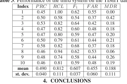
M DR= 1−RCL F AR= _{DET P RC}RCLF A_{+RCLF A}. (16) Table 1 demonstrates the performance for 10 randomly selected test recordings extracted from TIMIT database not included in the training procedure. In Table 2, the results for the same 10 ran-domly selected test recordings are demonstrated for the second sys-tem, whilst in Table 3 the corresponding results are shown for the third system. The efficiency has been presumed dropping whenever the speaker’s utterance has a duration of less than 1-2 sec, as it was expected [1, 3, 4].

Table 1. Performance of the first system on the TIMIT dataset.

Index P RC RCL F₁ F AR M DR 1 0.83 0.56 0.67 0.17 0.44 2 0.90 0.75 0.82 0.10 0.25 3 1.00 0.45 0.62 0.0 0.55 4 0.62 0.82 0.72 0.36 0.18 5 0.64 0.90 0.75 0.36 0.10 6 0.85 0.79 0.81 0.15 0.21 7 0.69 0.65 0.67 0.31 0.35 8 0.93 0.76 0.84 0.07 0.24 9 0.69 0.58 0.63 0.31 0.42 10 0.65 0.69 0.67 0.35 0.31

mean 0.780 0.700 0.720 0.218 0.305

st. dev. 0.137 0.136 0.008 0.135 0.136

Table 2. Performance of the second system on the TIMIT dataset.

Index P RC RCL F1 F AR M DR 1 0.67 0.89 0.76 0.31 0.11 2 0.60 0.90 0.72 0.38 0.10 3 0.78 0.64 0.70 0.15 0.36 4 0.78 0.78 0.78 0.18 0.22 5 0.41 0.78 0.54 0.53 0.22 6 0.61 0.85 0.71 0.35 0.15 7 0.73 0.85 0.79 0.24 0.15 8 0.72 0.76 0.74 0.23 0.24 9 0.74 0.82 0.78 0.23 0.18 10 0.78 0.74 0.76 0.17 0.26

mean 0.680 0.80 0.730 0.280 0.200

st. dev. 0.120 0.080 0.070 0.120 0.080

Table 3. Performance of the third system on the TIMIT dataset.

Index P RC RCL F₁ F AR M DR 1 0.45 1.00 0.62 0.55 0.00 2 0.50 0.58 0.54 0.37 0.42 3 0.53 0.82 0.64 0.42 0.18 4 0.47 0.82 0.60 0.48 0.18 5 0.47 0.80 0.59 0.47 0.20 6 0.50 0.79 0.61 0.44 0.21 7 0.58 0.82 0.68 0.37 0.18 8 0.46 0.94 0.62 0.53 0.06 9 0.48 0.74 0.58 0.44 0.26 10 0.46 0.81 0.59 0.48 0.19

mean 0.490 0.812 0.607 0.455 0.188

st. dev. 0.040 0.111 0.037 0.060 0.111 4. CONCLUSIONS

The performance of three BIC-based speaker segmentation systems is compared in this paper. Each system was evaluated on the TIMIT dataset. The first system puts a higher emphasis on the accuracy than the real-time operation and is the most stable of all since the standard deviation ofF₁ is 0.008. The second system favors the real-time operation. The third systems tries to compensate between the first system and the second one. The third system is also more stable than the second one since the standard deviation ofF1is approximately 50% of that of the second system.

In order to compare a pair of systems we use thet-statistics for unequal variances to test whether the difference in the meanF1 mea-sure attained by these systems is statistically significant. Comparing the first and the second system, we find that the statistic admits the value 4.48833 with a probability of accepting the null hypothesis (i.e., the two means are equal) 0.0015 that is clearly below 0.05. Accordingly, the performance difference among these two systems is statistically significant for 0.05 level of significance. Similarly, when comparing the second and the third systems as well as the first and third systems the performance differences are found to be statis-tically significant for 0.05 level of significance.

5. REFERENCES

[1] P. Delacourt and C. J. Wellekens, “DISTBIC: A speaker-based segmentation for audio data indexing,”Speech Communication, vol. 32, pp. 111-126, September 2000.

[2] I. Ajmera, I. McCowan, and H. Bourlard, “Robust speaker change detection,”

IEEE Signal Processing Letters, vol. 11, no. 8, pp. 649-651, August 2004. [3] A. Tritschler and R. Gopinath, “Improved speaker segmentation and segments

clustering using the bayesian information criterion,” in Proc.6th European Conf. Speech Communication and Techology, pp. 679-682, September 1999. [4] L. Lu and H. Zhang, “Speaker change detection and tracking in real-time news

broadcast analysis,” in2004 IEEE Int. Conf. Acoustics, Speech, and Signal Pro-cessing, vol. 1, pp. 741-744, June 2004.

[5] T. Wu, L. Lu, K. Chen, and H. Zhang, “UBM-Based Real-Time Segmentation for Broadcasting News,” in Proc.2003 IEEE Int. Conf. Acoustics, Speech, and Signal Processing, vol. 2, pp. 193-196, April, 2003.

[6] H. Kim, D. Elter, and T. Sikora, “Hybrid Speaker-Based Segmentation System Using Model-Level Clustering,” in Proc.2005 IEEE Int. Conf. Acoustics, Speech, and Signal Processing, vol. 1, pp. 745-748, March, 2005.

[7] S. Cheng and H. Wang , “METRIC-SEQDAC: A hybrid approach for audio seg-mentation,” in Proc.6th Int. Conf. Spoken Language Processing, October 2004. [8] R. Huang and J. H. L. Hansen, “Advances in unsupervised audio segmentation for the broadcast news and ngsw corpora,” in Proc.2004 IEEE Int. Conf. Acoustics, Speech, and Signal Processing, vol. 1, pp. 741-744, May 2004.

[9] M. Kotti, E. Benetos, C. Kotropoulos, and L. G. P. M. Martins “Speaker change detection using BIC: A comparison on two datasets,” in Proc.2006 IEEE Int. Symp. Communications, Control, and Signal Processing, March 2006. [10] Y. Zhu and X. Rong, “Unified Fusion Rules for Multisensor multihypothesis

net-work decision systems,” in Proc.2003 IEEE Trans. Systems, Man, and Cyber-netics, vol. 33, no 4, pp. 502-513, July 2003.

[11] F. van der Heijden, R. P. W. Duin, D. de Ridder, and D. M. J. Tax,Classification, Parameter Estimation and State Estimation, London UK: Wiley, 2004. [12] J. P. Campbell, JR, ”Speaker recognition: A tutorial”,Proccedings of the IEEE,

vol. 85, no. 9, pp.1437-1462, 1997.