Remote Sensing Image Registration Using Multiple
Image Features
Kun Yang1,2,†, Anning Pan1,2,†, Yang Yang1,2,∗, Su Zhang1,3,∗, Sim Heng Ong4and Haolin Tang1,3
1 School of Information Science and Technology, Yunnan Normal University, Kunming 650092, China; [email protected] (K.Y.); [email protected] (A.P.); [email protected] (H.T.)
2 The Engineering Research Center of GIS Technology in Western China of Ministry of Education of China, Yunnan Normal University, Kunming 650092, China
3 Laboratory of Pattern Recognition and Artificial Intelligence, Yunnan Normal University, Kunming 650092, China
4 Department of Electrical and Computer Engineering, National University of Singapore, Singapore 117576, Singapore; [email protected] (S.O.)
* Correspondence: [email protected] (Y.Y.); [email protected] (S.Z.) † These authors contributed equally to this work.
Abstract:Remote sensing image registration plays an important role in military and civilian fields, such as natural disaster damage assessment, military damage assessment and ground targets identification, etc. However, due to the ground relief variations and imaging viewpoint changes, non-rigid geometric distortion occurs between remote sensing images with different viewpoint, which further increases the difficulty of remote sensing image registration. To address the problem, we propose a multi-viewpoint remote sensing image registration method which contains the following contributions. (i) A multiple features based finite mixture model is constructed for dealing with different types of image features. (ii) Three features are combined and substituted into the mixture model to form a feature complementation, i.e., the Euclidean distance and shape context are used to measure the similarity of geometric structure, and the SIFT (scale-invariant feature transform) distance which is endowed with the intensity information is used to measure the scale space extrema. (iii) To prevent the ill-posed problem, a geometric constraint term is introduced into the L2E-based energy function for better behaving the non-rigid transformation. We evaluated the performances of the proposed method by three series of remote sensing images obtained from the unmanned aerial vehicle (UAV) and Google Earth, and compared with five state-of-the-art methods where our method shows the best alignments in most cases.
Keywords: remote sensing; image registration; multiple image features; different viewpoint; non-rigid distortion
1. Introduction
Remote sensing image registration refers to the fundamental task in image processing to align two or more images of the same scene (i.e., the sensed images and the reference images), which can be multiview (obtained from different viewpoint), multitemporal (taken at different times) and multisource (derived from different sensors). In this paper, we mainly focus on registering the remote sensing images taken from different viewpoint. As a basic technology in the field of remote sensing image processing, it has been widely used in the field of military and civilian such as natural disaster damage assessment, resource census, assignment of climate changes, military damage assessment, environment monitoring and ground targets identification, etc.
Existing remote sensing image registration methods can be approximately classified into two categories: area-based methods and feature-based methods. Various reviews on image registration methods can be found in [1–5]. Area-based methods use the pixel intensities of identical image windows to estimate similarity while feature-based methods extract image features (e.g., points, lines,
and regions) and match them using similarity criteria [6]. When there are noises, complex distortion and significant radiometric differences between the images to be aligned, the computation complexity or the search space of the area-based methods will increase nonlinearly with the transformation complexity and feature-based methods are more robust and preferable. In this paper, the captured remote sensing images exist the local non-rigid geometric distortions caused by ground relief variations and imaging viewpoint changes, thus we mainly focus on feature-based methods for registration. Such methods generally consists of three steps [7]: (i) feature descriptors extraction; (ii) feature point sets registration; (iii) image transformation and resampling.
Generally, a good feature descriptor should be distinctive and at the same time robust to changes in viewing conditions as well as to errors of the point detector [8]. For desirable local image descriptors, to improve distinctiveness while maintaining robustness is the main concern [9]. Among the popular local invariant features which have been proposed in remote sensing image registration (e.g., Harris [10], scale-invariant feature transform (SIFT) [11–13] and speeded-up robust features (SURF) [14]), Mikolajczyk et al. [8] demonstrated that the performance of SIFT [11] under affine transformation, scale change, rotation, image blur, jpeg compression, and illumination change outperforms other local invariant descriptors in most of the tests. There are various researches for remote sensing image registration based on the variants of SIFT algorithm or the combination of SIFT and some other algorithms. Li et al. [15] proposed a new criterion named scale-orientation joint restriction criteria in order to overcome the intensity difference between remote sensing image pairs. Sedaghat et al. [16] introduced an automatic registration algorithm by extracting high-quality SIFT features in the uniform distribution of both the scale and image spaces. In addition, other variants of SIFT such as PCA-SIFT [17], SAR-SIFT [18], AB-SIFT [6] and SIFT-DRS [19] are also proposed in literatures. Furthermore, Goncalves et al. [13] developed a new AIR (Automatic image registration) method based on the combination of image segmentation and SIFT, and the method is complemented by a robust procedure of outlier removal. In [20], a novel coarse-to-fine scheme for automatic image registration based on SIFT and MI is proposed, and their method achieved the outlier removal and also can generally reject most incorrect matches.
Feature-based methods are typically formulated as a point set registration problem, since point representations are general and easy to extract. In order to achieve a robust point registration, it is crucial to construct putative correspondences based on local invariant feature similarity at first and then estimate the spatial transformation based on geometric structure feature constraint [21–23]. Here, we briefly review some point set registration methods since our method is based on feature point. Fischler et al. proposed the classical random sample consensus (RANSAC) [24] algorithm. Myronenko and Song [25] introduced a probabilistic method, called the coherent point drift (CPD) algorithm, for both rigid and non-rigid point set registration. Moreover, Liu and Yan [26] investigated how to discover common visual pattern discovery via spatially coherent correspondences and recover the correct correspondences. Zhang et al. [27] defined the spatially consistent topic model by making full use of the correlation between image classification and annotation. Recently, Ma et al. proposed a robustL2-minimizing estimate (L2E) [28] for non-rigid point set registration, they later proposed a flexible and general algorithm called locally linear transforming (LLT) [29] for both rigid and non-rigid registration on remote sensing images. More recently, Yang et al. [30] proposed a new method named GLMDTPS, which considers global and local structural differences as a linear assignment problem.
viewpoints since the images usually contain local non-rigid distortion. (iii) It is ill-posed for mapping one feature point set to another by a non-rigid transformation model since the solution is not unique.
In this paper, we present a new method for remote sensing image registration with different viewpoints. Compared with the current methods, the major differences and advantages of this paper are as follows. (i) Probabilistic model construction: the mixture-feature Gaussian mixture model (MGMM) is constructed for simultaneously dealing with different types of image features. (ii) Feature complementation: Making the respective advantages of Geometric structure and intensity information to complement each other, i.e., the Euclidean distance and shape context to measure the similarity of global and local geometric structure discrepancies, and the SIFT distance to measure the scale space extrema, both of which are combined and substituted into the mixture model by which the reliable correspondence is obtained. (iii) Geometric constraint: a regularization term to prevent the ill-posed problem based on coherent velocity field is introduced into the L2E-based energy function for better behaving the non-rigid transformation.
The rest of this paper is organized as follows. Section2introduces our method in detail. Section3 demonstrates the registration performance of our method on various types of remote sensing images with different viewpoints against other methods, followed by some concluding remarks in Section4.
2. Methodology
We first introduce the three major contributions of the proposed method: (i) modeling of the MGMM; (ii) feature specification and combination; and (iii) geometric constrained energy function. Whereafter the main process is demonstrated, followed by the method analysis.
2.1. Mixture-Feature Gaussian Mixture Model (MGMM)
The motivation behind the development of MGMM is the need for estimating reliable correspondence using multiple image features whereas the Gaussian mixture model (GMM) can only work on single feature. In this subsection we detail the derivation of the MGMM.
Based on the reasonable assumption that points from one set are normally distributed around points belonging to the other set, we therefore consider the registration of two point sets as a GMM probability density estimation problem. Letyjbe the centroid of thejthGaussian component,xitheith
data. The probability density function (PDF) is obtained as:
p(xi) = (1−ζ) m
∑
j=1Cijp(xi|yj) +ζ1
n, (1)
wherep(xi|yj) = 1
(2πσ2)
de 2
exp
−kxi−yjk2
2σ2
with the equal isotropic covariancesσ2shared,Cij = m1
are nonnegative equal quantity with∑mj=1Cij = 1, which are called the priors of the GMMs. 1n is
an additional uniform distribution with a weighting parameterζ, 0 ≤ ζ ≤ 1 for outlier dealing. However,p(xi|yj)considers only the Euclidean distance and might lead to insufficient robustness
in some registration scenarios, e.g., although the local structure around xa and xb are different,
p(xa|yj) = p(xb|yj)ifkxa−yjk2=kxb−yjk2.
Consequently, the MGMM which is capable of dealing with multiple image features is developed. The PDF of the MGMM is formulated as:
f(xi) = (1−ζ) m
∑
j=1Mijf(xi|yj) +ζ1
n, (2)
where f(xi|yj) = 1
(2πσ2)
de 2
exp
− Gij+αLijandαis a constant.Gm×nandLm×nexploit the global
and local geometric structure discrepancies, priorsMm×nare specified by measuring the discrepancy
Once we have the PDF of the MGMM, the correspondence between the two point sets can be easily inferred through the posterior probability of the MGMM which is written as:
pij=
Mijf(xi|yj)
∑m
k=1Mikf(xi|yk) +ζ1n, (3)
wherePm×nis the posterior probability matrix by which the newly estimated coordinates ofxican be
obtained. It is worth nothing that two strategies for constrainingPare herein under consideration: (i) a single normalization enforcing∑mj=1pij =1 and (ii) a double normalization which additionally
requires∑n
i=1pij = 1. Intuitively, the former acts like an one-to-many correspondence estimation,
whereas the latter provides an one-to-one counterpart. In our method, the number of the feature points are strictly equal because the applied SIFT feature extractor. In addition the outlier to data ratios, however, are unknown and varied due to the different overlap ratios of each image pair. In this case it is inappropriate for requiring an one-to-one correspondence since the presence of outliers might trap the estimation, whereby the first strategy is chosen in this paper.
2.2. Combination and Complementation of Multiple Image Features
The distinctiveness of feature points, which affects the accuracy of the feature matching, are mainly determined by the robustness of the involved measures. However, different types of measures have their own advantages and limitations, where our idea is to make their respective advantages complementary to each other. In order to make the paper more self-contained, we succinctly discuss the concept of the three features we used, i.e., the Euclidean distance, the SC and the SIFT distance. The combination of features and the complete form of posterior probability function Equation (3) are then discussed.
2.2.1. Euclidean Distance
The squared Euclidean distance ofxiandyjis simply written as:
gij=kxi−yjk2. (4)
It acts a straightforward global estimation with insufficient robustness in many scenarios. To alleviate this problem,gijis commonly treated as an argument of a Gaussian function, which therefore
plays a flexible global estimation by the help of the changeable covariances.
2.2.2. Shape Context (SC)
(a) (b)
bT
hi
bR
(c)
bT
hj
bR
(d)
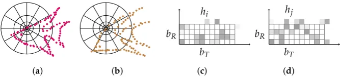
Figure 1.Illustration of the SC. (a) and (b): diagrams of log-polar histogram bins centered atxiand
yjused in computing the shape contexts. (c) and (d): each shape context e.g.,hiorhjis a log-polar
histogram of the coordinates of the rest of the point set measured using the centered point as the origin, where darker denotes larger value.
The work in [34,35] proposed the SC. A detailed illustration of the SC is shown in Figure1. The SC constructs a polar coordinate withBRbins in the radial direction andBT bins in the tangential
bin and obtains two 1×Bsets{hi(b)}Bb=1and{hj(b)}Bb=1, respectively, whereB=BR×BT. The SC discrepancy ofxiandyjis measured using Chi-square distribution as:
lij=
1 2
B
∑
b=1[hi(b)−hj(b)]2
hi(b) +hj(b)
. (5)
The SC is robust especially in scenarios like contour point set registration and hand-written characters matching, etc., because the geometric structure of these shapes are quite distinctive. However, it can also be deteriorated ifxiandyjhave similar neighborhood structure.
2.2.3. SIFT Distance
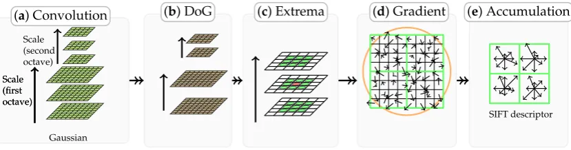
The SIFT algorithm introduced by Lowe is a classic algorithm, it first repeatedly convolves the images with Gaussians to produce the set of scale space images and obtains the difference-of-Gaussian images. The feature points are detected by comparing a pixel with its neighbors at the current and adjacent scales. Histograms of local oriented gradients around each feature points are then computed, obtaining an 128-dimensional vector as the SIFT descriptor, as shown in Figure2. Finally, a process for matching the feature points are carried out. A matching pair is detected, if its distance is closer thanτ times the distance of the second nearest neighbor. Thus, the feature points extracted from the sensed and reference images are of the same number, i.e.,|X|=|Y|, where| · |denotes the cardinality of a set, and each pair with the same suffix are matched already from the view of intensity information.
Scale (first octave)
Scale (second octave)
(a) Convolution
Scale (first octave)
Gaussian
(b) DoG (c) Extrema
SIFT descriptor (d) Gradient (e) Accumulation
Figure 2. Illustration of how the SIFT feature descriptor is obtained. (a): Repeatedly convolving initial image with Gaussians to produce the set of scale space images. (b): Subtracting adjacent Gaussian images to produce the difference-of-Gaussian images. (c): Extrema detection by comparing a pixel (marked with red circle) to its 26 neighbors in 3×3 regions at the current and adjacent scales (marked with green circles). (d): Feature descriptor creation by computing the gradient magnitude and orientation at each image sample point. a Gaussian window indicated by the overlaid circle is used as weighting. (e) Orientation histograms accumulation by summarizing the contents over 4×4 subregions (a 2×2 subregions is shown for convenience), with the length of each arrow corresponding to the sum of the gradient magnitudes near that direction within the region, generating 4×4×8 descriptors, where 8 is the number of directions.
The SIFT distance is defined as:
sij =kui−vjk2, (6)
whereSis ofm×ndimension.uiandvjare the SIFT descriptors ofxiandyj, respectively. We have
introduced three relevant features of our method, i.e.,G,LandS. The next concern is to substitute them into our MGMM.
2.2.4. Multiple Image Feature Based Correspondence Estimation
The global geometric feature discrepancy are defined byGij= gij
2σ2, whereσ
2are the covariances
the SC histograms, i.e.,Lij=lij. The Priors of the MGMMs are formulated asMij =1−esij, where
matrixSeis obtained by row-by-row rescaling which makes each entryesij∈ [0, 1], and are therefore
taken as the confidence. SubstitutingGij,LijandMijinto Equation (3), we can therefore rewrite it as:
p∗ij = (1
−esij)exp h
−gij
2σ2 +αlij i
∑m
k=1(1−esik)exp h
−gik
2σ2 +αlik i
+ (2πσ2)de2 ζ n
. (7)
The underlying assumption of density function Equation (7) is the decomposition of the process for human to recognize and categorize objects. Supposing such process is based on the linear combination among features such as Euclidean distance and density, etc. The priority of certain features may change during the process. For instance, one can easily categorize different letters according to the feature of shape at the very beginning, whereafter the accuracy can be further optimized by involving other features in. Following this idea, an deterministic annealing scheme is applied to control the fuzziness, which progressively decreases the covariances byσ2←eσ2from a large value, whereeis a constant. In the early stage of iterations, the two point sets have the biggest difference, estimation based on Euclidean distance is less accurate, yet the local geometric feature discrepancy and the intensity information are relative strong and stable. The unreliable global correspondence is filtered due to the property of negative nature exponential function. At the final stage of iterations,xi andyjare very
similar, a direct estimation using the global geometric feature is desirable. In addition, the statuses of these features interchange asσ2is small, leading to binary-like correspondences.
Furthermore, the correspondences estimation of the MGMM is a fuzzy-to-binary process, by which the correspondences are able to be improved gradually and continuously during the optimization without jumping around in the space of binary permutation matrices.
2.3. Geometric Constraint for L2E Based Energy Optimization
Based on the reliable correspondence estimated by the MGMM, the target coordinate is determined byx∗i =∑nj=1pijxj. Our next concern is to formulate a criterion, by which a reasonable positionT(yi)
ofyi is determined. This position in turn improves the accuracy of the correspondence estimation
in the next iteration interlockingly. In this subsection, we formulate the L2E based energy function with geometrical constraint. Followed by sketching out the related concepts and techniques, i.e., the L2-minimizing estimate (L2E) and the motion coherent based geometric constraint.
The unknown coordinates of the source point set to be transformed is estimated by using the L2E based energy function with geometric constraint which is written as:
Q(T,ρ2) =L2E(T,ρ2) +λ
2R(T), (8)
whereT is the non-rigid transformation,ρ2is the parameter of the density models we used to represent the deviation between the source and target point sets,L2E(·)is the L2E estimator andR(·)is the geometric constraint onT based on the Tikhonov regularization theory [36], the constantλcontrols the strength of the constraint.
2.3.1.L2E
Suppose we have a density modelp(z|θ), our goal is to minimize the estimate ofL2distance with respect toθasθ∗=arg minθR [p(z|θ)−p(z|θ0)]2dz, where the true parameterθ0is unknown. After omitting the constantR p(z|θ0)2dz, parameterθis estimated by minimizing theL2Ecriterion as:
θ∗L2E=arg min
θ "
Z
p(z|θ)2dz− 2
m
m
∑
i=1p(z|θ) #
. (9)
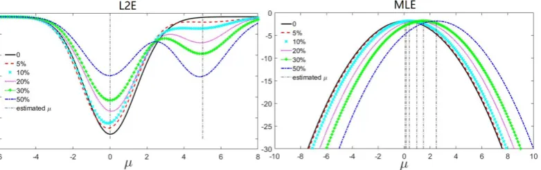
The robustness of the L2E estimator can be shown by comparing against the maximum log-likelihood estimator (MLE). Consider a sample of size 500 from a normal distributionN(0, 1) which stands for the inliers, five normal distributed samplesN(5, 1)in a tendency of increasing size (e.g., 25, 50, 100, 150, 250) act as outliers. The estimated means are shown in Figure3. L2Ehas a stable global minimum at approximately 0, as well as a local minimum at approximately 5 which becomes deeper as the number of outliers increases. This is reasonable since the outliers are from
N(5, 1). By contrast, MLE is not resistant to outliers, since the global minimum deviates more under heavier contamination.
Figure 3.The robustness comparison betweenL2EandMLE. We estimate the mean of a normally distributed sampleN(0, 1)with contaminations of extra samplesN(5, 1). The outlier to the inlier ratios are 5%, 10%, 20%, 30% and 50%. The vertical dash lines indicate the extrema.L2Ehas a global minimum at approximately 0 and a local minimum at approximately 5, both of which conform to the inlier and outlier distributions, respectively. However, the deviation of MLE increases as the ratio grows.
2.3.2. Motion Coherent Based Geometric Constraint
The key constraint of a rigid transformation is that all distances are preserved. However, once non-rigidity is allowed, there are an infinite number of ways to map one point set onto another. An appropriate constraint is necessary to solve this ill-posed problem. To this end, the motion coherent based geometric constraint is introduced into our method.
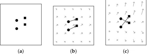
In motion perception, there are a number of important phenomena involving coherence. Velocity coherence is a particular way of imposing smoothness on the underlying transformation. The concept of motion coherence is proposed in the motion coherence theory [38] which is intuitively interpreted as that points close to one another tend to move coherently. Examples of velocity fields with two different levels of motion coherence for two different point correspondences are illustrated in Figure4. Since our focus is on its application in remote sensing image registration, we will not drill-down further into the theoretical model but directly write the geometric constraintR(T)in the form as:
R(T) =kT k2 (10)
largeλ, the constraint produces globally smooth transformation, while it produces more arbitrary transformation with small values.
(a) (b) (c)
Figure 4.Illustration of the velocity field. (a): two given point pairs. (b): a coherent velocity field. (c): a velocity field that is less coherent.
2.4. Main Process
Given a sensed image Is of size Nw× Nh and a reference image Ir of size Nw0 ×Nh0, our
goal is to obtain a transformed image It of sizeN0
w×Nh0 by recovering the underlying geometric
transformation from Is toIr. The main process of our method consists of three steps as shown in Figure5: (i) extraction of the feature point sets, (ii) registration of the extracted feature point sets, and (iii) image Transformation and resampling, where the second step comprises an alternating two-step process: correspondence estimation and transformation updating of the feature point sets.
Ir,Is
X,Y U,V
Geometric
GlobalG
LocalL
IntensityS
(a)Feature complementation
Intensity
Multiple image features Multiple image features
MGMM
Energy function ConstrainedL2E
Y← T(Y)
X∗
G,L,M
(b)Feature point set registration
TPS Bicubic interpolation
Backward approach
(c)Image transformation
ˆ Y
It
Figure 5. The summary of our method. (a): Extracting putative corresponding set{xi,yi}ni=1and SIFT descriptor set{ui,vi}ni=1using SIFT algorithm, and obtaining two types of discrepancies, i.e., the global and local geometric structure discrepanciesGandL, and intensity information discrepancyS. (b): substituting the combined features into the optimization framework and obtaining the transformed point setY, note that a loop is included. (c): Image registration based on the backward approach.ˆ
2.4.1. Extraction of the Feature Point Sets
SIFT algorithm is employed for feature point sets extraction. By {Ym×de,Vm×ds} and
{Xn×de,Un×ds}we denote the feature point sets and SIFT descriptor sets extracted from the sensed and reference images, respectively, whereY = {y1,y2, ...,ym}TandX = {x1,x2, ...,xn}T are thede
dimensional geometrical coordinates of the source and target point sets , andV={v1,v2, ...,vm}Tand
U={u1,u2, ...,un}Tare the intensity information, namely thedsdimensional SIFT descriptors forX
2.4.2. Feature Point Set Registration
Correspondence estimation:The pairwise global and local geometric structure discrepanciesG andL, and the SIFT distanceSare obtained by Equation (4)–(6), respectively. The posterior probability matrix, which is also known as the correspondence matrix is then written as:
p∗ij=
(1−esij)exp
−
kxi−yjk2
2σ2 + α
2∑Bb=1
[hi(b)−hj(b)]2 hi(b)+hj(b)
∑m
k=1(1−esik)exp h
−kxi−ykk2
2σ2 + α
2∑Bb=1
[hi(b)−hk(b)]2 hi(b)+hk(b)
i
+ (2πσ2)de2 ζ n
, (11)
whereP∗is of sizem×n. esij,esij ∈ [0, 1]is the rescaled SIFT distance,σ
2are the equal covariances
of the MGMM, constantζis the outlier weighting, andBbins are used to construct the SC log-polar coordinate. Hence, the estimated corresponding set is obtained by
X∗=P∗X. (12)
After computingX∗, the non-rigid transformation is modeled by the current correspondenceX∗ and the source point setY.
Transformation updating:The Resiz representation theorem states that ifψis a bounded linear function on a Hilbert spaceH, then there is a unique vectorνinH, makingψt=ht,νifor allψ∈ H. Thus the cumbersome mapping problem reduces to find the unique vectorν. This motivates us to model the non-rigid transformationT by requiring it to lie within the reproducing kernel Hilbert space (RKHS).
We first define a RKHSHby choosing a positive definite kernel, here we adopt the Gaussian kernel, which is in the formΘ(yi,yj) = exp(−21β2kyi−yjk2), whereβis a constant to control the spatial smoothness andΘis of size m×m. According to the representation theorem, the optimal transformation functionT takes the form
T(Y) =Y+ΘW, (13)
whereWm×de = {w1,w2, ...,wm}T is the coefficient matrix. Hence, the minimization over energy function Equation (8) boils down to finding a finite coefficients matrixW.
The non-rigid transformationT(Y)is equivalent to the initial position plus a displacement function i.e.,T(Y) =Y+V(Y). It is worth nothing thatR(T)andR(V)are exactly the same, i.e.,
R(T) =R(Y+V(Y)) =R(V), sinceR(T)is invariant under affine transformations. In this paper, we solve forVinstead ofT. The complete energy function Equation (8) takes the form as:
Q(W,ρ2) = 1 2de(πρ)de2
− 2 m n
∑
i=1 1(2πρ2)de2
exp x ∗
i −∑mj=1Θ(yi,yj)wj
2
2ρ2
+λtr(WΘW), (14)
where constantλcontrols the strength of the constraint,tr(·)denotes the trace of a matrix. Taking derivative of Equation (14) with respect to coefficient matrixW, we obtain:
∂Q ∂W =
2Θ[U(E⊗1)] mρ2(2πρ2)de2
+2λW, (15)
whereUm×de =ΘW−X ∗,E
m×1=exp{diag(UUT)/2ρ2},11×de is a row vector with all ones,diag(·)is the diagonal of a matrix, symbolsand⊗denote the Hadamard product and the Kronecker product.
by adopting another deterministic annealing on the covariancesρ2. It initializes with a large value forρ2which progressively decreases byρ2 = κρ2, whereκis a constant. And the energy function Equation (14) will converge to an optimal solution eventually.
After updating the coordinates of the source point set byY← T(Y), we anneal the covariances of the MGMM byσ2←eσ2, then return to correspondence estimation and continue the registration process until the maximum iteration number is reached. The pseudo-code of the feature point sets registration of our method is outlined in Algorithm1. In addition,
Algorithm 1:Feature matching using multiple features for remote sensing registration input :Two point setsXandY
output :Transformed point setYˆ parameter :α,ζ,β,e,λandκ
1 Initializeσ2andW;
2 Construct Gaussian kernelΘ;
3 repeat
4 Correspondence estimation:
5 ComputeG,LandSby Equation (4)–(6), respectively;
6 Compute the posterior probability matrixP∗Equation (11);
7 Compute the corresponding target point set byX∗ =P∗X;
8 end
9 Transformation estimation:
10 Initializeρ2;
11 repeat
12 Optimize the energy function Equation (14) by a numerical technique;
13 using the gradient function Equation (15);
14 Update the coefficient matrixW;
15 Annealρ2←κρ2;
16 untilreach tρiteration number;
17 Update the source point set byY← T(Y);
18 end
19 Annealσ2←eσ2;
20 untilreach tσiteration number;
21 The transformed source point setYˆ is obtained in the final iteration.
2.5. Image Transformation and Resampling
(a)MappingYˆtoYusing TPS
Estimated TPS modelP
Y Yˆ
ReferenceIr Pixel GridΓr
indexing
(b)MappingΓrusingP
GridΓs
GridΓˆr
ˆ
Γ∗=Γˆr∩ Γs
(c)Limiting indexes to boundaries (d)Getting green part fromIsasIt
based on the index
ˆ
Γ∗
It
Figure 6.Illustration of the image transformation and resampling. (a): Computing a TPS transformation modelPwhich mapsYˆ back ontoY, meanwhile, constructing a gridΓrwhich is of the same size asIr. (b): MappingΓr usingP, obtainingΓˆr. (c): Limiting indexes to boundaries ofΓˆr∩Γs. (d)
Getting intensities fromIswithin boundaries to generateIt, each pixel inItis determined by the bicubic interpolation.
LetYˆ be the source,Ythe target, the TPS kernel is defined asK(ˆyi,ˆyj) =kˆyi−ˆyjk2logkˆyi−ˆyjk,
thus, the TPS transformation model is obtained by
P= K Q QT O
!−1 Y 0 0 0 (16)
where the TPS modelPis of size(m+3)×3,Ois a 3×3 matrix of zeros andQis them×3 matrix with theithrow denotes(1,ˆyia,ˆyib), whereˆyiaand ˆyibindicate the coordinates of ˆyi.
A regular gridΓrZ×2= {γ1r,γr2, ...γrZ}T is obtained by a pixel-by-pixel indexing process on the reference imageIr, whereZ=Nw0 ×Nh0. Let gridΓrbe the source point set,Pthe TPS transformation
model, the transformed grid is obtained by first computing
ˆ
Γr Z×3=
K0 Q0P, (17)
then restoring the dimension of the grid to 2 by Γˆr ← Γˆr
(·,1) Γˆr(·,2)
, where theZ×m kernel K0 = kγri −ˆyjk2logkγri− ˆyjk,Q0is the Z×3 matrix with theithrow denotes(1,(γir)a,(γri)b)and
ˆ
Γr
(·,i)denotes theithcolumn ofΓˆr. LetΓsbe the grid obtained onIs, we have ˆ
Γ∗=Γˆr∩Γs. (18)
Finally, the transformed imageItis obtained by getting intensities from the sensed imageIsbased
onΓˆ∗, and setting the rest of pixels to black. Note that the bicubic interpolation is used to improve the smoothness ofIt, to be more precisely, the intensities of each pixel inItis determined by summing the weighted neighbor pixel intensities within a 4×4 window.
2.6. Method Analysis
probabilitiesP∗provide a badX∗, which can not leadT(Y)anymore. Moreover, we see that many green circles are missing from the red rectangle in CPD, and collapsed to(0, 0), in the contrary, all the green circles correctly distribute to where they should be, yet only the outliers have no circles in our method.
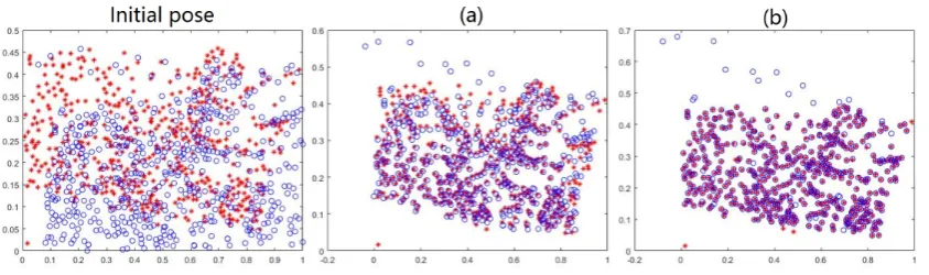
Figure 7.Demonstration of the advantage of the MGMM. Red∗: the target feature point setX. Green◦: the estimated corresponding point setX∗. Blue+: the source feature point setT(Y). Upper row and lower row: registration process of CPD and our method.XandYare extracted from a remote sensing image pair.
To examine by which the reliability of our method is mainly contributed, we also additionally compare the accuracy of the feature point sets registration using our method against GMMREG [39], which considers the registration problem as one of the aligning two Gaussian mixture models, and estimates the transformation by minimizing the L2 distance between the two models. As shown in Figure8, though the L2E estimator is employed, there exists obvious deviations in the result of GMMREG, while our method shows feasible performance. This implies that the accuracy of correspondence and transformation is mainly improved by the strategy based on the complementation and combination of multiple image features using the MGMM.
Figure 8.Examination of the availability of the MGMM. Red∗: the target feature point setX. Blue◦: the source feature point setT(Y). (a) and (b): registration result of GMMREG and our method. Obvious deviation exists in the result of GMMREG.
2.6.1. Computational Complexity
approximatelyO(m3+2m2). Overall, the time complexity of our method isO(m3). For storing kernel
Θ, the space complexity of our method isO(m2). 2.6.2. Parametric Setting
The default threshold 1.5 is used to extract the putative corresponding set{xi,yi}ni=1as well as the SIFT descriptors{ui,vi}ni=1. The bins of the SC is set to default, i.e., B = 12×5. The constant
αcontrols the trade-off between the global and local geometric feature discrepancy. The constantζ weights the uniform distribution 1n for outlier dealing. The two annealing schemes, i.e., gradually updateσ2←eσ2andρ2←κρ2, which deal with the non-convexity play important role in our method. A slow annealing, e.g., close to 1, is always preferred without the consideration of the efficiency issue. The constanttσ andtρdetermine the maximum iteration numbers of our method and the function
fminunc in Matlab.βdetermines the neighborhood size of the source point set.λcontrols the influence of the geometric constraint on the transformationT. We setα=10,ζ=0.3,e=0.9,κ=0.75,β=2 andλ=3, and initializingσ2andρ2to 1 and 0.05, respectively. Due to the iterations need termination conditions, we use the function fminunc in Matlab with the options:{MaxIter=50}, namelytρ=50,
and settσ =100.
3. Experiments and Results
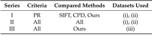
SIFT [11], SURF [14], CPD [25], GLMDTPS [30], RSOC [21], totally five state-of-the-art methods are compared against our method in the experiments. These methods can mainly categorize into three types based on the methods of feature extraction. Type 1: using open sourceVLFeattoolbox with default threshold 1.5, i.e., SIFT, CPD, GLMDTPS and ours. Type 2: using open source VLFeat toolbox with specific built-in setting, i.e., RSOC. Type 3: using Matlab open sourceOpenSURFfunction with default setting, i.e., SURF. Since both the feature matching and image registration are considered in our method, we fairly design three series of experiments. (I) Due to the employment of the same feature point sets, quantitative comparison on feature matching is carried out on methods of Type 1 using the precision ratio (PR). However, since no inlier set is outputted from GLMDTPS, the compared methods are SIFT, CPD and ours. (II) Quantitative comparison and Qualitative demonstration on image registration are carried out on all the methods using the root of mean square error (RMSE), mean absolute error (MAE) and standard deviation (SD). (III) By using the different datasets, quantitative and qualitative demonstration on feature matching and image registration are carried out to examine the availability and robustness of our method using the PR, RMSE, MAE and SD. Three datasets are used which are: (i) 100 pairs of UAV images with horizontal viewpoint changes; (ii) 150 pairs of UAV images pairs with vertical viewpoint changes; and (iii) 50 pairs of satellite images registration with horizontal and vertical viewpoint changes. The experimental design is shown in Table1. All experiments are tested on a PC with 2.20 GHz Intel CPU and 8 GB memory.
Table 1.The experimental design.
Series Criteria Compared Methods Datasets Used I PR SIFT, CPD, Ours (i), (ii)
II All All (i), (ii)
III All Ours (iii)
Table 2.Numbers of the extracted feature points.
Type 1 Type 2 Type 3 87 to 505 30 35 to 165
3.1. Evaluation Criterion
Precision [39], as well known in statistics and pattern recognition, which denotes the ability of a method matching correct SIFT feature points correspondences with low accuracy errors. The related formulations are as follows:
Precision= TP
TP+FP, (19)
whereTPdenotes true positive,FPdenotes false positive, 0≤Precision≤1. To obtain the estimated inlier setI, different approaches are used based on the characteristic of each method. For SIFT, it is just an array from 1 ton; for CPD and our method, it is obtained by:
I ={i:(PT1)i >$}, (20) where the threshold is set to$=0.75 empirically.
The RMSE, MAE and SD are used to quantify the registration accuracy. We manually determine at least 10 pairs of landmarks between the sensed image and the reference image as ground-truth, and all the landmarks are well-distributed and selected on the easily identified places around the interest areas. The related formulations and the definitions in statistics are as follows:
RMSE=
v u u
t 1
m0 m0
∑
i=1(yti−xti), (21)
The root mean square error is a frequently used measure of the distance between selected landmark and its corresponding point actually located, wherem0is the total number of the selected landmark, andytiis the landmark that corresponds toxti;
MAE=
m0
∑
i=1
|yit−xit|
m0 ; (22)
the mean absolute error is a quantity used to measure how close the landmark are to its corresponding point;
SD=
v u u
t 1
m0 m0
∑
i=1
d(xit,yti)−RMSE2
, (23)
the standard deviation informally measures how far the distance of a landmark pair are spread out from its RMSE, whered(·,·)denotes the distance.
3.2. Results on Feature Matching
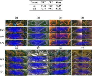
Table 3.Experimental results of series (I). Quantitative comparisons on the mean PR of Type I method are carried out. Bold fonts indicate the best results. All Units are in percentage.
Dataset SIFT CPD Ours (i) 78.30 90.81 98.25 (ii) 72.78 90.17 97.15
Figure 9.Feature matching demonstrations on eight typical image pairs of dataset (i) and (ii). Blue lines indicate true positive and true negative, red lines indicate false positive and false negative. The PRs of three methods on each image pairs are listed from (a) to (h) as follows. Ours:99.00,99.29,97.31, 97.40,99.32,99.62,98.31,98.89; SIFT: 85.68, 85.18, 45.12, 60.26, 82.43, 80.34, 82.43, 83.55; CPD: 86.86, 88.14, 85.02, 88.24, 87.22, 85.55, 89.76, 85.23.
The extraction of the SIFT feature point sets is based on the intensity information, or, to be more precisely, the scale-space extrema. However, for all the data which contain viewpoint changes, the objects captured in one image may be missing or distorted non-rigidly from another image, which further lead to false matching. Based upon the SIFT putative corresponding set, CPD estimates the correspondence using Euclidean distance, a single global geometric structure discrepancy for correspondence estimation. The motion coherent based geometric constraint is employed to regularize the displacement field between the point sets. However, as we mentioned before, the regular Gaussian mixture model is incapable of dealing with mixture features, and for Euclidean distance, p(xa|yj) = p(xb|yj)ifkxa−yjk2= kxb−yjk2even when the neighborhood structure ofxaandxb
3.3. Results on Image Registration
Quantitative comparison using the mean RMSE, MAE and SD are shown in Table 4. The transformed images and checkboards on eight typical image registration examples from dataset (i) and (ii) are shown (four examples per dataset) in Figures10and11, respectively.
A low computation complexity is one of the advantages for registering image based on the extracted feature points. However, its registration accuracy might be poor which in general cannot obtain accurate dense correspondences. Therefore, the number of the extracted feature points plays a crucial role to alleviate this problem. In this experiment, SURF and RSOC, which extract relative small number of feature points, are sensitive to false matches. Since RSOC employs robust graph matching technique to remove dubious matches, its performance remains relative high. By contrast, the result shows that directly yielding the transformed images by the putative corresponding set of SIFT with a default threshold is not a good idea when viewpoint changes exist. Fewer and more reliable feature points can generate by setting a high threshold, which in turn limits the registration accuracy based on more sparse correspondences. GLMDTPS employs mixture features as well. The global feature is the pairwise Euclidean distance, and the local feature first respectively generates two index matrices ofKnearest neighbors for two point sets. After translating the two currently computing points together, the local distance is obtained by summing the squared Euclidean distance between theithneighbors. The defect of the employed features is that it is sensitive to outliers and similar
neighborhood structure. Unlike the contour point set, the feature point set extracted in remote sensing images distributes irregularly, the local distance employed by GLMDTPS is therefore ambiguous, resulting in more dubious estimation in local area.
Table 4.Experimental results on series (II). Quantitative comparisons on image registration measured using the mean RMSE, MAE and SD are carried out. Bold fonts indicate the best results. All units are in percentage.
Dataset SIFT SURF CPD GLMDTPS RSOC OURS
RMSE (i) 13.5287 7.9837 3.2386 3.0152 2.2737 1.0171 (ii) 11.4466 7.0627 7.2645 5.5991 4.1743 1.4331
MAE (i) 16.0080 12.2803 7.5404 7.1459 6.4448 4.0271 (ii) 14.2989 9.8411 10.3778 9.1102 7.3585 3.9188
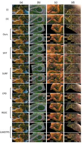
Figure 11.Registration examples on four typical image pairs from dataset (ii). The first two rows: the sensed and reference image. Within each two rows from third to twelfth, upper: the transformed image; lower: the checkboard.
3.4. Reliability and Availability Examination of Our Method
Figure 12.Registration examples on the seven typical satellite image pairs. From (a) to (g) are: Berlin, Las Vegas, Mekong River, Paris, WuHan, Washington and Hawaii. Columns from left to right are: the sensed, reference and transformed images, the checkboards, and the feature matching results. Blue lines indicate true positive and true negative, red lines indicate false positive and false negative.
Table 5. Experimental results on series (III). Quantitative tests on feature matching and image registration are carried out to examine the availability and robustness of our method using the PR, RMSE, MAE and SD. (a) to (g): results on the corresponding pairs of Figure12. Mean: the mean of results on all image pairs of dataset (iii). All units are in percentage.
(a) (b) (c) (d) (e) (f) (g) Mean
PR 96.88 96.77 95.97 95.77 95.09 98.19 95.57 96.54
RMSE 0.8358 1.3963 1.9556 1.4272 0.7743 1.4342 0.3171 1.1628
MAE 2.1458 4.0208 2.9097 1.9317 2.5778 2.3542 2.2958 2.6051
SD 1.8562 2.5498 2.5171 1.8061 2.1429 2.0098 2.0717 2.1362
4. Conclusions
In this paper, we proposed an accurate method for remote sensing image registration with different viewpoint. The main contributions of this paper are considered as follows. (i) The MGMM is constructed for simultaneously dealing with different types of image features. (ii) Two types of features are using to form a feature complementation, i.e., the Euclidean distance and shape context to measure the global and local geometric structure discrepancies, and the SIFT distance which is endowed with the intensity information are combined and substituted into the MGMM by which the reliable correspondence is obtained. (iii) To prevent the ill-posed problem, a geometric constraint term based on coherent velocity field is introduced into the L2E-based energy function and achieves accurate transformation updating. Experiments on three series of remote sensing images obtained from the unmanned aerial vehicle (UAV) and Google Earth with different viewpoint demonstrate that our method shows best registration performances against five state-of-the-art methods.
Yunnan Normal University [01000205020503065]; (iv) National Undergraduate Trainking Program for Innovation and Entrepreneurship [201610681002].
Author Contributions: Yang Yang, Anning Pan and Su Zhang developed the method; Kun Yang, Anning Pan and Su Zhang conceived and designed the experiments; Kun Yang, Su Zhang and Anning Pan performed the experiments and analyzed the data; Sim Heng Ong and Haolin Tang helped technology implementation of the method; Su Zhang and Yang Yang wrote the paper. All the authors reviewed and provided valuable comments for the manuscript.
Conflicts of Interest:The authors declare no conflict of interest.
References
1. Zitova, B.; Flusser, J. Image registration methods: a survey. Imag. Vis. Comput.2003,21, 977–1000. 2. Brown, L. A survey of image registration techniques. ACM Comput. Surv.1992,41, 325–376. 3. Maintz, J.; Viergever, M. A survey of medical image registration. Med. Imag. Anal.1998,2, 1–36.
4. Wang, X.; Li, Y.; Wei, H.; Liu, F. An asift-based local registration method for satellite imagery. Remote Sens.
2015,7, 7044–7061.
5. Liu, S.; Tong, X.; Chen, J.; et al. A Linear Feature-Based Approach for the Registration of Unmanned Aerial Vehicle Remotely-Sensed Images and Airborne LiDAR Data.Remote Sens.2016,8, 82.
6. Sedaghat, A.; Mokhtarzade, M.; Ebadi, H. Uniform Robust Scale-Invariant Feature Matching for Optical Remote Sensing Images.IEEE Trans. Geosci. Remote Sens.2011,49, 4516–4527.
7. Jensen, J.Introductory digital image processing; Prentice Hall: Upper Saddle River, NJ, USA, 2004.
8. Mikolajczyk, K.; chmid, C. A performance evaluation of local descriptors. in Proc. IEEE Conf. Comput. Vis. Pattern Recognit.2003,2.
9. Fan, B.; Wu, F.; Hu, Z. Rotationally Invariant Descriptors Using Intensity Order Pooling. IEEE Trans. Pattern Anal. Mach. Intell.2011,34, 2031–2045.
10. Harris, C. A combined corner and edge detector. in Proc. Alvey. Vis. Conf.1988,1988, 147–151.
11. Lowe, D. Object recognition from local scale-invariant features. in Proc. IEEE Int. Conf. Comput. Vis.1999,
2.
12. Lowe, D. Distinctive Image Features from Scale-Invariant Keypoints.Int. J. Comput. Vis.2004,60, 91–110. 13. Goncalves, H.; Corte-Real, L.; Goncalves, J. Automatic Image Registration Through Image Segmentation
and SIFT.IEEE Trans. Geosci. Remote Sens.2011,49, 2589–2600.
14. Bay, H.; Ess, A.; Tuytelaars, T.; Van Gool, L. Speeded-Up Robust Features (SURF). Comput. Vis. Imag.
Underst.2008,110, 346–359.
15. Li, Q.; Wang, G.; Liu, J.; Chen, S. Robust Scale-Invariant Feature Matching for Remote Sensing Image Registration.IEEE Geosci. Remote Sens. Lett.2009,6, 287–291.
16. Sedaghat, A.; Mokhtarzade, M.; Ebadi, H. Uniform Robust Scale-Invariant Feature Matching for Optical Remote Sensing Images.IEEE Trans. Geosci. Remote Sens.2011,49, 4516–4527.
17. Ke, Y.; Sukthankar, R. PCA-SIFT: A more distinctive representation for local image descriptors. in Proc.
IEEE Conf. Comput. Vis. Pattern Recognit.2004,2, 506–513.
18. Dellinger, F.; Delon, J.; Gousseau, Y.; Michel, J. SAR-SIFT: A SIFT-Like Algorithm for SAR Images. IEEE
Trans. Geosci. Remote Sens.2015,53, 453–466.
19. Liu, F.; Bi, F.; Chen, L.; Shi, H. Feature-Area Optimization: A Novel SAR Image Registration Method. IEEE Geosci. Remote Sens. Lett.2016,13, 242–246.
20. Gong, M.; Zhao, S.; Jiao, L.; Tian, D. A Novel Coarse-to-Fine Scheme for Automatic Image Registration Based on SIFT and Mutual Information. IEEE Trans. Geosci. Remote Sens.2014,52, 4328–4338.
21. Liu, Z.; An, J.; Jing, Y. A simple and robust feature point matching algorithm based on restricted spatial or derconstraints for aerial image registration.IEEE Trans. Geosci. Remote Sens.2012,50, 514–527.
22. Ma, J.; Zhao, J.; Tian, J.; Bai, X.; Tu, Z. Regularized vector field learning with sparse approximation for mismatch removal. Pattern Recognit.2013,46, 3519–3532.
23. Ma, J.; Zhao, J.; Tian, J.; Yuille, A.; Tu, Z. Robust point matching via vector field consensus. IEEE Trans.
24. Fischler, M.; Bolles, R. Random Sample Consensus: A Paradigm for Model Fitting with Applications to Image Analysis and Automated Cartography. Comm. of the ACM1980,24, 381–395.
25. Myronenko, A.; Song, X. Point set registration: coherent point drift. IEEE Trans. Pattern Anal. Mach. Intell.
2009,32, 2262–2275.
26. Liu, H.; Yan, S. Common visual pattern discovery via spatially coherent correspondences.in Proc. IEEE
conf. on Comput. Vis. and Pattern Recognit.2010, pp. 1609–1616.
27. Zhang, Z.; Yang, M.; Zhou, M.; Zeng, X. Simultaneous remote sensing image classification and annotation based on the spatial coherent topic model. IEEE Int. Geosci. Remote Sens. Symp.2014, pp. 1698–1701. 28. Ma, J.; Qiu, W.; Zhao, J.; Ma, Y. Robust, Estimation of Transformation for Non-Rigid Registration.IEEE
Trans. Signal Proc.2015,63, 1115–1129.
29. Ma, J.; Zhou, H.; Zhao, J.; Gao, Y.; Jiang, J.; Tian, J. Robust Feature Matching for Remote Sensing Image Registration via Locally Linear Transforming. IEEE Trans. Geosci. Remote Sens.2015,53, 6469–6481. 30. Yang, Y.; Ong, S.; Foong, K. A robust global and local mixture distance based non-rigid point set registration.
Pattern Recognit.2015,48, 156–173.
31. Lowe, D. Distinctive image features from scale-invariant keypoints. Int. J. Comput. Vis.2004,60, 91–110. 32. Sedaghat, A.; Ebadi, H. Remote Sensing Image Matching Based on Adaptive Binning SIFT Descriptor.
IEEE Trans. Geosci. Remote Sens.2015,53, 5283–5293.
33. Goncalves, H.; Corte-Real, L.; Goncalves, J. Automatic Image Registration Through Image Segmentation and SIFT.IEEE Trans. Geosci. Remote Sens.2011,49, 2589–2600.
34. Belongie, S.; Malik, J.; Puzicha, J. Shape Matching and Object Recognition Using Shape Contexts.IEEE Trans. Pattern Anal. Mach. Intell.2002,24, 509–522.
35. Kortgen, M.; Park, G.; Novotni, M.; Klein, R. 3D shape matching with shape context. in Proc. Cent. Eur.
Sem. Comput. Graph.2003, pp. 22–24.
36. Tikhonov, A.; Arsenin, V.Solutions of Ill-Posed Problems; Winston and Sons: Washington, D.C, USA, 1977. 37. Scott, D. Parametric statistical modeling by minimum integrated sqaure error. Technometrics2001,
43, 274–285.
38. Yuille, A.; Grzywacz, N. A Mathematical Analysis of the Motion Coherence Theory. Int. J. Comput. Vis.
1989,3, 155–175.