Swirling and non-swirling flow in conical diffusers

City, University of London Institutional Repository

Citation

:

This is the submitted version of the paper.

This version of the publication may differ from the final published

version.

Permanent repository link:

Link to published version

:

Copyright and reuse:

City Research Online aims to make research

outputs of City, University of London available to a wider audience.

Copyright and Moral Rights remain with the author(s) and/or copyright

holders. URLs from City Research Online may be freely distributed and

linked to.

SWIRLING AND NON-SWIRLING FLOW

IN CONICAL DIFFUSERS

N.E.A. WIRASINGHE

A th e s is presented f o r the degree o f

Doctor o f Philosophy o f The C ity U n iv e rsity .

Department o f Mechanical Engineering,

The C ity U n iv e rsity ,

2

ABSTRACT

The performance of conical diffusers with axial and

swirling flew has been considered. As a necessary starting point

the various criteria used for defining performance have been

reviewed and have been extended to swirling flew cases. A new

'AREA-PLOT' method, which unifies presentation of performance

information, for plane and conical diffusers has been preposed.

An added attraction of this method is that it displays all three

geometric variables of the diffusers.

As swirl modifies the boundary layer it was necessary to

have seme knowledge of the growth of the boundary layer in the axial

flew situation. This was achieved by extending the 'ROSS-FRASER'

model as a closed form solution requiring only the initial boundary

conditions. The predictions compare very well with published

experimental results.

The swirling flow case has been considered both

mathematically and experimentally, the latter being studied through

flew visualisation and measurement. An extensive survey of available

literature, on theoretical and experimental work, has been presented

with particular emphasis on areas not covered by previous surveys.

The mathematical analysis was aimed at identifying the dominant

parameters. The solution indicates the preferred coordinate system

and the possibility of further extension. It has been shown that

it is possible to represent the tangential velocity distribution

Further analysis indicated that the divergence of the solid-body

rotation core was parallel to the wall of the diffuser.

Flew visualisation studies have identified breakdown

and non-breakdewn areas in turbulent swirling pipe flow. The

development of the various modes of breakdown have been recorded.

Detailed flew measurement in the 10° diffuser indicates that

swirl has a definite effect on eliminating separation tendencies.

It was found that swirl modifies the wall static pressure drop in

PRINCIPAL NOMENCLATURE.

a Radius of crank of slider-crank mechanism

A Constant; cross-sectional area of duct

AR Area ratio (= A^/A^)

B,C,k Constants

y

R

2

Skin friction coefficient

Pressure recovery coefficient

Ideal pressure recovery coefficient

Coefficient of performance

Shape parameter

General function

Exponent (function of |R0O ); General function

Shape parameter ( =

0/0

Calibration factor associated with spherical probe

Mixing length; length of link of slider-crank mechanism

Slant length of diffuser

Angular momentum

= l/a as applied to slider crank mechanism

Static pressure

Mean static pressure

Mean axial kinetic energy

Mass flux through a region in the boundary layer

Mass flux through a cross-section

Radial co-ordinate

Radius of duct

Reynolds number

5

SR Non-dimensional wetted surface area

t time

u Axial velocity

u Mean axial velocity

u Peak value of axial velocity profile

u Friction velocity (=

J%jp

V Total velocity

W Radial velocity

y Distance measured radially from wall

Y Thickness of boundary layer

z Axial co-ordinate

Greek Symbols

fl Non-dimensional axial length (= z/Rq ); Angle of yaw

Radius ratio (= r/R or (r/krcf as indicated); Angle of pitch

y

0

j

vector and a given point on sphere

y * Axial kinetic energy factor

y** Axial momentum factor

<3 Dihedral angle; Boundary layer displacement thickness

€ Overall effectiveness; Eddy viscosity

C

7) Nondimens ional boundary layer co-ordinate

T)

7)e Energy efficiency

0

6

Diffuser loss coefficient

r Circulation

p

c0

V

P Density T Shear stress

4>

*

$ Projected maximum swirl angle [ T a n (Rco/u ) ]

CO Angular velocity

Q Circulation number (= R f / ü )

Superscripts

* Swirl case

1

[ ] Partial differential

Subscripts

c Conical diffuser; Value at inviscid core or at

"solid-body rotation" core

CL Centreline

d Based on diameter

i General case

p Plane diffuser

w Value at wall

Q

laminar sub-layer profile to y =

6

oo Inviscid flew outside boundary layer

ACKNOWIEDGEMENTS

The author wishes to extend his grateful thanks

to Dr. R.S. Neve for his guidance and encouragement

throughout this project.

The assistance of Mr. J.A. Snell, with computing,

and of Dr. A.W. Gillies, with mathematical work, is

acknowledged. The author is extremely grateful to Mr. R.

Chapman for developing the control system and to Mr. H.E.

Hart and his staff for their assistance with building the

test apparatus. Thanks are also extended to all those who

have assisted at various times including the library staff

and the computer staff.

Finally thanks are due to Mrs. K. Ahtuam for the

efficient manner in which this manuscript was typed and to

the Senate of The City University for granting the

CONTENTS Page.

ABSTRACT 2

PRINCIPAL NOMENCLATURE

4

ACKNOWLEDGEMENTS

7

CONTENTS

8

LIST CF FIGURES 13

LIST OF TABLES

CHAPTER I ; INTRODUCTION 19

CHAPTER 2 ; ESTIMATION AND PRESENTATION OF DIFFUSER

PERFORMANCE INFORMATION 27

2.1 Introduction 27

2.2 Axial flew at entry 27

2.3 A unified method for correlating performance

data for plane and conical diffusers 30

2.3.1 Introduction 30

2.3.2 Methods already in use 30

2.3.3 The 'AREA-PICT' method 35

2.4 Swirling flow at entry 37

2.5 Conclusions 41

CHAPTER 3 : BOUNDARY LAYER GROWTH IN A CONICAL DIFFUSER

WITH AXIAL FLOW 45

3.1 Introduction 45

3.2 Method of the Pennsylvania State University

Group 46

3.3 Ross's two dimensional model 47

3.3.1 Introduction 47

9

3.3.3 Growth of Flew Parameters 49

3.4 Fraser's three dimensional model 51

3.4.1 Introduction 51

3.4.2 Modification to Boss's equations 52

3.4.3 Method of solution 53

3.4.4 Limitations and conclusions 53

3.5 Extensions to the 'Fraser-model' 55

3.5.1 Basis of extension 55

3.5.2 Velocity profiles 56

3.5.3 Mass flux and core-velocity 58

3.5.4 The axisyirmetric momentum thickness 60

3.5.5 Computation of boundary layer parameters 60

3.5.6 Discussion and comparison 63

CHAPTER 4 : SWIRLING FLOWS; IÎ.TIODUCTION AND LITERATURE

SURVEY 73

4.1 Introduction 73

4.2 The vortex breakdown phenomenon 75

4.3 Survey of experimental work 78

4.3.1 Swirling flow in pipes 78

4.3.2 Swirling flew in conical diffusers 83

4.3.3 Swirling flew in Annular diffusers 91

4.3.4 Swirling free-jets 92

4.4 Conclusions 93

CHAPTER 5 ; THEORETICAL ANALYSIS OF SWIRLING FLOW 95

5.1 Introduction 95

5.2 Survey of prediction methods 96

5.3 Solution of the equations of motion for laminar

swirling flew in a conical diffuser.

Page

10

5.3.1 Governing equations 105

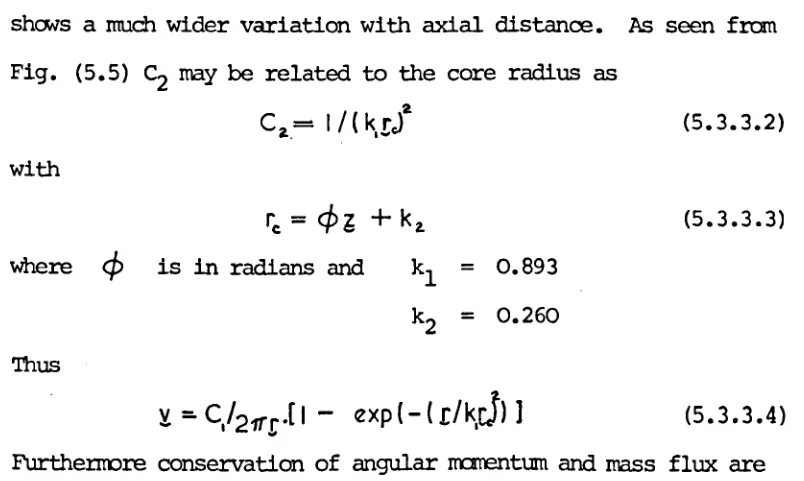
5.3.2 The swirl distribution 106

5.3.3 Decay of swirl intensity 107

5.3.4 Method of solution 114

5.3.5 The static pressure distribution 116

5.3.6 Discussion of solution

117

5.4 Conclusions

119

CHAPTER

6

6.1 Design considerations 124

6.1.1 Basic requirements 124

6.1.2 Scale and flexibility of test rig 124

6.2 Test-Rig 126

6.2.1 General arrangement 126

6.2.2 Swirl generation 133

6.2.3 'Universal' coupling for probe-carrier 139

6.2.4 Probe traversing mechanism 140

6.3 Instrumentation and calibration 153

6.3.1 Measurement of mean flew-rates and

turbulence 153

6.3.2 Speed control of swirl generator drive

motor 157

PRECAUTIONARY MEASURES = ---

1

FLOWS 168

7.1 Introduction 168

11

Paçje

7.3 Probes in yaw and pitch measurement 170

7.3.1 Flew past a sphere 170

7.3.2 Presentation of calibration curves 172

7.3.3 Coordinate system 176

7.4 Calibration equipment 177

7.4.1 Design considerations 177

7.4.2 Probes used and calibration tunnel 178

7.5 Calibration and analysis 182

7.6 Conclusions 190

CHAPTER

8

8.1 Introduction 191

8.2 Flow visualisation and tracer agents 192

8.3 Experimental apparatus 195

8.4 Experimental work 196

8.5 Observations 199

8.5.1 The development of vortex breakdown 199

8.5.2 Vortex breakdown in a diffuser 208

8.5.3 The travelling primary core-head

211

8.6

CHAPTER 9 : MEASUREMENT OF FLOW IN DIFFUSERS 217

9.1 Introduction _ 217

9.2 Experimental apparatus 217

9.3 Evaluation of flew properties 218

9.4 Performance of swirl generator 220

9.5 Flow in the 10° diffuser 225

12

Page

9.7.1 Basic assumptions 237

9.7.2 Diffuser performance 240

9.8 Discussion and conclusions 240

CHAPTER 1 0 : CONCLUDING COMMENTS 249

10.1 Aims and method of investigation 249

10.2 Results 249

10.3 Guidelines for future research 252

REFERENCES 256

TABLES 262

13

LIST OF FIGURES

CHAPTER I

page

1.1 Diffuser efficiency; Peters (1934) 22

1.2 Flew chart displaying scope for research

associated with diffusers 24

CHAPTER 2

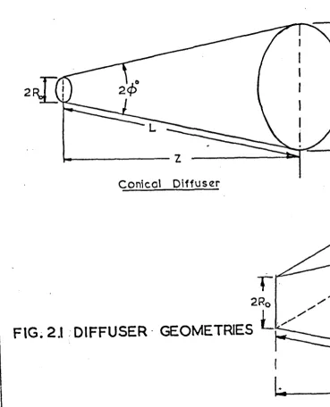
2.1 Diffuser geometries 31

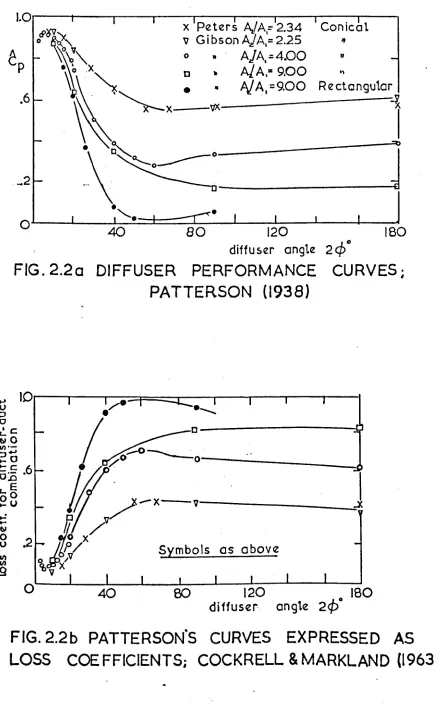
2.2.a. Diffuser performance curves; Patterson (1938) 32

b. Patterson's curves expressed as loss coefficients;

Cockrell and Markland (1963)’ 32

2.3 Significance of squared terms in equation (2.3.2.

6

2.5 Typical performance curves for plane diffusers; Fox

and Kline (1962) 38

2.6 Conical diffuser performance without swirl; McDonald

and Fox (1966) 39

2.7 Performance of conical diffusers - 'AREA-PLOT' 42

2.8 Flew regimes in conical diffusers; Axial flew;

McDonald and Fox (1966) 43

2.9 'AREA-PLOT' presentation of flow regimes in diffusers 44

CHAPTER 3

3.1 Division of velocity profile in boundary layer 50

3.2 Variation of (2 + G) with IRgo 50

3.3 Curve for determining D. 64

3.4 Coordinates used in duct. 64

Page 3.6 Velocity distribution in boundary layer

68

68

3.9 Simplified flow chart - Master 'BLID' 72

CHAPTER 4

4.1 The two forms of vortex breakdown 77

4.2 The spiral and axisynmetric modes of breakdown;

L a m b o u m e and Bryer (1961) 79

4.3 Swirl instability in laminar pipe flew; Talbot (1954) 80

4.4.a Diffuser "under" efficiency; Liepe (1966)

b Diffuser flew regimes; Liepe (1960) 85

4.5 Effect of swirl on (a) Diffuser performance 90

*

(b) Contours of constant C p = 0.70 90

(c) Line of optimum performance G - G 90

CHAPTER 5

5.1 Computer fit of exponential function to diffuser data 109

5.2 Computer fit of exponential function to pipe data 110

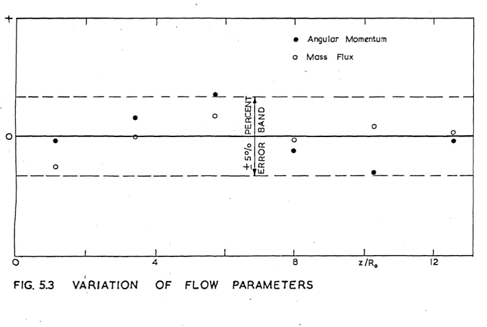
5.3 Variation of flew parameters 111

5.4 Divergence of core-radius 112

5.5 Variation of constants of tangential velocity

function 113

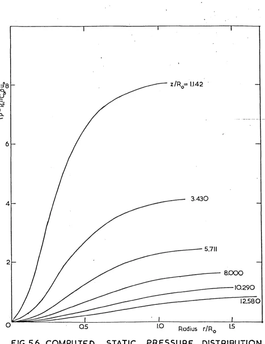
5.6 Computed static pressure distribution in diffusers 118

5.7 Variation of turbulent viscosity in pipe flew;

SCHLINGER (1953) 121

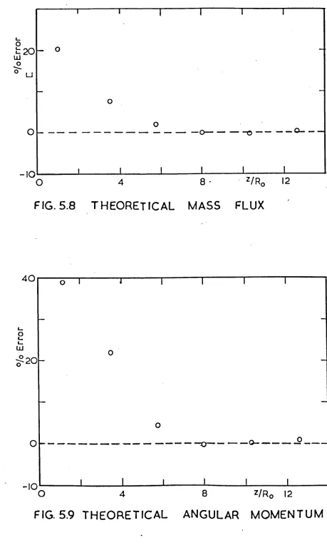
5.8 Theoretical mass flux 122

14-15

6.1 Overall dimensions of test-rig 127

6.2 Layout of test rig 128

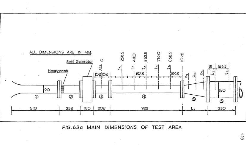
6.2a Main dimensions of test area 129

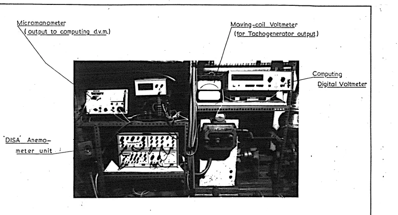
6.3 Recording instruments used for experimentation 130

6.4 Gwynnes centrifugal pump characteristics 132

6.5 Exploded view of swirl generator 135

6.6

6.7 Swirl generator assembly 138

6.8

6.9 Angular divisions used for stepping motion 144

6.10 Sensitivity of harmonic motion 145

6.11 and 6.11a Probe traversing mechanism 147

6.12 and 6.12a Diffusers used in experiments 149

6.13 Electro-mechanical control system for traverse

mechanism 152

6.14 Orifice plate calibration curve - air 154

6.15 Orifice plate calibration curve - water 155

6.16 Orifice plate calibration curve - water 156

6.17 Control system for speed variation 159

6.18 Effect of thyristor on A.C. output 159

6.19 Method of obtaining pulses 161

6.20 Circuit used in speed control system 162

6.21 Layout of electronic circuit 163

6.22 Method of speed control via feed-back 164

6.23 Calibration curve; Swirl generator drive motor

CHAPTER 6 Page

16

7.1 The five-hole spherical probe 171

7.2 Drill jig for hemispherical probe head 179

7.2a The hemispherical pitot probe 179

7.3 The calibration tunnel 181

7.4(a, b, c)Characteristics of hemispherical pitot probe 183

7.5 Calibration curve for hemispherical probe 187

7.6 Curves shewing suitability of P

2

balancing probe 188

7.7 Swirl angle and static pressure measurements using

hemispherical probe 189

CHAPTER

8

8.1 Size distribution of polystyrene 'waste' 197

8.2 Arrangement for photography 200

8.3 Development of vortex breakdown in pipe flew 203

8.4 Development of vortex breakdown in pipe flow 209

8.5 Flew regimes in swirling pipe flow 210

8.6

8.7 Vortex breakdown in a diffuser - Sarpkaya (1971) 215

CHAPTER 9

9.1 Variation of tangential velocity with speed of

swirl generator (as measured at st.l in

10

221

9.3 Variation of flow properties for above case 224

9.4 Axial velocity distribution in 10° diffuser 226

9.5 Tangential velocity distribution in 10° diffuser 227

9.6 Variation of flow properties in 10° diffuser;

swirl 228

17

9.7 Variation of flow properties in 10° diffuser;

axial flew

9.8 Wall-static pressure drop in inlet pipe

9.9 Wall-static pressure in diffuser and tail-piece

9.10 Pressure variation in diffuser-pipe combination

9.11 Diffuser performance with swirl

Pase

229

231

232

241

LIST OF TABLES

CHAPTER 3 Page

3/1 Diffuser boundary layer data; Fraser (1958) 262

3/II Diffuser boundary layer data; Computed 263

3/III Computed velocity profiles 264

CHAPTER 5

5/1 Carputed flow properties for

6

7/1 Probe characteristic data - Refer Fig. 7.4 266

CHAPTER 9

9/1 Flew properties with increasing swirl 267

9/II Data for 10° diffuser - Axial flow 268

9/III Data for 10° diffuser - Swirl 2 269

CHAPTER I

INTRODUCTION

In fluid mechanics, a duct in which the cross-sectional

area increases in the direction of flow is termed a diffuser. In

subsonic flews it decelerates the flow with an accompanying

increase in static pressure. Which of these is the primary

objective is dependent on the particular application; however each

of these objectives needs to be achieved with the minimum of

losses. Almost any basic contour may be used to achieve this

expansion; the conical diffuser however has been used extensively

owing to its simple geometry which makes it attractive in practical

applications.

Despite the vast amount of research over the years, the

basic characteristics of flew in a diffuser are still not clearly

understood. Whilst it is desirable to employ an optimum diffuser

where possible (i.e. one which yields the highest pressure

recovery coefficient), in practice other design considerations

preclude this and sometimes it is necessary to employ an other

than optimum diffuser. This more immediate requirement of the

design engineer has been satisfied by providing performance charts

in which the pressure recovery coefficient, defined as

c p= (P.-P.i/q,

is given as a function of the area ratio and expansion angle (or

20

In major industrial applications even a few percent

improvement of efficiency represents a significant financial

saving and therefore factors influencing diffuser performance are

eagerly sought. Early researchers were of the view that performance

was a function only of the gecmetry of the diffuser. However,

recent work has shewn that the thickness of the inlet boundary

layer and the level of inlet turbulence are also relèvent parameters.

The adverse pressure gradient associated with flow in the diffuser

thickens the boundary layer and can lead to separation. In

separated flews the kinetic energy available for conversion to

flew work is lost as internal energy.

Over the years various methods have been employed to

prevent boundary layer separation. Of these, boundary layer

suction in particular has received a great deal of attention.

This removal of Slew moving fluid from the boundary layer causes

high velocity fluid fran the core region to replace it. The

greater kinetic energy of this fluid enables it to overcome the

effects of the pressure gradient thus preventing separation.

Ackeret (1958), Furruya, et. al. (1966) and several others have

improved performance by this method. Moon (1958) reported that

suction was effective only with thin entry boundary layer

thickness and that suction was totally ineffective when this was

excessively thick.

Several other isolated methods have been used iron time

to time. Persh and Bailey (1954) increased wall roughness while

both claim iirprovements. Improvements have also been claimed for

wide angle diffusers by Yang (1965) who suspended an axisyirmetric

aerofoil centrally inside the diffuser. The effect of screens on

performance was investigated by W i n t e m i t z and Ramsey (1957) and

Moore and Kline (1958). Sprenger (1959), Senoo and Nishi (1974)

and several others used vortex generators to improve diffuser

performance. These were used only in specific applications and a

vast amount of experimentation isrequired to determine the

optimum configuration of vortex generators and to quantify the

benefits.

According to Peters (1931

),

redistributing energy though the latter did not venture to

investigate this any further. Peters himself carried out some

preliminary work to investigate this view. As seen from Fig. (1.1),

swirl in fact does improve performance. Later, work by Liepe (1960)

and Van Dewoes tine (1969) further reinforced this view.

The current research programme arose from the view that

it may be possible to improve the performance of the fluidic vortex

amplifier by attaching a diffuser to its exit. The discharge from

a switched vortex amplifier possesses a high degree of swirl and

the aim is to generate a higher impedence in the chamber by diffusing

the discharge. Following recent work on the performance of fluidic

vortex amplifiers by Neve (1971) it was decided to conduct

a comprehensive research programme to investigate the character of

swirling flew in diffusers and in a pipe (diffuser with zero

divergence angle

),

E

ff

ic

ie

n

c

y

FIG.U DIFFUSER

EFFICIENCY ; PETERS ( 1934 )

23

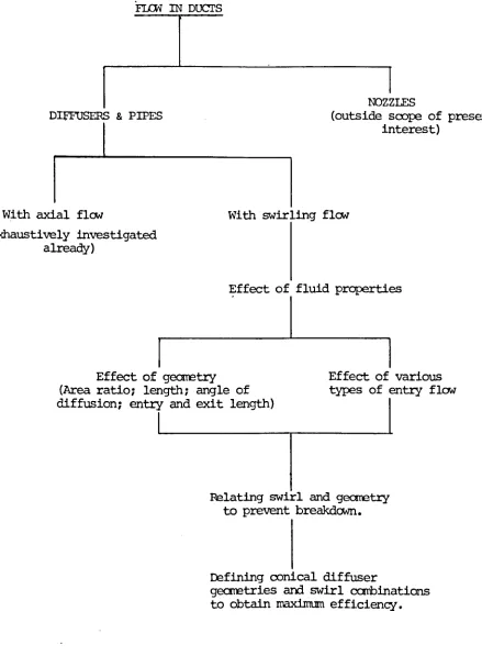
Flew in ducts covers a major portion of the subject of

fluid mechanics. As Fig. (1.2) indicates, even when restricted

to conical diffusers the subject is extremely wide. It is

obviously inpossible to build one universal test apparatus to

investigate the entire problem. Each individual project, within

the main programme, should investigate a few of the parameters at

a time thus providing the necessary information to put this subject

on a similar footing to that of diffuser performance with axial

flew. Cwing to the almost non-existent expertise in this field,

laying a suitable foundation was seen as an absolute necessity.

Ihe present project was seen as one that would make a global

assessment of the programme in addition to performing a steering

function for future research in this field.

A considerable degree of ambiguity still exists in the

manner in which diffuser performance is evaluated. In Chapter Two

the various criteria have been developed logically in an attempt

to coordinate these. Parallel criteria have also been developed

for evaluating performance of diffusers with swirling flow. A

new 'AREA-PLOT' method unifying presentation of such information,

in two and three dimensional flews, has also been developed.

The boundary layer growth in the conical diffuser, with axial flew,

is considered analytically, in Chapter Three, by extending the work

of previous investigators to obtain a closed form solution. The

special numerical techniques developed are also included but the

24

FLOW IN DUCTS

DIFFUSERS & PIPES

NOZZLES

(outside scope of present interest)

With axial flow

(exhaustively investigated already)

With swirling flew

Effect of fluid properties

Effect of geometry (Area ratio; length; angle of diffusion; entry and exit length)

Effect of various types of entry flow

Relating swirl and geometry to prevent breakdown.

Defining conical diffuser

geometries and swirl combinations to obtain maximum efficiency.

Fig. 1.2 FLOW CHART DISPLAYING SCOPE FOR RESEARCH ASSOCIATED

25

The characteristics of swirling flow and the associated

vortex breakdown phenomenon are introduced in Chapter Four. An

extensive survey of relevant previous experimental work is

presented. Included is a discussion on the role of swirling flow

in jets, pipes, conical diffusers and annular diffusers. Ctoing

to the scarcity of experimental data mathematical analysis of the

swirling flew problem has been stunted. Most of the prediction

methods proposed have attempted to predict the occurrence of vortex

breakdown. Only a few have attempted to study decay of swirl.

These methods have been reviewed in Chapter Five. Furthermore the

governing equations of motion have been solved to investigate the

influence of dominant parameters in laminar swirling flow in

conical diffusers.

During the design stages of the test apparatus and

instrumentation, it was decided not to limit the scope of the

apparatus to this project alone but to endeavour to make it

sufficiently flexible to accommodate as much of the forseeable

future programme as possible. Consequently convenience had to be

sacrificed for greater latitude of experimentation. Design

information is reported in detail in Chapter Six. As the five-hole

pitot probe used for measurement was the subject of a more detailed

analysis, it is discussed separately in Chapter Seven.

Chapter Eight describes the flew visualisation work

conducted in water to observe the development of vortex breakdown.

Ihe discussion throws light on the difficulties associated with

such work. Experimental work associated with flew measurement in

Diffuser performance information is also included with comparisons,

where possible.

The work carried out is reviewed in Chapter T e n / and the

results are presented. Possible extensions in the various areas

CHAPTER TWO

ESTIMATION AND PRESENTATION OF DIFFUSER

PERFORMANCE INFORMATION

2.1

As diffusers are concerned with obtaining as much static

pressure as possible iron the kinetic energy of the fluid their

functional efficiency must be measured accordingly. Various

definitions for such measurements have been proposed in an attempt

to obtain a convenient method for presenting performance information.

As a result a certain degree of ambiguity has been introduced. In

an attempt to resolve this the various definitions used for

measurement of performance are derived in a logical manner. The

validity of same of the terms used will always remain arguable

though this is of secondary Importance. The subsequent discussion

will also concentrate on developing a suitable basis for presenting

such information when the flew at entry to the diffuser possesses

a swirl component of velocity. In addition an improved 'AREA-PLOT'

method has been developed for presenting performance information.

2.2_______AXIAL FLOW AT ENTRY

efficiency' of a diffuser be defined as the ratio of the power

transformed to the power supplied for transformation.

Patterson (1938) suggested that the 'overall energy

28

If the flew is axial at inlet and outlet sections

then V = u and, as the uniform pressure is in addition

transmitted through the boundary-layer, the above equation yields

the 'energy efficiency'.

Using the kinetic energy (weighting) factor

y

f udA

*

K

this becomes

\ =

where AR =

AjA^

ptf/2

is uniform at the initial and final sections then % * % ! = ■ I

and equation (2.2.3) reduces to the 'coefficient of performance'

C p = (pa- R ) / q t(!-ARJ" (2.2.4)

In real flews in ducts the presence of the boundary layer

causes a non-uniformity of velocity. As a consequence of its

definition y ^ will always be greater than unity and in the case

of the paraboloid velocity distribution associated with fully

developed laminar flows % = 2. In the case of a thin inlet

boundary layer may be assumed to be unity but such an assumption

is invalidated at the exit of a diffuser where the adverse pressure

gradient creates a very thick boundary-layer.

i/

TH-In a typical case using the

77

u/u =■ (I — r/R )

yields

=

approximation to test data given by

* m

29

which for m = 2 yields % = 1.045. Even though y ^ is

always greater than y ^

,

-1 -2

A R is less than unity and A R is very much less than unity.

Applying this condition and the assumption that y ^ =

1

c p=

<2-2-5>

which has been used frequently as it obviates the need to

evaluate velocity profile data at exit.

For flew in a diffuser, under uniform conditions, the

Bernoulli equation with a loss term A p is

p, + q* =

and in the ideal case this becomes

p, + q, = Pa+q*

Invoking this ideal condition into equation (2.2.5) leads to the

'ideal pressure recovery coefficient'.

C p = I - A R 2 (2.2.6.)

Almost wholly, diffuser performance has been measured

in one or more of the above forms (or a modification of the above

forms). Sovran and Klcmp (1967) for example, suggested the use

of the diffuser "overall effectiveness" defined as

€

Clearly this is identical with the coefficient of

performance defined in equation (2.2.4). Cockrell and Markland

(1963) proposed the use of the "diffuser loss coefficient".

\

Thus it is seen that all the forms are approximations

30

2.3______ A UNIFIED METHOD FOR CORRELATING PERFORMANCE DATA OF

PLANE AND CCNICAL DIFFUSERS.

2.3.1 ___ Introduction

Systematic studies were carried out at Stanford

University with plane (two dimensional; Fig. (2.1)) diffusers

in an attempt to extend the knowledge gained to conical diffuser

flews. This attempt was greatly hindered by the lack of a suitable

basis for correlating performance information from these two types.

A

the three common geometric paramters; viz. area ratio, divergence

angle and length to inlet diameter ratio. In industrial situations

any one of these may be the constraining parameter. Quite often

the performance itself is the constraining parameter when

equipment dewnstream of the diffuser requires a prescribed input

pressure. If performance charts are not readily available in

the required form this would cause inconvenience.

2.3.2 Methods Already in Use

The method used by Patterson in his early review is

shewn in Fig. (2.2a). A similar method was used by Cockrell and

Markland, Fig. (2.2b). It is useful to note that in both cases

the length parameter has been considered to be the least important.

Recently at Stanford University contour plots were used, with plane

walled diffusers, in which all three parameters were readily

available. The simple geometric relationships of the plane

diffuser have made this possible.

---z

---Conieoi D iffu se r

T

2

0

*-32

FIG. 2.2a DIFFUSER PERFORMANCE CURVES;

PATTERSON (1938)

53

R = R0+ z Tan

(2.3.2.1)

For the plane walled diffuser the area ratio is

ARp = R / R

— J

(

.

.

.

)

and substituting this into equation (2.3.2.1) yields

ARp=| +(z/F^ Tan

(2.3.2.3)

or

I n (ARp-1 ) = ln(z/Rj +ln(Tanc£)

(2.3.2.4)

The use of logarithmic scales would result In the half

angles appearing as a series of parallel straight lines. Furthermore,

as the area ratio is always greater than unity, the region of greatest

practical interest, which is the region of smaller area ratios, is

stretched out by the use of (AR ~ I) as the ordinate. P

On the basis of the limited conical diffuser data

available at the time, Kline, Abbot and Fox (1959) postulated that

performance data for axisyirmetric flews could be correlated on the

same basis as the data frem two dimensional flews.

For a conical diffuser the area ratio is

2

A R C = ( R / F y = j8 (2.3.2.5)

and on substituting for R in equation (2.3.2.1) yields

AF\.= I + 2(z/k)Tan

4>

+ [(z/Fy Tan<£]*

6)

This expression would be similar to that given by

equation (2.3.2.3) provided the last term is negligible. Fig. (2.3)

which has been drawn with and without the last term of equation

(2.3.2.

6)

the contour plots provide an opportunity to present all three

parameters for plane diffusers they do not permit a similar

representation of conical diffuser information. This naturally

(

A

R

-I

J

35

2.3.3 The 'AREA-PLOT* Method

A new type of ‘AREA-PLOT' is suggested as a preferable

alternative to the previously discussed contour plots. The

ordinate is the flew area ratio and the abscissa is the ratio of

wetted surface area to inlet flew area. The introduction of a

new parameter, to add to the three already in existence, may at

first sight seem an added complication. However it will be shewn

that this permits the development of identical relationships for

both forms of diffuser.

Plane Walled Diffuser

Referring to Fig. (2.1) the slant length is

L = ( R “ F\j) / Sin

4>

and L / R Q= p - l ) / S i n < ^ >

The wetted area per unit width of diffuser is S = 2L

and the relevant wetted surface area ratio is defined as

SRp = 8/ 2Rq= 1/3 — I )/Sin<#>

frcm which

In (ARp- 1 ) = In (SRp) + ln(Sinc#>)

(2.3.3.1)

Conical Diffuser

Considering an element on the conical surface

z =■ L. C o s

4>

The wetted area is

Sc= 2 ir^ R .d L

= 2fl/(Rrt+z.Tanc£) dz/Cos<£ *b °

integrating and substituting for Z fran equation (2.3.2.1)

36

Also the flew area ratio is

A R c = ( R / R of = j0*

The relevant wetted surface area ratio is defined as

S R C = | / ir R o = ( £ * - I )/S\ncj>

from which

t n ( A R - l ) = In (SFy 4- In (Sinc^>) (2.3.3.2)

Equations (2.3.3.1) and (2.3.3.2) indicate that it is

new possible to correlate plane walled and conical diffuser results.

On these 'AREA-PLOTS', lines of constant nan-dimensional axial

length for the conical diffuser (not applicable to plane walled

diffuser) have been drawn as this is the case of greatest practical

interest. In addition to this correlation facility all the

parameters are new represented in these new plots. In view of the

small angles considered in practice it is suggested that Sinc£

be replaced by

cf>

I n ( A R - l ) - In (SR) + I n (<£) (2.3.3.3)

The error, in the geometric relationship of

(f)

(f> =cj>

for A R = 6, for a typical range of diffuser angles is as follows:

2

cf>°

It should be observed that for the plane walled diffuser

the expression obtained by the present method (equation (2.3.3.1))

and that used in the contour plots (equation (2.3.2.4)) are almost

equal as in the range of greatest practical interest T a n c £ « S l n < £

Hence for these, contour plots may be used as before with the

37

Figs.(2.4 and 2.5) shew the flew regimes for a plane walled

diffuser and a typical performance chart respectively. Figs.

(2.6. and 2.7) show a typical performance chart for conical diffusers

in the earlier and later type of plot.

axial flew at entry the "pressure coefficient" defined by equation

(2.2.5) may be used to estimate the error. It is arguable whether

the performance of a diffuser should be measured in terms of the

actual dynamic pressure used in the conversion process or in terms

of that which is required at input irrespective of the dynamic

pressure left at exit. The latter has been in carman use as it

obviates the need to evaluate velocity profile details at the exit

section.

For the swirling flew case the "overall energy efficiency"

is as defined by equation (2.2.1)

, ^2 2. Z

but V = u + v

and

p = pec+ pv^2

The angular momentum flux is

Considering the special case of solid-body rotation, v = rCO ,

this becomes

2.4 SWIRLING FLOW AT ENTRY

It was shewn that in the case of a conical diffuser with

(2.4.1)

Introducing the angular momentum (weighting) factor

M =)/

irp

oo G

7 2 =

2

irpoú£ur5dr

The flew work term in the numerator of equation (2.2.1)

F IG.2.4 FLOW REGIMES IN PLANE

DIFFUSERS

(

A

R

.

-I)

39

40

which, for the solid-body rotation case reduces to

f

pudA =■ CLP /p

+-C

M

•A (2.4.3)

The kinetic energy term in the denominator of

equation (2.2.1) is

P/2

.¡V

irpfo

P & j j V u d A » G L q ^ / p + 0 0 M / 2 (2.4.4) Substituting the above expressions into equation (2.2.1)

yields

* Q - ^ - g J / p + ( c q M e - o q M ) / 2 4 5)

°

- (WM

-W,M

If the angular momentum is conserved then

CL(p- p )/p 4-

- I )/2

7)= --- * » - ■--- LJ--- !--- (2.4.6)

Q.q(%( I ~ AR

M^Woo, - D

If only a very Jnild' swirl is inparted to the fluid

at entry then it may be assumed that the pressure distribution

is uniform across the section. Also if only the kinetic energy

at inlet is used as a reference, as is usually the case, then the

above equation reduces to the 'pressure recovery coefficient'

C p “ ( | - R ) / ( q , % , + P M “ ,/2Q ) (2.4.7)

This equation provides a very convenient basis for

ccmparison of performance, provided only 'mild' swirl is used,

as it does not require a detailed knowledge of the velocity

profile at exit. The validity of the assumptions made in reducing

41

2.5 CONCLUSIONS

It has been shewn that sane degree of ambiguity exists

in the estimation of diffuser performance; this being more serious

when swirl is present at inlet. An improved 1AREA-PLOT' has been

proposed for the presentation of performance information. Figs.

(2.4) and (2.5) shew the flew regimes and a typical performance

chart, respectively, associated with plane diffusers. Fig. (2.6)

shews a typical performance chart for a conical diffuser which

has been redrawn on the new plot on Fig. (2.7). The advantage of

the latter form is the appearance of the cone angles. Fig. (2.8)

shews the flew regimes associated with conical diffusers; this has

been redrawn on the new plot on Fig. (2.9). It is seen that if the

flow regimes in Figs. (2.4) and (2.8) are caipared the trends are

not easily apparent. If, hewever, Fig. (2.4) is corpared with Fig.

(2.9) the trends are obvious thus further justifying the use of

these plots. Comparison infaert, does indicate that the lines

of first appreciable stall for plane and conical diffusers do not

correspond to the same geometries. Further analysis is required

to determine whether or not it is possible to correlate performance

data for the two forms of diffuser. In concluding, it is worth

noting that all the previous investigators [ Peters (1931), Liepe

(1963) and Van Dewoestine (1969) ] emitted the exit velocity profile

details in evaluating performance (for swirling flow cases) owing

to the difficulty of measuring these. The use of angular momentum

flux instead of tangential velocity, in the evaluation of performance

with swirl, eliminates seme of the errors associated with

(

a

r

-i

.

(A

F

^

-I

)

S R C

8 0

Refer Fig.2.8 for symbols

tine of first

appreciable stall

5

IO

2 0

4 0

8 0

SRc

FIG.2.9 AREA-PLOT PRESENTATION OF FLOW REGIMES IN DIFFUSERS

k

s

CHAPTER THREE

BOUNDARY LAYER GROWTH IN A CONICAL DIFFUSER WITH AXIAL FLOW

3.1_______ INTRODUCTION

The lack of success in the attempts to predict the

flew in a conical diffuser could be attributed to the failure

to solve the governing equations of motion. The Navier-Stokes'

equations have been accepted universally as a basis for the

theoretical analysis of fluid dynamic problems. These were

first developed for laminar flow applications and later Osborne

Reynolds extended these to turbulent flow cases. He replaced

the laminar velocities and mean pressures by their instantaneous

counterparts. The resulting equations, generally known as

Reynolds * equations, had additional terms representing turbulent

transport of momentum known as Reynolds' stresses. The original

laminar equations, being non-linear, have been solved exactly

only for a very few cases. Now with the addition of the

turbulent stress terms such a solution is unimaginable.

Analytical approaches too have had only a limited degree

of success. Where a diffuser is concerned one factor largely

responsible has been the limited knowledge of the growth of the

turbulent boundary- layer in the presence of an adverse pressure

gradient.

This chapter deals with an analytical method for

46

of the model was developed Initially during an extensive

programme of research an flow in diffusers at the Pennsylvania

State University. This has been extended now to cbviate the

need for information an the core-velocity along the length of

the diffuser.

3.2_______METHOD OF TOE PENNSYLVANIA STATE UNIVERSITY GROUP

A programme of research was initiated in 1945 at the Pennsylvania State University in connection w ith the design of a high speed water-tunnel. Ross, w h o w a s associated w i t h this programme, postulated a new physical approach to the turbulent boundary-layer problems. This, combined w i t h empirical

correlations,, provided a method for evaluating two-dimensicnal- turbulent boundary-layer parameters in the presence of an adverse pressure gradient.

Fraser extended this quite successfully to three

dimensional flows. Within the range of validity of the method,

the predicted values of boundary layer parameters compared very

well with their experimental counterparts. Later Robertson and

Fraser proposed a method for diffuser design using Fraser's

model, based cn the occurrence of "separation" as the criterion

for determining the geometry of the diffuser. They went further

to suggest a method for predicting the performance coefficient.

The method involves using a set of graphs and equations

to evaluate the boundary-layer parameters, proceeding downstream

in a station-wise manner. It requires prior knowledge of the

that this could be calculated frcm experimentally obtained

static pressures at each station.

3.3______ FOSS'S TWO DIMENSIONAL MODEL

3.3.1 ___ Introduction

The method is based on a new approach to flow in the

boundary-layer. A three-zone division is considered based on

the relative influence of viscosity an flaw in the boundary layer.

He analysed a vast amount of experimental data frcm previous

investigations to obtain correlations between the growth of flew

parameters. As Ross (1956) has already discussed his method in

detail only the basis of his work will be discussed here since

it is the extensions made by Fraser (1958) into three

dimensional flews that are of major interest.

3.3.2 ___The Turbulent Boundary Layer Profile

Prandtl' s mixing length theory for momentum transfer

between various strata in a turbulent flow leads to the following

relationship for the dominant Reynolds stress:

T = -puV=pf!|du/dy|.du/dy (3.3.2.1)

Amongst others, an assumption of mixing length being

proportional to distance from the wall then leads to the well

known logarithmic velocity profile

u/iy= A lo g j uy/v) -I- B

(3.3.2.2)

where A and B have been determined experimental ly to be 2.5 and

5.6 respectively. Close to the wall the logarithmic term tends

to an infinitely negative value, but in this region a laminar

48

mixing length tending to zero because of the solidity of the

wall accords well with this fact. The three regions involved

in this analysis (the laminar sub-layer, logarithmic region and

a buffer zone) have known velocity profiles in a turbulent boundary

layer up to a height of about 7) = 0.1. From 7) = 0 . 2 5 to

7) = 1, equation (3.3.2.2) becomes progressively less

satisfactory, largely because the mixing length no longer retains

its proportionality to y but attains a constant value of about

0.14Y. Resort is usually then made to the 1/n-pcwer law, where n

depends an Reynolds nunber but is usually taken as 7, or to a 3

"wake" type profile, or to the - power law based on work by

Darcy

, 3/a

( l - u / u j = D .(I - y/Y ) (3 .3 .2 .3 )

where D is a shape factor which depends on the past history of

the flow.

It seems reasonable, therefore, to divide the boundary

layer not into regions which depend on the mixing length being

constant, proportional to y, or equal to zero but into regions

which are either dependent on past history of the boundary layer

and free-stream pressure gradient or influenced by the proximity

of the wall and independent of pressure gradient. In any

turbulent layer in an adverse pressure gradient, the profile from

the wall to about

7

is. Ross has therefore suggested that the breakdown shown in

Figure (3.1), which includes a blending region, dependent to

4-9

velocity profiles are made compatible. This latter condition

may often require an inflection, so the equation for this region

would need to be at least a cubic.

Ross states that for the outer turbulent region

(equation 3.3.2.3) an accurate idea of impending boundary layer

separation is given by the condition D = 1.3 + 0.1. This is

clearly equivalent to the shape factor H i « 6 I Q ) for the -y - pcwer lav profile tending to a separation value of about 3.5.

The substitution of a constant mixing length into

Prandtl's model leads to

D =[2/3][Y/l]7t/Pui (3.3.2.4)

and multiplication of both sides by U o/u<joo leads, after

rearrangement, to

, -i/a

[Y/D](uoayuJ=[3l/2]

[rjpul)

distance downstream fran the initial condition (suffix 0) and not

of local wall conditions; experimental results by Schubauer and

Klebanoff (1950) have confirmed this.

3.3.3_____Growth of Flow Parameters

The use of the vcn Karman integral momentum equation

d0/dz = ( 2 + H ).[0/pu*]{dp/dz]+Cf/2 (3.3.3.1)

in turbulent flows with adverse pressure gradients has already

resulted in poor approximations. It was originally derived for

use with laminar boundary- layers and has been applied quite

extensively to turbulent flows with seme degree of success.

However, it needs to b e modified before it can be applied

V D

FIG.3.1

DIVISION OF VELOCITY

E

X

P

O

N

E

N

T

(

2

t

-G

)

FIG.3.2 VARIATION OF(2+G] V/ITH Rs9o

vn

In view of the difficulty in solving such an equation

Ross preposed an empirical relationship for the growth of

momentum thickness,

2+G

9JQ

= (uc/u j

(3.3.3.

2

)

where G is a parameter dependent only an the inlet momentum

thickness Reynolds' nunber, Fig. (3.2) shows the variation of

(2 + G) with Pq which may b e represented by

(24G ) =0.0143(In \Rgf - 0 4 6 6 7 In IR,+7.554

(3.3.3.3)

Furthermore an the basis of the Prandtl momentum-

transfer theory and dimensional analysis, Ross showed the outer

velocity profile parameter D to be governed by,

tY/0D][uc/u J = [(A (v z )/0 J + vyeoD j [§/0]

(3.3.3.41

where A is a constant evaluated in the zero-pressure gradient

region ahead of the region of relatively strong pressure gradients.

Ross went on to show that

A -O .0 2 5 ( 1 + 12C fo)

(3.3.3.5)

If the initial velocity profile is knewn A may be

calculated by determining . By obtaining Y/0D, D could o

be read off Figure (3.3) which is an experimental curve provided

by Ross from several sets of data. Now the problem is one of

solving a series of algebraic equations with the aid of seme

experimental curves.

As pointed out by Ross himself, the most serious

limitation of the method is that, in its algebraic form, it is

applicable only for about fifty inlet boundary layers thicknesses.

3.4______ FRASER'S THREE DIMENSIONAL M3DEL

3.4.1 Introduction

52

flew situations in three dimensions it offered scope for

extension into such flews. Fraser made a very useful contribution

when he extended Ross's two-dimensional model to three-

dimensional flows. There is no justification in discussing this

in great detail as it has already been the subject of several

publications, (Fraser (1956, 1958)). However, in leading onto

the discussion of the present extensions to this method, it is

necessary briefly to outline the method with special emphasis cn

the advantages, limiting factors and the drawbacks.

3 .4 .2 _____Modifications to Ross's Equations

The growth of the momentum thickness in three

dimensional flow is,

0R/0oRo = ( u / u c ) (3 .4 .2 .1 )

furthermore the variation of the shape parameter D is governed by

[ Y R / D ] [ u / u e] = A z " + Y0FVDo (3 .4 .2 .2 )

A, which is a function of the initial shear stress, is given by

the empirical relationship

A = ( T c ’f - 0 . 0 3 8 ) (3 .4 .2 .3 ) *o

which provides a reasonable approximation.

A function characteristic

y

velocity profile, and the outer law velocity profile shape

parameter D are related by the empirical relationship

y = 0 . 9 ( | - 0 . 6 8 D ) (3 .4 .2 .4 )

and it has been shown that the shear stress coefficient now

becomes

C f = 2 y / [ 0 . 7 + - 5 l o g j y i R , ) f (3 .4 .2 .5 )

relat-ing Y

IQ

they were related by

Y/0D=[2O/D] [0/R]+ I.8/D+ 3.6/D+.675 D*

(3.4.2.6)

The shear stress coefficient at inlet may be

evaluated using the relationship

Cj=-2/[6.2+52 l o g J I R j f (3.4.2.7)

3.4.3 Method of solution

Ihe initial values required for ccnmencement of the

procedure are Y . © and U . It is also assumed that the o' o co

core velocity, outside the boundary-layer, could b e computed

from a knowledge of the experimental pressure distribution.

The above equations and graphs are sufficient to evaluate the

flow parameters.

In a typical problem, e.g. a diffuser, a marching

technique would have to be adopted. Suitably spaced stations

should be considered. The starting values applicable to any

particular station are obtained from the previous station.

3.4.4._____ Limitations and Conclusions

This method is only applicable to flows where a

potential core exists. As Fraser points out, when the flow

approaches a fully-developed state various forces and second

order effects that are neglected in the present analysis might

become important.

Practical application of the method is limited by

the necessity of determining the initial values of D, Y and ©

by experimental methods. It was pointed out by Ross and by

54

profile for the proper determination of D and Y.

For any theoretical model starting values must be

provided; the only difference in this case is that evaluating

these is cunfoerscme. This however is not a major disadvantage.

One aspect of the method that does not make it very attractive

is the need to calculate the core velocity (from the pressure

distribution) for each station.

The main aim of the work of the Pennsylvania State

Group was to predict the performance of diffusers with a wide

variety of geometries and inlet conditions. Development of a

method to predict the growth of boundary-layers in an adverse

pressure gradient was a necessary contribution towards their

main goal.

The performance coefficient of a diffuser is defined

as the ratio of the static pressure gain across the diffuser to

the inlet dynamic pressure (sometimes the change in dynamic

pressure is regarded as the reference value). It follows that

if the pressure distribution has to be measured, in order to

proceed with the above model to evaluate the boundary-layer

parameters and hence compute the performance coefficient, one

might as well compute the performance coefficient without

recourse to the above model. It must be emphasised, lest the

author’s ocranents are misconstrued, that the model itself is

very attractive in the analysis of boundary-layer properties

though not so, in its present form, for predicting the

55

Thus, the logical extension to the Pennsylvania

State work would be the development of a method which does

not require measured values of static pressure as a pre­

requisite.

3.5______ EXTENSIONS TO THE 'FRASER-MODEL*

3.5.1____ Basis of Extension

The present research prograrrme has extended the

invaluable work of the Pennsylvania State Group, thus making

it possible to evaluate boundary-layer parameters without

recourse to pressure measurement at each station.

The extension involves the introduction of the

equation of continuity to the model. However this requires a

detailed knowledge of the velocity distribution. Additional

equations have been introduced to identify completely the

velocity profile. This enables the determination of all the

required flow parameters. Another feature is that the initial

value of D can be evaluated in a very straight-forward manner

by recourse to a subroutine in the main programme.

At the time of the Pennsylvania State programme,

computers were not in wide use and graphical techniques were

the order of the day. As Boss himself pointed out, it was

necessary to develop a method that was easily handled without

having to resort to solving differential equations. But with

the present wide use of computers there is no reason why the

entire process should not be programmed in a manner suitable for

the computer. A special programme was developed to handle the

56

As will be seen fran the ensuing sub-sections, it would not have

been possible to develop this method without the aid of the

computer. The task of developing the programme was by no means

easy and special numerical techniques had to be developed to

speed up the process.

3.5.2_____Velocity Profiles

The shear stress coefficient is

C f = x / [ p u e7 2 ]

and the friction velocity is

U « = J W

from which

U#/Uc=

JcJ2

= f*

.

(3.5.2.1)

The following relationships are available for the inner (t^) and

outer (u4) regions for ( 2 0 v / u J < y^O.I Y

ua/u^= c .[1 -h C^tr» (y u^/v) ] (3.5.2.2)

and f o r . 2 5 Y ^ y ^ Y

u/uc = 1 — D ( I — y/Y) (3.5.2.3)

But yq*/v =• [y/Y] [Y

IQ]

[Qujv]

= I) IR»t.tY/0]

— 7) A c (3.5.2.4)

where A c= IR^fJ Y

IQ)

Also u2/u^= [u£/ujluc/i^l = u 2/ucf* (3.5.2.5)

Using equations (3.5.2.2., .4, .5) w e have

u a/uc = f*Cv[ | - h C + ln(7iAc)] (3.5.2.6)

Very close to the wall in the laminar sub-layer the

inadmissibility of the mixing-length theory makes equation

57

term precludes its use at the wall where 7) = O • This is

overcome by the introduction of a profile governed by a quadratic

from the wall to approximately y u /

V

u,/uc =

axT]

Qzlf

7

The blending region may be suitably expressed using a

cubic equation with four unknowns, thus for 0.1^7) < 0 . 2 5

u,/uc= bc4 b,7)4 bj)*+ b37)J (3.5.2.8)

We now have a set of equations governing the entire velocity

profile, viz.

20/Ac . ut/uc = a 7) +

ajf~

2 0/Ac«S 7)

a

0.1 .

u /uc = Vc , [ I + c^tog {7) Ac) ]

( 3 5 2 9 )

0.1

<

) <

.

;

u/uc = b

+b,

) + b /

b

0

.

^

) <

;

u/uc = I - D (I

At any cannon point between successive segments

continuity is satisfied in ordinate and gradient only. For greater

accuracy continuity in curvature could have been included though

this would have led to more complex equations for the polynomials.

Differentiating the above equations (3.5.2.9) w.r.t.

7) ,

(u,/ut)'= a, 4-

2azT

)

(Ug/Uj =

I^CyC^/

T]

(u

/uc)' = b,

-

^

b /

( u > c)'= 3 D (I -7)f / 2

58

Solving for a^, aj at ]) = 20/Ac using equations (3.5.2.9)

and (3.5.2.10) yields

I 2 0 /A.

I 4 0 / A,

a ,

a.

tjPjt I 4 (20)] A c/ 2 0

1&C+AJ20

(3.5.2.11)

Similarly solving for b Q , k^, b 2 , b 3 at 7) = 0.1 and 7) = 0 . 2 5

yields

1 0.1 0.01 0 . 0 0 1 _V f^C([ 1 + C Jji(Ac/I 0)]

0 1 0.2 0 0 3 I 0 f ^ c 4

1 .25 .0625 0.0156 _b3

Vi .

1 - 3 D/8

0 1 0.5 0.1875

_

_

_

i 3 D / 4

(3.5.2.12)

At this stage a detailed knowledge of the velocity profiles

is available.

3.5.3_____Mass Flux and Core Velocity

Fran Figure (3.4) R = r + y and r/Y - R / Y -7)

for flew within the boundary-layer

or

r

2irpJ

a

f ^

— 2irp

— 2irp

q<= 2irp Y uy [u AJj [(R / Y ) -7) ] d7) (3.5.3.1)

Considering each segment of tke profile separately,

(a) Wall region

^20/Ac

q. = 2irpY

ujiafl

2i7pYuc[400 / A j [ ( a / 2 ) ( R / Y ) + 2 0 ( a j R / Y ) - a ()/3Ac

-(b) Inner region

(3.5.3.2)

-lOOajAJ

q. * 2jrpY u / f £ [ H - C ln ( r ) A ) ] [ ( R / Y ) - i) ] di)

- 27rpY2u f f t[7) ((R/Y) - 7]) ( I - C C j . n ( 7 ) A c)) - 7) / A J

0.1

59

(c) Blending region

q =

2irp\uJ[

bjf~

bjf

]

3 “o.l 3

= 2 7 rp Y u c [(R/Y)bo7] + Q 5 ( ( R / Y ) b >- b 0)7)2' +

---=-27TpYuc^E((R/Y)hi;r-r h.) 7)V i £**

(3.5.3.4)

where h.= b.

and

h = h = 0

(d) Outer region

q=2irpYuJjL?- D (I — 77) ] [ ( R / Y ) -7) ] d7)

=2?rpYujO.75 (R/Y) +(

9J3[{

R/Y) - 13/2 8 )/80)-15/32]‘0° s(3.5.3.5)

(e) In the potential core outside the boundary-layer

= 7Tpuc( R - Y ) Z

thus qs= 2trpYUc[((R/Y)-|f/2] (3.5.3.6)

In general, mass flux through a region in a particular

section is

q.=7rp Y u cA.

and mass flux through the section is • U s

2

X-S

Ci

X r £\>l U where A i=q./rrpYuc

Ihe average velocity is

U 7 r p R * = Lj.pJr27rr(u^/uc)dr

=

2irpYujtuJuc)

7

U/u =■ (Y/R? E A -W A-a I >■ or

Let

then

l = U/u,

l = ll

At inlet equation (3.5.3.7) becomes

(3.5.3.7)

(3.5.3.8)

(3.5.3.9)

60

Fran equations (3.5.3.7) and (3.5.3.10), the core velocity is

¡1 = l Q o/ d ] [ ( Y t/RJ/(j6Y/R)] (3.5.3.11) 3.5.4 ___ The Axisynmetric Momentum Thickness

The suitability of the functions used to define the velocity profile in the boundary-layer may b e verified b y

comparing the momentum thickness obtained b y integrating the profile w ith that obtained from equation (3.4.2.1). It should b e noted

that this equation is defined in terms of three dimensional

momentum thicknesses and that these differ from the two dimensional thicknesses whe n the boundary-layer is appreciably thick as at the exit of the diffuser. The axisynmetric momentum thickness may b e derived from the velocity profiles as follows.

Consider an axisymmetric duct of radius R, Figure (3.4). The deficit of momentum is

irp[R - (R -

0)

Hence - 0 * + 2 R 0 = 2jT(u/D) [I “ ( u / D}]( R - y )dy

Introducing f (7)) = (u/U)[l- (u/U)]and 7)= y/R and simplifying

yields

(0 /R J - 2j0(0/Rj + 2 0 (Y /F ^ f (7))[l - 7) (Y/F$3]d7) = O

or

(0/F^f“ 2j0(0/Rj + 2j6(Y/Fy F(

)) = O

(3.5.4.1)

If (0/R) is small then the above equation approximates to

( 0 y R j = (Y/R)f(7)) (3.5.4.2) and if (0/R) is large then

(0/F$

A.________Computational Procedure