An embedded implementation of Bayesian network robot programming methods

1

An Embedded Implementation of Bayesian

Network Robot Programming Methods

By Mark A. Post

Lecturer, Space Mechatronic Systems Technology Laboratory. Department of Design, Manufacture and Engineering Management.

University of Strathclyde, Glasgow, United Kingdom.

Abstract

A wide variety of approaches exist for dealing with uncertainty in robotic reasoning, but relatively few consider the propagation of statistical information throughout an entire robotic system. The concept of Bayesian Robot Programming (BRP) involves making de-cisions based on inference into probability distributions, but can be complex and difficult to implement due to the number of priors and random variables involved. In this work, we apply Bayesian network structures to a modified BRP paradigm to provide intuitive structure and simplify the programming process. The use of discrete random variables in the network can allow high inference speeds, and an efficient programming toolkit suitable for use on embedded platforms has been developed for use on mobile robots. A simple example of navigational reasoning for a small mobile robot is provided as an example of how such a network can be used for probabilistic decisional programming.

1. Introduction

One of the most pressing problems in mobile robotics is that of how to quantify and propagate certainty and uncertainty measures when making decisions for control. It is desirable for the rover itself to be able to deal with uncertainties probabilistically, since this gives a robot the ability to appropriately handle unexpected and uncertain circum-stances. Bayesian Networks (BN) are well-suited for handling uncertainty in cause-effect relations, and handle dependence/independence relationships well provided that the net-work is constructed using valid relational assumptions. Some drawbacks of this method are that the variables, events, and values available must be well-defined from the begin-ning, and the causal relationships and conditional probabilities must be available initially Kjrulff, 2008.

Embedded Bayesian Network Robot Programming Methods 2

2. Probabilistic Concepts

The fundamental concept of a probabilitypis a real positive number between zero and 1 (denoting 100%) that is used to assign quantitative measures of confidence to a given result or set of results of that event from result space Ω. These principles are formalized in the concept of a random variable that assigns a value to each outcomeo∈Ω and maps from the eventso∈O to real probability valuespwithin a probability distributionP. In numerical terms, this means that for a countable number of eventso1. . . oN, the

distri-bution P must at least provideN mappings p1. . . pN. Each mapping is described using

functional notation such as p= P(x). We denote random variables with an uppercase letter such asX, while a specific value that the random variable can take is denoted in lowercase such asxlike any other scalar. Hence, the statementX=xrefers to a specific value xwithin the variable X. We refer to a specific value P(X = x) with the simple form P(x), and the whole distribution by P(X). Also, when dealing with several random variables, P ((X =x)∩(Y =y)) is written as P(x, y).

In the field of robotics, conditional probabilities can be used to calculate conjunc-tions of events such as (X = x)∩(Y = y). For an example of an obstacle sensor, we can define the Boolean events Y = y := “An obstacle is detected00 and X = x := “An obstacle is actually present00, so that P ((X=x)∩(Y =y)) represents the event that an obstacle is detected correctly, with priors such as P(Y =y) = 0.3 being necessary to calculate such probabilities. We quantify a conditional probability distribution that takes these priors into account, usually abbreviated to P(x|y), as

P(X =x|Y =y) =P(Y =y∩X =x)

P(Y =y) . (2.1)

The chain rule for conditional probabilities generalizes the conditional probability P(X1∩X2) = P(X1)P(X2|X1) to incorporate nevents as a product of conditional

dis-tributions

P(X1∩X2∩. . .∩XN) = P(X1)P(X2|X1). . .P(XN|X1∩. . .∩Xn−1). (2.2)

Because the conjunction operator is commutative, we can replace P(Y =y∩X =x) with P(X =x∩Y = y) = P(Y =y|X =x)P(X = x) in Equation 2.1 to express the conditional distribution entirely in terms of event distributions and conditionals. This is the form of Bayes’ Rule, which is the foundation of all Bayesian inference systems, including Markov chains and Kalman filtering Engelbrecht, 2002.

P(Y|X) = P(X|Y)P(Y) P(X) =

(likelihood)·(prior)

(evidence) . (2.3) We can consider P(Y = y|X = x) as the likelihood of getting a sensor reading if an object to be sensed is present, and P(X =x) as the probability of an object being presentprior to the reading being made. The sensor reading itself is theevidence given that points to object presence, and becomes a certainty of P(Y =y) = 1 after a reading is made, but is generally estimated as 0 <P(Y =y) <1 in the absence of a positive sensor reading. In this way, the process of finding P(X =x|Y =y) is known as Bayesian Inference.

decrease the number of values that must be stored in a joint distribution. Returning to the collision-detection sensor example, we can defineX as the random variable of object detection with, and Y as the random variable of object actual presence. Rather than having to measure the specific distribution P(X, Y) directly, only the probability of object detection and the accuracy of the sensor are needed. Assuming marginal independence P (W ⊥ Y|X), We can write a conditional joint distribution with three random variables as

P(W, Y|X) = P(W|Y)P(X|Y)P(Y)

P(X) . (2.4)

In “naive” Bayes models such as this, we can generalize the factorization of a joint distribution of M variables X1. . . XM that are marginally independent but dependent

on a conditionZ to

P(X1, . . . , XM, Z) = P(Z) M

Y

m=1

P(Xm|Z). (2.5)

For us to be able to properly organize and represent a large set of joint distributions using factorization in this way, we need a method of clearly associating random variables that are dependent on each other, in the case of our sensor example the association of W and X with Y. A Bayesian network with random variables as nodes provides a compact way to encode both the structure of a conditional factorization of a joint distribution, and also (equivalently) the independence assumptions about the random variables included in the distribution. Independent random variables have no parents, while marginally dependent or conditional random variables have parents connected as in the case of (W ⊥X|Y). Hence, the Bayesian network can serve as a framework for formalizing expert knowledge about how the world works. Applying the chain rule to all nodes in a Bayesian network, the probability distribution over a given network or subnetwork of nodes℘={X1. . . XM} can be said to factorize over℘according to the

dependencies in the network if the distribution can be expressed as a product Koller and Friedman, 2009

P({X1. . . XM}) = M

Y

m=1

P(Xm|P a(Xm)). (2.6)

Due to the dependency structure of the network, the conditional posterior probability of a given nodeX depends on all its parents Pa(X), so queries are a recursive operation through all parent nodes Y ∈Pa(X) to determine their probability distributions, then multiplying them by the probability distributions of each parent nodeY such that

P(X =x) = X

Y∈Pa(X)

Embedded Bayesian Network Robot Programming Methods 4

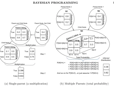
calculate the conditional distribution forX, all probability products of each combination leading to a given outcome are added together, as in Equation 2.7. This results in an N×1 matrix that is stored as a temporary posterior distribution estimate for P(X) which avoids frequent recalculation for determining the conditional distributions of children Ch(X) while traversing the network. This process is graphically illustrated in Figure 1 for a set of single parents (a) and for multiple parents (b).

In this way, any node in a Bayesian network can be queried to obtain a probability distribution over its values. While exact inference as described into a Bayesian network is widely understood to be an NP-hard problem Wu and Butz, 2005, it is still much more efficient than the raw computation of a joint distribution, and provides an intuitive, graphical method of representing dependencies and independences. It is easy to see how any system that can be described as a set of independent but conditional random variables can be abstracted into a Bayesian network, and that a wealth of information regarding the probability distributions therein can be extracted relatively efficiently.

3. Bayesian Programming

A Bayesian program has been defined by Lebeltel et al. as a group of probability dis-tributions selected so as to allow control of a robot to perform tasks related to those distributions. A “Program” is constructed from a “Question” that is posed to a “De-scription”. The “Description” in turn includes both “Data” represented byδ, and “Pre-liminary Knowledge represented by π. This “Preliminary Knowledge π consists of the pertinent random variables, their joint decomposition by the chain rule, and “Forms” representing the actual form of the distribution over a specific random variable, which can either be parametric forms such as Gaussian distributions with a given mean and standard deviation, or programs for obtaining the distribution based on inputs Lebeltel et al., 2000.

It is assumed that the random variables used such as X are discrete with a count-able number of values, and that a logical proposition of random varicount-ables [X = xi] is

mutually exclusive such that ∀i 6= j,¬(X = xi ∧X = xj) and exhaustive such that ∃X,(X =xi). All propositions represented by the random variable follow the

Conjunc-tion rule P(X, Y|π) = P(X|π)P(Y|X, π), the Normalization ruleP

XP(X|π) = 1, and

the Marginalization rule P

XP(X, Y|π) = P(Y|π) Bessiere et al., 2000. Rather than

unstructured groups of variables, we apply these concepts to a Bayesian network of M random variables℘=X1, X2, . . . , XN ∈π, δ, from which an arbitrary joint distribution

can be computed using conjunctions. It is assumed that any conditional independence of random variables inπandδ(which must exist, though it was not explicitly mentioned by Lebeltel et al.) is represented appropriately by the Bayesian network, thus significantly simplifying the process of factorization for joint distributions. The general process we use for Bayesian programming, including changes from the original BRP, is as follows:

(a) Define the set of relevant variables. This involves identifying the random variables that are directly relevant to the program desired. In a Bayesian network, this is implicit in the edges between nodes that represent dependencies. Usually, a single child node is queried to include information from all related nodes.

(b) Decompose the joint distribution. The original BRP methodology explicitly partitioned a joint distribution ofM variables P(X1, . . . , XM|δ, π) into subsets, each one

(a) Single-parent (a multiplication) (b) Multiple Parents (total probability)

Figure 1.Matrix calculations for querying a discrete random variable

the factorization rules in Equation 2.5 to reduce P(X1, . . . , XM|δ, π) to a product of

conditional distributions which are queried recursively P(X)

M

Y

m=1

P(Xm|δ, π). (3.1)

(c) Define the forms.For actual computations, the joint and dependent distributions must be numerically defined, which is done by inserting discrete values into each node. The most common function to be used, and the function used for continuous distributions in this work, is the Gaussian distribution with parameters mean ¯xand standard deviation σthat define the shape of the distribution, commonly formulated as

P(X=x) = 1 σ√2πe

−(x−x¯)2

2σ2 . (3.2)

A uniform distribution can also be set with P(X =x) =k, having the same probability regardless of value. Finally, because continuous distributions are programmed as function calls, a distribution that is a function into some arbitrary external process such as a map can be used.

Embedded Bayesian Network Robot Programming Methods 6

be used to determine the “final” answer to the question, namely a specific probability value in this distribution, we will generally use marginal MAP queries to obtain the value of highest probability taking into account the dependencies inU n, making the form of the question

arg max

Se

X

U n

P(Se, U n|Kn, δ, π). (3.3) The use of a Bayesian network formalizes the relationships of these sets, so that a query into a common child node ofSeincorporates information from parentsKnandU nofSe. It is important to note that a “question” is functionally another conditional distribution, and therefore operates in the same way as an additional node in the Bayesian network.

(e) Perform Bayesian inference. To perform inference into the joint distribution P(X1, . . . , XM|δ, π), the “Question” that has been formulated as a conjunction of the

three sets Searched (Se), Known (Kn), and Unknown (U n) is posed to the system and solved as a Bayesian inference that includes all relevant information to the set Se. For our Bayesian network implementation. The “Answer” is obtained as a probability distribution, and a specific maximum or minimum value can be obtained using a value from the setSeand a Maximum A Posteriori (MAP) query as

MAP(X|Y =y) = arg max

x

X

Z

P(X∩Z|Y). (3.4)

The last step in Bayesian programming is the actual inference operation used to deter-mine the probability distribution for the variable or set of variables in question. Obtaining the joint distribution P(Se|Kn, π) is the goal, and requires information from all related random variables in{Kn, U n, π}, which in the Bayesian network are visualized as parents ofSe. This distribution can always be obtained using Lebeltel and Bessi`ere, 2008

P(Se|Kn, δ, π) = 1 Σ

X

U n

P(Se, U n, Kn|δ, π) (3.5) where Σ =P

{Se,U n}P(Se, U n, Kn|δ, π) acts as a Normalization term. To complete the

inference calculation, we only need to reduce the distribution P

U nP(Se, U n, Kn|δ, π)

into marginally independent factors that can be determined. We assume that indepen-dence is denoted by the structure of the Bayesian network, so we only need be concerned with the ancestors of Se and do not need to scale by Σ. Given that inference into a Bayesian network typically involves querying a single node, we will assume thatSeis the singletonSe={X}. This can also be accomplished ifSeis larger by makingX a parent of all nodes inSe.

Applying the chain rule again to Bayesian networks, we can walk the Bayesian network backwards through the directed edges fromX, determining the conditional distribution of each node from its parents as we go, and therefore breaking down the determination of the joint distribution into smaller, separate calculations. ConsideringZto be the parents of each ancestor nodeY and following the method of Equations 2.6, and Equation 2.7, and Equation 3.5, a general expression for the factorization of P(Se|Kn, δ, π) through the Bayesian network is

P(Se|Kn, δ, π) = X

Y∈{X,An(X)



 Y

Z∈Pa(Y)

P(Y|Z)P(Z)



4. Bayesian Network Implementation

For our Bayesian network implementation, with the random variables inSe,Kn, andU n internally linked together as nodes and edges. Nodes associated with actions to be taken typically have conditional distributions that act as “questions” regarding their opera-tional state. If for example, the question is asked what should the right-side motors do?, the network nodes related to obstacle presence and mapping, and in turn, prior sensor data, will have to be traversed to obtain the Answer, which is a posterior probability distribution that is used to select a particular value of motor speed. Unlike most Bayesian network implementations, our implementation is unique in that it uses fixed-point math for storage and calculation and is programmed in C for better portability and calculation efficiency on small-scale embedded systems that do not have a floating-point arithmetic unit Lauha, 2006.

At minimum, a random variable withN possible values will have a 1×N distribution matrix. A parent node withM values will create at mostM additional distributions, and in general, if each parent has a distributionNl values in size, and there are L parents,

then the number of distributionsM possible in the child node areM =QL

l=1Nl, so the

storage size of the node scales roughly asNL_{. This can be mitigated to make processing}

more efficient by designing a deeper graph with more nodes and less parents per node. A parent node with anMl×Nldistribution matrix, regardless of the number of parents

and the size ofMl, will still only contributeNlvalues to its child nodes. A given nodeX

will then have to store a table of size|V(X∪Pa(X))|. Total probability requires that all values in each rowmsum to 1. The joint distribution P of probability values associated with a given random variable is the content actually stored.

Because the dimensionality of data stored in the node changes with number of parents, we use a single array for storing the distribution and index it with a linear index that is a function of the parent numbers of the node. To create the index, we model the array as an L+ 1-dimensional matrix forL parents and calculate an indexi. For a two-dimensional row-major-order matrix with row (m) and column (n) indices, i = n+m∗columns. By recognizing that each additional dimension must be indexed by multiplying past the sizes of all preceding dimensions, we can set index i using matrix indices m1 for

dimension 1 of sizeM1(we choose columns here for consistency),m2 for dimension 2 of

size M1(we choose rows here for consistency), andm3, m4, . . .and above for additional

matrix dimensions of sizeM3, M4, . . .respectively, obtaining

i=m1+m2M1+m3M2M1+. . .+mL+1 L

Y

l=1

Ml= L+1

X

n=1

mn n−1

Y

l=1

Ml

!

. (4.1)

5. Sensory Reasoning Example

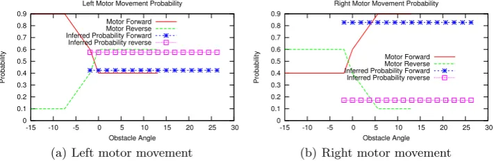
To test the concepts and implementation detailed above, a simple six-node network was set up which is graphed with base probabilities as shown in Figure 2, consisting of three nodes representing obstacle sensors with states{Clear, Obstacle}angled 30 degrees apart in front of a mobile robot, a sensor fusion node that uses Gaussian distributions to estimate the detection angles of the three sensors, and two motor nodes for control of left and right side motors. A MAP query is used to determine the most appropriate state of the motors from{F orward, Reverse} given inference into the sensor data.

Embedded Bayesian Network Robot Programming Methods 8

LeftSensor ~0.800, 0.200,

FusedSensor

~0.003, 0.006, 0.010, 0.016, 0.022, 0.027, 0.030, 0.031, 0.030, 0.027, 0.024, 0.022, 0.022, 0.021, 0.018, 0.014, MiddleSensor ~0.800, 0.200, RightSensor ~0.800, 0.200, LeftMotor ~0.600, 0.400, RightMotor ~0.600, 0.400,

Figure 2.Simple Bayesian Network for Obstacle Avoidance Program

0 0.02 0.04 0.06 0.08 0.1 0.12 0.14

-15 -10 -5 0 5 10 15

Probability

Obstacle Angle Angular Probability

Obstacle to Left Obstacle Mid Left Obstacle in Middle Obstacle Mid Right Obstacle to Right Inferred Distribution

(a) No obstacles detected

0 0.02 0.04 0.06 0.08 0.1 0.12 0.14

-15 -10 -5 0 5 10 15

Probability

Obstacle Angle Angular Probability

Obstacle to Left Obstacle Mid Left Obstacle in Middle Obstacle Mid Right Obstacle to Right Inferred Distribution

(b) Obstacle detected to right (90%)

Figure 3.Sensor Fusion Probability Priors and resulting Inferred Distributions

0 0.1 0.2 0.3 0.4 0.5 0.6 0.7 0.8 0.9

-15 -10 -5 0 5 10 15 20 25 30

Probability

Obstacle Angle Left Motor Movement Probability

Motor Forward Motor Reverse Inferred Probability Forward Inferred Probability reverse

(a) Left motor movement

0 0.1 0.2 0.3 0.4 0.5 0.6 0.7 0.8 0.9

-15 -10 -5 0 5 10 15 20 25 30

Probability

Obstacle Angle Right Motor Movement Probability

Motor Forward Motor Reverse Inferred Probability Forward Inferred Probability reverse

(b) Right motor movement

Figure 4.Priors for Motor Movement and Probabilities of Obstacle Avoidance for Obstacle Detected to Right (90%)

sensor actually detects an obstacle. The sensor fusion node is pre-loaded with a set of six Gaussian functions representing an approximate likelihood of the direction of an obstacle given the six possible states of the three two-state obstacle sensors. Figure 3 shows the angular probabilities of these Gaussian functions and the resulting inferred distribution (denoted with markers) for (a) no obstacles detected, and (b) an obstacle detected by the right-hand sensor with 90% probability.

The motor nodes are defined with a high probability of reverse movement for obstacles detected on the opposite side to cause obstacle avoidance behaviour, but generally a higher probability of forward movement to keep the robot moving forward if obstacles are unlikely. The functions used are shown in Figure 4 for the right and left motors

“prob-ability” of the left motor reversing, which in this context would be contextualized as “probability that reversing will avoid an obstacle”, and the motor will reverse when a MAP query is applied. Optimal priors can be determined by expert knowledge or by statistical learning methods which will be a focus of future work. Graphing the priors used for inference at each node shows a notable similarity to fuzzy functions, and the process of inference into discrete values that of fuzzification, but there are still fundamen-tal differences. A random variable is expected to have a single outcome while fuzzy sets represent multiple outcomes, or alternately imprecise degrees of belief. This imprecision is reflected in the extension to fuzzy sets of possibility theory, which can be seen as a form of upper probability theory Zadeh, 1999.

6. Conclusions

We have described a method for making decisions using the Bayesian Robot Programming paradigm using Bayesian networks for organization of data and efficient algorithms for storage and inference into discrete random variables. This method has been implemented as a novel, efficient, structured framework for practical use of Bayesian networks and probabilistic queries on an embedded system with fixed-point arithmetic, leading to an efficient and intuitive way of representing robotic knowledge and drawing conclusions based on statistical information encapsulated in the network.

The applicability of these methods to robotic programming and control is very wide, and many future applications are expected, as this method can be extended to much more complex systems simply by adding networked random variables for sensor and actuator quantities, so long as they can be probabilistically characterized. Future work includes implementations for new applications, determination of network structure and optimal priors from existing hardware data, and the implementation of statistical learning methods to improve performance of the system while it operates.

REFERENCES

Bessiere, P., Lebeltel, O., Lebeltel, O., Diard, J., Diard, J., Mazer, E., and Mazer, E. (2000). Bayesian robots programming. InResearch Report 1, Les Cahiers du Laboratoire Leibniz, Grenoble (FR, pages 49–79.

Engelbrecht, A. P. (2002). Computational Intelligence: An Introduction. John Wiley & Sons. Kjrulff, U. B. (2008).Bayesian Networks and Influence Diagrams: A Guide to Construction and

Analysis. Springer Science.

Koller, D. and Friedman, N. (2009).Probabilistic Graphical Models, Principles and Techniques. MIT Press, Cambridge, Massachusetts.

Lauha, J. (2006). The neglected art of fixed point arithmetic. Presentation.

Lebeltel, O. and Bessi`ere, P. (2008). Basic Concepts of Bayesian Programming. InProbabilistic Reasoning and Decision Making in Sensory-Motor Systems, pages 19–48. Springer. Lebeltel, O., Bessi`ere, P., Diard, J., and Mazer, E. (2004). Bayesian robot programming.

Au-tonomous Robots, 16(1):49–79.

Lebeltel, O., Diard, J., Bessiere, P., and Mazer, E. (2000). A bayesian framework for robotic programming. InTwentieth International Workshop on Bayesian Inference and Maximum Entropy Methods in Science and Engineering (MaxEnt 2000), Paris, France.

Post, M. (2014).Planetary Micro-Rovers with Bayesian Autonomy. PhD thesis, York University. Wu, D. and Butz, C. (2005). On the complexity of probabilistic inference in singly connected bayesian networks. In Slezak, D., Wang, G., Szczuka, M., Dntsch, I., and Yao, Y., editors, Rough Sets, Fuzzy Sets, Data Mining, and Granular Computing, volume 3641 of Lecture Notes in Computer Science, pages 581–590. Springer Berlin Heidelberg.