Predicting fatigue damage in composites : a Bayesian framework

Predicting Fatigue Damage in Composites: A Bayesian Framework

Manuel Chiach´ıoa,∗, Juan Chiach´ıoa, Guillermo Rusa, James L. Beckb

a_{Dept. Structural Mechanics and Hydraulic Engineering, University of Granada.}

Campus de Fuentenueva s/n, 18071 Granada, Spain.

b_{Division of Engineering and Applied Science, 9-94, California Institute of Technology, Pasadena, CA}

91125, USA.

Abstract

Modeling the progression of damage in composites materials is a challenge mainly due to

the uncertainty in the multi-scale physics of the damage process and the large variability

in behavior that is observed, even for tests of nominally identical specimens. As a result,

there is much uncertainty related to the choice of the class of models among a set of possible

candidates for predicting damage behavior. In this paper, a Bayesian prediction approach

is presented to give a general way to incorporate modeling uncertainties for inference about

the damage process. The overall procedure is demonstrated by an example with test data

consisting of the evolution of damage in glass-fiber composite coupons subject to

tension-tension fatigue loads. Results are presented for the posterior information about the model

parameters together with the uncertainty associated with the model choice from a set of

plausible fatigue models. This approach confers an efficient way to make inference for damage

evolution using an optimum set of model parameters and, in general, to treat cumulative

damage processes in composites in a robust sense.

Keywords: FRP composites, fatigue, Markov chains, Bayesian inverse problem, model

class selection

∗_{Corresponding author. e-mail: [email protected]}

1. Introduction

In composite materials, fatigue damage represents one of the most important sources of

uncertainty for in-service behavior. This leads to conservative designs and higher costs in

manufacture and maintenance [1]. Throughout decades of investigation, numerous fatigue

models have been proposed [2–5] and a large amount of data has been derived from expensive

experimental programs. The vast majority of these models are deterministic semi-empirical

formulations calibrated for a particular material configuration under some specific testing

conditions. Therefore, they not only neglect the modeling uncertainty coming from the

adoption of a single value for model parameters, but also from the selection of a particular

model class (e.g., the parameterized mathematical structure of the model for the damage

behavior).

Some researchers have addressed uncertainty in fatigue modeling using Bayesian

meth-ods, mostly focused on crack propagation in metals [6–11]. However the application of a full

Bayesian inverse-problem framework for assessing the modeling uncertainty still remains

very limited for the study of the fatigue degradation of composite materials, precisely where

the benefits of this framework can be fully exploited to deal with the well-known uncertainty

of the fatigue damage process.

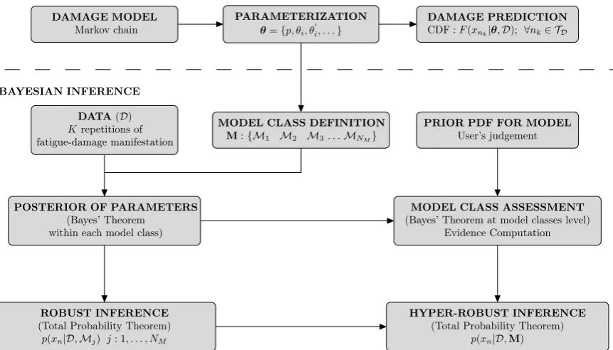
In this work, a full Bayesian prediction and updating framework is presented in

appli-cation to the problem of fatigue damage progression in composite materials. To this end,

Bayes’ Theorem is applied for two levels: first, to deal with the posterior information about

the model parameters for a specific model class, and second, to assess a degree of plausibility

of each model class within a candidate set of models [12]. Here, probability is interpreted

as a multi-valued logic that expresses the degree of plausibility of a proposition conditioned

on the given information, because this interpretation provides a rigorous foundation for the

Bayesian approach [13, 14]. Consequently, the approach has the advantage of being able

to quantify the uncertainties associated with (1) model parameters and (2) model choice

for the damage behavior, and then to further make robust response predictions of fatigue

provides a conceptual scheme of the proposed Bayesian framework for damage prediction.

A cumulative damage model based on the theory of Markov chains [15] is used to infer a

complete damage process from batch sequences of damage data. The proposed framework is

not limited to this model choice, but Markov chains damage models [16] are of major interest

due to their versatility and efficiency. Markov chains were first applied to fatigue modeling

in composites by Rowatt et al. [17] as an extension of the pioneering work of Bogdanoff et

al. [16]. Other relevant examples of Markov chains models for fatigue in composites are

found in [18–21] while for metals in [22–28]. More applications and theoretical insight about

stochastic cumulative damage models are provided in [29–31]. As a novelty, a new model

parameterization is introduced to account for the nonstationarity based on a generalization

of the time transformation-condensation method first developed by Bogdanoff et al. [16].

As an example, the full Bayesian framework is applied to damage data for sixteen

quasi-isotropic open-hole S2-glass laminates subject to constant amplitude tension-tension fatigue

loading. The results show that accounting for the underlying uncertainty in stochastic fatigue

models allows one to obtain a more robust data-based model of the fatigue process, in the

sense of a trade-off between data fitting and model complexity to avoid the extremes of

over-fitting or under-fitting the data. For the same reason, this framework can be used to

select a parsimonious number of parameters to represent the fatigue process degradation

within the context of the stochastic model presented in this work.

Section 2 of this paper is devoted to providing the basis and main assumptions about the

proposed Markov chain damage model and also to defining the stochastic model classes to

be considered. In Section 3, the problem of inference of a Markov chain model is formulated

using a Bayesian inverse problem framework. This section also gives the basis of Bayesian

model class selection and the corresponding computational issues that must be addressed

for our needs. In Section 4, our framework is applied to a set of fatigue data to serve as an

2. Forward prediction problem

2.1. Markov chain forward model

The starting point of our fatigue modeling approach is to model the evolution of

fa-tigue damage as a discrete-state Markov chain [15]. This approach models the damage as

a nondecreasing stochastic process _{xn, n ∈ N} taking values in X = [0,1] ⊂ R, where

xn at fatigue cycle n is the macroscopic relative stiffness reduction at one specific point,

section or element [32, 33]. Damage passes monotonically through a finite set of damage

states, _Xi ⊂ X where i ∈ I = {0, . . . , s} ⊂ N, until the “absorbing” state Xs is reached

[16]. The no-damage state corresponds to i= 0. Each damage state _Xi ⊂ X is a subinterval

represented by its center ¯xi_n=2i+ 1_{/2s+ 2 such that p}i

n, p(¯xin),P [xn ∈ Xi]>0. Once the damage at cycle n is at a certain state ¯xi

n, it may go only to the next state in one cycle ¯

xi_n+1₊₁ with probability pi,i_n+1 _, p(¯xi_n+1_+1|x¯i_n), and remain in the same state with probability

pi,i

n ,p(¯xin+1|x¯in) = 1−pi,in+1. Additionally, this approach assumes that the set of load cycles is divided into N disjoint subsets or “duty cycles” (DC), _T = _{1, . . . , n, . . . , N_{} ⊂ N}, in

which damage can be accumulated.

From the last remarks it follows that the damage at a certain DC n is entirely defined

by means of the probabilities of all possible damage states _{x¯0

n,x¯1n. . . ,x¯sn}, summarized by the probability mass function (PMF) pn = [p0n, p1n, . . . , psn]. By Markov chain theory, the

probability of damage at DCn+ 1 can be obtained as

pn+1 =pn·Pn (1)

with Pn the “one-step” probability transition matrix for DCn [16], and for generalm > n,

pm =pn· m−1

Y

j=n

Pj (2)

For a certain DCn, the matrixPnstores in its (i+1, j+1) element the conditional probability

of transition p(¯xj_n+1|x¯i

n) = pi,jn from state ¯xin to ¯x j

restricts the structure of Pn to a bi-diagonal (s+ 1)×(s+ 1) matrix with ps,sn = 1, then:

Pn =       

p0n,0 p0n,1

p1n,1 p1n,2

... ...

psn−1,s−1 psn−1,s

1        (3) where

pi,i_n +pi,i_n+1 = 1; i_{∈ {}0, . . . , s₋1_} (4)

If the transition probabilities pi,j

n do not depend on the duty cycle n, then Pn =P ∀n ∈

N and the process is termed stationary. Otherwise, in the more general case where the

transition probabilities may change with time (i.e. with load cycles), the process is

non-stationary. More details about Markov chain models of cumulative damage are given in [16].

2.2. Parameterization for non-stationarity

For the purpose of inference, a parameterization strategy is needed to avoid a high

dimensional problem for characterizing the non-stationary Markov chain model described

above. The strategy consists of adopting the same value of the one-step probability of

tran-sition along the process for every statei _{∈ {}0, . . . , s₋1_}, except for the absorbing state in

which ps,s

n = 1. This allows us to have a single probability transition matrix, now called Q, that remains invariant during the process, defined as:

Q=     

1−p p

1−p p ... ...

1−p p

1      (5)

To account for the non-stationarity, anad-hoc modification of the “natural” time scale n

into a transformed time scale n0 =g0(n) is introduced such that any probability transition matrix from stepn to stepm can be calculated asQg0(m)−g0(n), satisfying:

m−1

Y

j=n

Pj =Qg

0_(m)−g0_(n)

where g0(n) is a nonlinear function of n, that is given below. This procedure is based on the time transformation-condensation method (TTCM) first proposed by Bogdanoff and

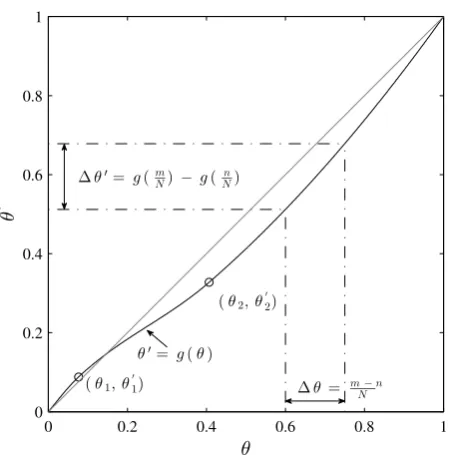
Kozin [16] by using undefined polynomials. Instead, we expressg0(n) in terms of a continuous monotonic functiong(θ) : [0,1]_→[0,1] as follows:

g0(n) = N_· g(n_{/N) (7)}

where the functiong is suitably defined as an interpolating monotonic cubic spline [34] for a

given set ofj _∈Ninterpolation points_{θ1, θ 0

1, . . . , θj, θ 0

j}andN is a sufficiently large amount of duty cycles along which damage is completely developed. In this work,N is chosen as the

maximum length of the observed damage sequences. Notice also that to maintain the matrix

structure of the model, the exponent g0(m)₋g0(n) in Equation 6 must be an integer after the transformation, to which an approximation to the nearest integer is applied, otherwise

a condensation technique as proposed in [16] must be considered.

The transformation in Equation 7 distorts the natural time scale by using a nonlinear

mapping over the unit interval, which has the double benefit over the TTCM of (1) having a

bounded and defined searching space, and (2) keeping a fixed number of parameters. Figure

2 illustrates this concept. Each interpolation point is defined by its cartesian coordinates

[θj, θ

0

j] in the unit time scale, and together with p, act as model parameters for the Markov chain model that allows for a complete description of the fatigue damage process. Then the

Markov chain damage model can be reformulated by replacing Equation 2 with:

pm =pn·Qg

0_(m)−g0_(n)

(8)

2.3. Model class definition

We denote by _Mj the jth Bayesian model class [12] that incorporates the Markov chain

forward model with θj = {θ1, θ 0

1, . . . , θj, θ

0

j, p} ∈ Θj as model parameters along with the prior PDF p(θj|Mj), that gives the initial relative plausibility of each value of θj before

the information from measurements is incorporated. Henceforth, we drop the subscript j

on θ since conditioning on _Mj is sufficient to indicate which parameter vector is being

M = _{Mj, j : 1,2, . . . , NM}, NM ∈ N, is obtained. See Table 1 for a summary of the

parameterization of the set of model classes M.

3. Bayesian inverse problem

A rigorous foundation for the Bayesian approach to inverse problems is given by the

Cox-Jaynes theory of probability as a multi-valued logic for plausible inference [14, 35, 36]. The

focus in Bayesian inversion [37] is to investigate the posterior probability density function

of the model parameters θ over the set Θ_⊂Rd of possible values, which is given by Bayes’

Theorem. This PDF is interpreted as a measure of the relative plausibility of the values

of θ conditional on the available information. It is a measure of the uncertainty about the

parameter values and not an inherent property of the real system. The available information

is based on a set of data _D from measurements on the system together with any relevant

prior information that can be utilized.

We denote the likelihood function for model class _Mj ∈ M by p(D|θ,Mj). It provides

a measure of how well the model specified by θ predicts the actual data _D. It is given by

the PDF defined by the stochastic forward model parameterized by θ when it is evaluated

at data_D. Bayes’ Theorem gives the posterior PDF p(θ_|D,_Mj) for the model specified by

θ in the class _Mj, as:

p(θ_|D,_Mj) = c−1p(D|θ,Mj)p(θ|Mj) (9)

wherec is a normalizing constant, so that:

Z

Θ

p(θ|D,_Mj)dθ =c−1 Z

Θ

p(_D|θ,_Mj)p(θ|Mj)dθ= 1 (10)

Notice that Bayes’ Theorem takes the initial quantification of the plausibility of each model

specified byθin the model class_Mj, which is expressed by the prior probability distribution,

and updates this plausibility by using the information in the data _D expressed through the

likelihood function. Note also that the normalizing constant c in Bayes’ Theorem does not

affect the shape of the posterior distribution. The difficulty in applying Bayes’ Theorem

integration methods, if the dimension d is not small. However, stochastic simulation based

on MCMC methods can be used to obtain samples from the posterior without knowingc in

Equation 9, as done in Section 3.2.

3.1. Formulation of the likelihood function

In our problem, data _D consist of a set of K experimental sequences of fatigue-based

damage fromKnominally-identical specimens,Yˆ =_{Yˆ(1)_{, . . . ,Yˆ}(k)_{, . . . ,Yˆ}(K)_{}where ˆY}(k)₌

h ˆ y(nk1),yˆ

(k)

n2 , . . . ,yˆ

(k)

nN i

, is the measured relative stiffness reduction at a discrete set of

reg-ularly scheduled or even opportunistically staggered duty cycles _TD = {n1, n2, . . . , nN}, such that _TD ⊆ T. A correspondence between the observed damage sequence ˆY(k) =

h ˆ y(nk1),yˆ

(k)

n2 , . . . ,yˆ

(k)

nN i

and the latent sequence of damage states hx¯i,n(1k),x¯

j,(k)

n2 , . . . ,x¯

l,(k)

nN i

, with

i, j . . . , l_∈I, can be established based on the defined set _{x¯0_n,x¯1_n, . . . ,x¯s_n} in Section 2.1, by

taking ¯xi,n(k) when ˆy(nk) ∈ Xi. See Figure 3 for further details.

The likelihood function can be formulated as follows. First, the probability to observe

a sequence of damage states _{x¯i,n1(k),x¯

j,(k)

n2 , . . . ,x¯

l,(k)

nN } in the k

th _{specimen at the given set of}

duty cycles_TD ={n1, n2,. . . , nN},TD ⊆ T, is modeled as a Markov chain parameterized by

θ. By means of the Markov property, this probability can be obtained as follows:

p(¯xi_n1,x¯j_n2, . . . ,x¯_nl_N|θ) = p(¯xi_n1|θ)p(¯xj_n2|x¯i_n1,θ)_{· · ·}p(¯xl_nN|x¯k_nN−1,θ) (11)

where the superscript (k) denoting the kth _{specimen is not used in the last equation, and}

furthermore, the conditioning on the model class_Mj is omitted. The likelihood function is

then the product of probabilities as in Equation 11 over all K specimen test sequences.

The structure of this likelihood function can be clarified by introducing the matrix fnh,

called the transition count matrix, that accounts for the number of observed transitions

¯ xi

nh →x¯ j

nh+1, i.e., the number of times for which the damage reaches the statej at DCnh+1,

given that it previously was in state i at DC nh [38, 39]. In mathematical terms, the (i, j)

element of this matrix can be expressed as:

f_ni,j h = K X k=1 s X

i∗_,j∗₌₀ I

¯ xi_n∗=i,(k)

h ,x¯ j∗=j,(k)

nh+1

with i∗, j∗ = 0, . . . , s _∈ I and ¯xni(hk) the damage state i at duty cycle nh, for the k

th

speci-men. In the last expression, _Ix¯ni∗h=i,(k),x¯ j∗=j,(k)

nh+1

is an indicator function which assigns the

value of 1 when the transition ¯xi

nh → x¯ j

nh+1 holds, and 0 otherwise. See Figure 3 for a

de-tailed example about the construction offnh considering two hypothetical curves of stiffness

reduction from two specimens. The likelihood function can then be formulated as:

p(_D|θ,_Mj) =p(¯xin1|θ)

nN−1

Y

nh=n1

s Y

i,j=0

p(¯xj_nh+1|x¯i_nh,θ) f_nhi,j

(13)

wherep(¯xj nh+1|x¯

i

nh,θ) is the probability transition between damage statesi and j at DC nh andnh+1 respectively, corresponding to the (i+1, j+1) element of the matrixQg

0_(n

h+1)−g0(nh)_, which is obtained by the model parameterizationθ _{∈ M}j.

Finally, we remark that in constructing the likelihood function in Equation 13, any

measurement error when assigning theith damage state based on the observed value ˆyn∈ Xi

at duty cyclenis subsumed by the uncertainty in the damage states described by the Markov

chain model, and so it is not explicitly modeled.

3.2. Stochastic simulation

The goal of stochastic simulation methods in Bayesian updating is to generate

sam-ples which are distributed according to the posterior probability density function (PDF)

in Equation 9. For this task, several algorithms have been proposed in the literature such

as the Metropolis-Hastings, Gibbs Sampler and Hybrid Monte Carlo algorithms. A recent

comprehensive overview of MCMC algorithms is given by Lianget al. [40].

Among them, the Metropolis-Hastings (M-H) algorithm is widely used for its versatility

and implementation simplicity [41, 42]. This algorithm generates samples from a specially

constructed Markov chain whose stationary distribution is any specified target PDF, known

up to a scaling constant. By sampling a candidate vector θ0 from a proposal distribution q(θ0_|θ), the M-H algorithm obtains the state of the chain at ζ + 1, given the state at ζ,

specified byθ(ζ). The candidateθ0 is accepted as the next state of the chain with probability min _{1, r_}, where:

r = p(θ

0

|D,_M)q(θ(ζ)

|θ0) p(θ(ζ)

Ifθ0 is rejected, the previous state is repeated,θ(ζ+1) _=θ(ζ)_.

An important consideration is the specification of the variance σ2_q for the proposal

dis-tribution, which has a significant impact on the speed of convergence of the algorithm

[42]. Small values tend to produce candidate samples that are accepted with high

probabili-ties, but may result in highly dependent chains that explore the state space very slowly. In

contrast, large values of σ2_q tend to produce large steps in state space, but result in small

acceptance rates 1_{. Thus, it is often worthwhile to select appropriate proposal variances by}

controlling the acceptance rates in a certain range, depending on the dimension d of the

proposal PDF, via some pilot runs [43, 44]. The interval [20%₋40%] is suggested for the

acceptance rate in low dimensional spaces, say d₆10, as in our case.

3.3. Model-class assessment

Following the model class definition given in Section 2.3, different model classes can be

formulated and hypothesized to idealize the experimental system, and the previous Bayesian

theory can be applied to each of them. Then, to select among a set of candidate model classes

M=_{Mj, j= 1, . . . , NM}, a rigorous procedure is used to Bayesian model class assessment

that judges the relative plausibility of each candidate model class based on their probabilities

p(_Mj|D,M) conditional on data [12, 45, 46], where the probabilities can be obtained by

Bayes’ Theorem at the model class level:

p(_Mj|D,M) =

p(_D|Mj)p(Mj|M)

XNM

i=1p(D|Mi)p(Mi|M)

(15)

In the last equation, p(_Mj|M) is the prior probability of each Mj, that expresses the

user’s judgement on the initial relative plausibility of_Mj. The factor p(D|Mj) is called the

evidence (or marginal likelihood) for the model class _Mj provided by the observed data

D. It expresses how likely these data are according to the model class _Mj, and it can be obtained as follows:

p(_D|Mj) = Z

Θ

p(_D|θ,_Mj)p(θ|Mj)dθ (16)

1_{Defined as the relation between the number of accepted samples over the total amount of candidate}

Notice also that the evidence is equal to the normalizing constant c in establishing the

posterior PDF in Equations 9 and 10.

Once the evidence p(_D|Mj) is computed for each model class, their values allow us to

rank the model classes according to how plausible they are based on observations. In certain

cases, more than one model class may have significant posterior probability in comparison

with the rest of the setM. Then, posterior model class averaging provides a coherent

mech-anism to account all these model classes for response prediction [12, 45, 47], as is shown in

Section 4.

3.3.1. Interpretation of model class evidence

From the perspective of forward modeling problems, more complex models may be

pre-ferred over simpler models because they are considered more realistic. For inverse problems,

however, this may lead to over-fitting of the data where the model is unnecessarily adjusted

to fit the specific set of data used. Then the model does not generalize well when

mak-ing predictions. The Bayesian approach to model class assessment shows that the posterior

probability of each model class (or directly the evidence when p(_Mj|M) =1/NM)

automat-ically enforces a quantitative expression of a Principle of Model Parsimony or Ockham’s

razor [14, 48], by which simpler models that are reasonably consistent with data should be

preferred over more complex models that lead to only slightly better agreement with the

data. In the case of globally identifiable model classes [49, 50] based on the data, the

pos-terior PDF in Equation 9 may be accurately approximated by a Gaussian distribution, and

the evidence term can be obtained by Laplace’s approximation [46, 49, 51].

In the more general case where the posterior PDF may not be approximated well by a

Gaussian distribution, Muto and Beck [52] proposed an information theoretic point of view

for the interpretation of the evidence for a model class, as follows:

logp(_D|Mj) = Z

Θ

[logp(_D|θ,_Mj)]p(θ|D,Mj)dθ− Z

Θ

log p(θ|D,Mj) p(θ|Mj)

p(θ|D,_Mj)dθ

(17)

factor of one:

logp(_D|Mj) = logp(D|Mj)

Z

Θ

p(θ|D,_Mj)dθ

| {z }

= 1

(18)

and then making substitutions according to Bayes’ Theorem in Equation 9 to expand the

evidence.

The first term of the right side of Equation 17 is the posterior mean of the

log-likeli-hood function, which is a measure of the average goodness of fit of the model class _Mj

to the data _D. It accounts for the goodness of fit for different combinations of the model

parameters, weighted by their posterior probabilities [12, 52]. The second term is the relative

entropy between the posterior and prior PDF of the model parameters. It can be interpreted

as the expected information gain [EIG] about the model parameters from the data _D and

it will usually be larger for more complex models with more parameters. Applying

Equa-tion 15 therefore provides an automatic trade-off between model simplicity and fitting to

observations, which explicitly reveals a quantitative Ockham’s razor [12].

3.3.2. Computation of the evidence for a model class

The calculation of the evidence given in Equation 16 is not a trivial task. If the conditions

cited in the last section for analytically approximating the posterior do not apply, or if

the amount of data is small [46], then stochastic simulation methods are required. One

straight-forward way to approximate the evidence is by considering the probability integral

in Equation 16 as a mathematical expectation of the likelihood p(_D|θ,_Mj) with respect to

the prior p(θ|Mj). This approach leads to the direct Monte Carlo method as follows,

p(_D|Mj)≈ 1 N1

N1

X

k=1

p(_D|θ(k),_Mj) (19)

where theθ(k) are N1 samples drawn from the prior. Although this calculation can be easily

implemented, it results in a computationally inefficient method (large-variance estimator),

since the region of probability content of p(θ|Mj) is usually very different from the region

where the likelihood p(_D|θ,_Mj) has its largest values. To overcome this problem, some

have received attention, although with known drawbacks of instability [53]. In this paper,

a recent stable technique based on an analytical approximation of the posterior is used

[54]. The relevant details from [54] are presented here in a concise way with special focus on

the Metropolis-Hastings algorithm, which is the algorithm used in this work.

LetK(θ_|θ∗) be the transition PDF of any MCMC algorithm with stationary PDFπ(θ) = p(θ|D,_Mj). The stationarity condition for the MCMC algorithm satisfies the following

relation:

π(θ) = Z

K(θ|θ∗)π(θ∗)dθ∗ (20)

A general choice ofK(θ|θ∗) that applies to many MCMC algorithms, can be defined as:

K(θ_|θ∗) = T(θ_|θ∗) + (1₋a(θ∗))δ(θ₋θ∗) (21)

where T(θ|θ∗) is a smooth function that does not contain delta functions and a(θ∗) is the acceptance probability which must satisfy a(θ∗) = R

T(θ_|θ∗)dθ 6 1. By substituting Equation 21 into 20, an analytical approximation of the posterior results as follows:

π(θ) =p(θ_|D,_Mj) = R

T(θ|θ∗)π(θ∗)dθ∗

a(θ) ≈

1 a(θ)N1

N1

X

k=1

T(θ_|θ(k)_{) (22)}

where theθ(k) _{are N}

1 samples distributed according to the posterior. For the special case of

the Metropolis-Hastings algorithm,T(θ|θ∗) =r(θ|θ∗)q(θ|θ∗), whereq(θ|θ∗) is the proposal PDF, andr(θ_|θ∗) is given by:

r(θ_|θ∗) = min (

1, p(D|θ,Mj)p(θ|Mj)q(θ

∗

|θ) p(_D|θ∗,_Mj)p(θ∗|Mj)q(θ|θ∗)

)

(23)

Additionally, for this algorithm, the denominator in Equation 22 can be approximated by

an estimator that uses samples from the proposal distribution as follows:

a(θ) = Z

r(˜θ|θ)q(˜θ|θ)dθ˜≈ 1 N2

N2

X

k=1

r(˜θ(k)|θ) (24)

where the ˜θ(k) are N2 samples from q(˜θ|θ), when θ is fixed. Once the analytical

evidence,

logp(_D|Mj)≈logp(D|θ,Mj) + logp(θ|Mj)−logp(θ|D,Mj)

| {z }

Analytical approx.

(25)

Bayes’ Theorem ensures that the last equation is valid for all θ_∈Θ, so it is possible to use

only one value for this parameter. However a more accurate estimate for the log-evidence can

be obtained by averaging the results from Equation 25 using different values for θ [54]. In

this work, three different values of θ from the peak region of p(θ|D,_M) are employed for

the evidence calculation. Once the evidence is obtained, the data-fit term in Equation 17

can also be estimated based on the N1 samples from the posterior, and then the EIG term

in this equation can be approximated by:

E

log p(θ|D,Mj) p(θ|Mj)

≈ 1

N1

N1

X

k=1

logp(_D|θ(k),_Mj)−logp(D|Mj) (26)

4. Application of methodology to fatigue test data

To illustrate the proposed framework, a set of data taken from literature [20] is

se-lected. These data are based on experimental sequences of damage corresponding to sixteen

quasi-isotropic glass fiber notched laminates S2-Glass/E733FR, that were subjected to

iden-tical and independent tension fatigue tests. See Figure 4 for a graphical representation of

the damage series. The tests were conducted under load-controlled fatigue loadings with a

frequency of f = 5Hz, a maximum applied tension of 50% of their ultimate stress, and a

stress ratio R= 0.1 (relation between the minimum and maximum stress for each cycle).

Some pilot tests revealed that the most suitable value for duty cycle DC for these data

is 500 load cycles with a Markov chain assembly of s= 30 states. Hence, the total number

of duty cycles is N = 213900_{/500 = 428. In the experiment, some measurements were taken}

outside of the [0,1] interval because of experimental error in measuring stiffness. Hence, to

ensure the existence of an absorbent state for the stochastic process, it is re-defined as the

state corresponding to the first measurement that fulfills ¯xnh >1. This definition only affects

a small portion of measurements near the absorbent state where transition probabilities are

Four model classes are considered sufficient for the inference, so NM = 4. This implies

that a maximum of 9 parameters are employed for the modeling: from 3 parameters for_M1 to

9 for_M4(see Table 1). For each model class, the prior is chosen as the product of independent

uniform distributions2 for each model parameter, p(θi_|Mj) = U(0,1), i = 1, . . . , d, where

θ_∈Rd. Therefore the posterior is given by:

p(θ|D,_Mj) = c2p(D|θ,Mj) (27)

over the unit hypercube of dimension d and it is zero outside of it, where the likelihood

function is given by Equation 13. For all test specimens, we consider the fatigue process

starting from the no-damage state ¯x0_n1, so the probability p(¯x0_n1|θ) in Equation 13 is equal

to 1.

The M-H algorithm is applied with a multivariate Gaussian for the proposal PDF with

identical standard deviation in each dimension, which corresponds to theRandom Walk

ver-sion of the algorithm [55]. See the algorithm configuration in Table 2. CPU times of 1800 [s],

1800 [s], 1950 [s] and 2100 [s] are required on average to complete theN1 = 104 simulations

for model classes _M1 to M4 respectively, using a 2.6 GHz double-core system. Note from

Table 2 that the more parameters that are included in the model definition, the smaller the

value ofσq that is required to achieve an acceptance rate within the recommended interval

of [20%₋40%] for a given number of simulations, which agrees with [43, 44]. It is noted that

choosing the first sample of the θi and θ_i0 parameters with values close to the diagonal in Figure 2, reduces significantly the burn-in period and so the time to convergence.

Mathemat-ically: (θ1 ≈θ 0

1)<(θ2 ≈θ 0

2). . . <(θNM ≈θ

0

NM). In fact, this selection for the first sample is consistent with the non-stationarity of the fatigue processes of composite materials, where

degradation is not abrupt but gradual in time [56].

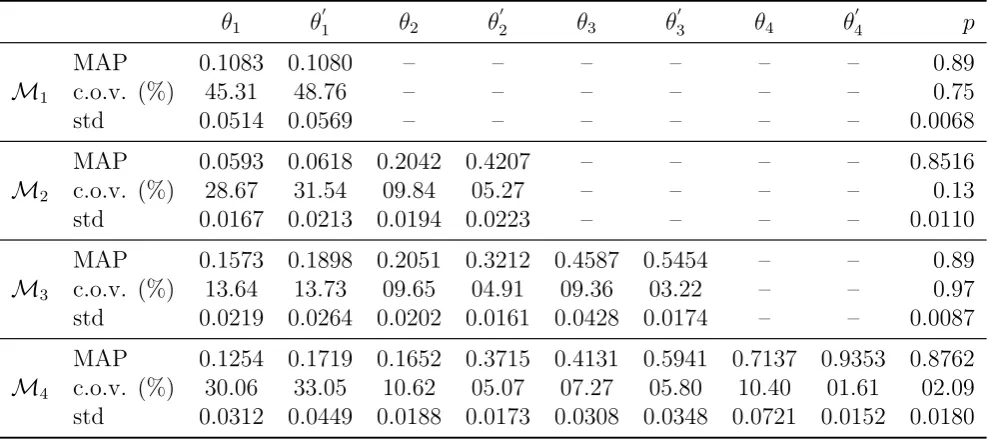
The posterior results for the parameters are summarized in Table 3 for models _M1 to

M4. In Figures 5 to 7, all two-dimensional projections of the posterior samples are plotted

2_{A rational way to define a probability model for the prior PDF is to select it such that it produces the}

largest uncertainty (largest Shannon entropy) [14, 36]. The maximum-entropy PDF for a bounded variable

for model classes _M1 toM3, respectively. The plot for model class M4 is avoided because

its contribution to the inference is negligible and the required space for printing purposes

is high. Observing the posterior information for model _M1 in Figure 5, it is noted that

θ1 and θ 0

1 are highly correlated along the straight line from (0,0) to (1,1), but they are

practically uncorrelated withp, which has a narrow range of plausible values between about

0.87 and 0.92. This means that given our data_D, model_M1 will produce stochastic damage

predictions very close to a stationary model, where the transition probability p is the only

model parameter.

4.1. Assessment of model classes

In order to choose which model class or set of model classes are more plausible based on

data_D, the results in Table 3 are not enough. In accordance with the theory in Section 3.3,

the best choice among model classes will be those with the higher evidence values, leading

to higher posterior probabilities.

In Table 4 the results of the model class assessment are presented for _Mj, j = 1, . . . ,4

with a uniform prior p(_Mj|M) = 1/4. This model class assessment shows that accounting

for the non-stationarity greatly increases the posterior probability of the stochastic models,

since the results in Figure 5 show that model_M1 is similar to a stationary model with only

p as model parameter such as that employed in [20]. Table 4 also shows that _M1 and M4

have negligible posterior probability, with the other model classes, _M2 and M3, showing

the best trade-off between the data and model complexity, leading to posterior probabilities

of 0.83 and 0.17, respectively.

Note also in Table 4 that models _M2 toM4 have increasingly higher values of the data

fit in comparison with model _M1. A possible reason for this can be inferred by observing

Figure 8, in which the interpolation curves of unit time transformation are displayed using

the MAP parameters values for the interpolation points definition. For models_M2 to M4,

the first two interpolation points are dedicated to capturing a significant source of

non-stationarity of data _D within the first stage of fatigue, leading to a marked improvement in

that capture the transformation of unit time in the middle-end of the fatigue process, where

the modulus reduction data are appreciably dispersed, as shown in Figure 4. This markedly

improves the data fit of models_M3andM4. ModelM4, which has the most parameters, fits

the data the best but also implies less robustness, in the sense of a small variation of model

parameters may confer a significant change in the model prediction. This fact is reflected in

the increasing value of the EIG.

In addition, the performance of the most probable non-stationary model_M2 is compared

with a standard non-stationary Bogdanoff and Kozin model (B-K model) [16], denoted

M0 here. To account for the non-stationarity of the process when using M0, a quadratic

polynomialn0 =an+bn2, (a, b)_∈R, is used to distort the natural time scalen, following the TTCM method by [16]. The posterior PDF of the B-K model parameters (i.e., the

one-step transition probabilityp and polynomial coefficients a and b) is obtained using the

Bayesian methodology proposed in this work. To this end, the M-H algorithm is used with

N = 104 samples, and lognormal distributions ln_N((µa, µb),diag (σa2, σ2b)) with parameters

(µa, µb) = (0,−6) and (σa2, σb2) = (0.4,0.4) are adopted as prior PDFs for model parameters

a and b, respectively. Then, samples from the posterior for the parameters are further used

to simulate sequences of predicted damage from the Markov chain following the standard

procedure of conditional sampling [57]. The same procedure to obtain simulated sequences

of damage is repeated using posterior samples from model class _M2. The posterior means

and standard deviations of the predicted damage sequences are shown for _M0 and M2

in Figure 9. Note that _M2 is able to better reproduce the non-stationarity of the process

from the first stage of fatigue damage. We also compute the posterior probabilities of _M0

and _M2 by computing the log evidence for M0 in the same way as for M2 and find that

P(_M0|D,M0∪ M2) = 0.007 whereas P(M2|D,M0∪ M2) = 0.993.

4.2. Minimum required set of data

One of the relevant issues when making inference of fatigue models with a dataset based

on repeated testing of specimens is to assess the minimum required amount of test specimens

is equivalent to determining the size of the dataset by which the information gain from new

test data becomes relative small. This can be done by computing the relative entropy [58]

between the posterior from adding thekth _{dataset and its prior, which is the posterior based}

on the previous (k₋1) datasets. To this end, let consider the model class _Mj with model

parameters θ, which are updated with data _Dk consisting of k experimental sequences of

fatigue-damage: Yˆ(1), . . . ,Yˆ(k) ,k = 1, . . . , K, such that_Dk−1 ⊂ DkandDK ≡ D. The rel-ative entropy (also calledcross-entropy andKullback-Liebler distance) between the posterior

PDFsp θ|Dk,Mj

and p θ|Dk−1,Mj

is defined as:

Z

Θ

p θ_|Dk,Mj

log₂ "

p θ_|Dk,Mj

p θ|Dk−1,Mj

#

dθ (28)

Observe that the relative entropy is the expected information gain (in bits) aboutθfrom_Dk

relative to_Dk−1, so hereinafter we refer to it as the relative information gain (RIG). By the

fact that in our framework the posterior PDFp θ_|Dk,Mj

is presented by the set of posterior

samplesθ(_kt) N_t=11 , then the relative information gain of this set can be approximated by 3:

RIG_≈ N1

X

t=1

p _Dk|θ

(t)

k ,Mj

p θ_k(t)_|Mj

p _Dk|Mj

log2

"

p _Dk|θ

(t)

k ,Mj

p θ_k(t)_|Mj

p _Dk−1|Mj

p _Dk−1|θ_k(t₋₁) ,Mj

p θ_k(t₋₁) _|Mj

p _Dk|Mj

#

(29)

Notice that in the last equation, the posterior PDFs p θ|Dk,Mj

and p θ|Dk−1,Mj

are

expanded by making substitutions according to Bayes’ Theorem.

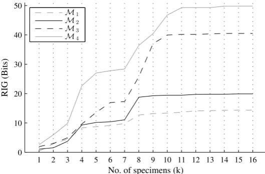
Figure 10 shows the plots of the cumulative sum of values of RIG from a sequence of

specimen fatigue tests for model classes _M1 to M4. The numbering of the specimen tests

is the actual order in which the experiments were performed. These plots clearly show that

there exist a specific size of the dataset, expressed as a number of test specimens, after which

the inference does not gain significant information. Based on these results, we choose the

value of 11, as the minimum required number of test specimens for adequate inference in

our problem, although this value actually depends on each of model classes. In fact, observe

that the more complex the model is (in the sense of the number of model parameters, as

explained in Section 3.3), the bigger the size of the required dataset, resulting in an optimal

number of specimens from 8 to 11 for model classes_M1 toM4, respectively. Notice also that

more complex models acquire more information from each test. Both of these experimental

observations make sense with the results obtained for the complexity of model classes in the

last section.

4.3. Posterior robust predictive model

As an alternative to selecting a single model class based on the evidence values, a

dam-age model can be obtained based on the complete set of models M through the posterior

hyper-robust predictive PDF of damage [12]. Based on the Total Probability Theorem, this

definition allows us to account for all the probabilistic information in terms of the

uncer-tainty related to both parameters and model class choice for the prediction of damage, as

follows:

p(xn|D,M) = NM X

j=1

p(xn|D,Mj)p(Mj|D,M) (30)

where p(xn|D,Mj) is the posterior robust prediction of damage including the parameter

uncertainty for model class _Mj:

p(xn|D,Mj) = Z

Θ

p(xn|θ,D,Mj)p(θ|D,Mj)dθ (31)

If the posterior probabilities p(_Mj|D,M) given in Table 4 and based on the uniform

priorp(_Mj|M) =1/4(so that all model classes are considered equally plausible a priori) are

substituted into Equation 30, it is clear that the contributions of models_M1 andM4 to the

hyper-robust predictive model in Equation 30 are negligible, and it can be approximated by:

p(xn|D,M)∼= 0.826p(xn|D,M2) + 0.174p(xn|D,M3) (32)

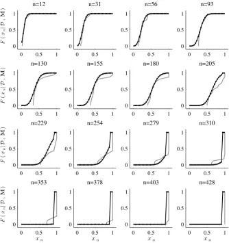
The cumulative distribution function (CDF) F(xn|D,M) based on Equation 32 is plotted

in Figure 11 where it is compared with the empirical CDF based on the data _D, showing

good agreement between these data and the posterior predictions based on models _M2 and

5. Concluding remarks

A new modeling approach based on Markov chains is proposed to deal with the uncertain

physical process and variability of fatigue-based damage in composites. A Bayesian

frame-work is used to quantify and post-process the uncertainty and also to select the optimum

model parameterization for fatigue damage modeling. The overall procedure is demonstrated

using real data for the evolution of damage for glass-fiber composite coupons subject to

tension-tension fatigue.

The following general conclusions are made:

• Accounting for the non-stationarity of the fatigue-damage evolution improves

signifi-cantly the model predictions;

• Based on the posterior information about a set of model classes, a hyper-robust

pre-dictive damage model can be obtained as a multi-model probability density function

that gives a higher level of robustness to modeling uncertainty than just taking the

most probable model in the set of model classes;

• This Bayesian updating framework can also be used in conjunction with a measure of the information gain from a specimen test to select a minimum set of specimens for

damage characterization and prediction, with the ultimate benefit being the avoidance

of unnecessary costs in fatigue experimental programs;

• Other phenomena in composites like matrix-crack density, delamination area, etc., that imply cumulative damage processes, can benefit by applying a similar Bayesian

framework to Markov chain models of the phenomena.

Acknowledgements

The two first authors would like to thank the Education Ministry of Spain for the

grants FPU 2009-4641, FPU 2009-2390 and GGI3000IDIB; and the California Institute

work. The authors would also like to acknowledge the fruitful discussions with Prof. Michael

Ortiz of Caltech and the work of Wei et al. for their valuable set of data published in [20].

The authors also appreciate the reviewers’ efforts on the manuscript to provide valuable

[1] S. Carbillet, F. Richard, E. Boubakar, Reliability indicator for layered composites with strongly

non-linear behaviour, Composites Science and Technology 69 (1) (2009) 81–87.

[2] W. Hwang, K. S. Han, Fatigue of composites-Fatigue modulus concept and life prediction, Journal of

Composite Materials 20 (2) (1986) 154–165.

[3] S. Abrate, Matrix cracking in laminated composites: a review, Composites Engineering 1 (6) (1991)

337–353.

[4] A. S. D. Wang, Strength, failure, and fatigue analysis of laminates, in: Engineered Materials Handbook,

vol. 1, ASM International, 236–251, 1997.

[5] J. Degrieck, W. Van Paepegem, Fatigue damage modeling of fibre-reinforced composite materials:

Review, Applied Mechanics Reviews 54 (4) (2001) 279.

[6] D. An, J.-H. Choi, N. H. Kim, S. Pattabhiraman, Fatigue life prediction based on Bayesian approach

to incorporate field data into probability model, Structural Engineering & Mechanics 37 (4) (2011)

427–442.

[7] X. Guan, R. Jha, Y. Liu, Model selection, updating, and averaging for probabilistic fatigue damage

prognosis, Structural Safety 33 (3) (2011) 242–249.

[8] M. Robinson, M. Crowder, Bayesian methods for a growth-curve degradation model with repeated

measures, Lifetime Data Analysis 6 (4) (2000) 357–374.

[9] R. Cross, A. Makeev, E. Armanios, Simultaneous uncertainty quantification of fracture mechanics based

life prediction model parameters, International Journal of Fatigue 29 (8) (2007) 1510–1515.

[10] Y. Ling, S. Mahadevan, Integration of structural health monitoring and fatigue damage prognosis,

Mechanical Systems and Signal Processing 28 (2012) 89–104.

[11] R. Zhang, S. Mahadevan, Model uncertainty and Bayesian updating in reliability-based inspection,

Structural Safety 22 (2000) 145–160.

[12] J. L. Beck, Bayesian system identification based on probability logic, Structural Control and Health

Monitoring 17 (7) (2010) 825–847.

[13] R. T. Cox, The Algebra of Probable Inference, The Johns Hopkins University Press, 1961.

[14] E. T. Jaynes, Probability Theory: The Logic of Science, (Ed. G.L. Bretthorst), Cambridge University

Press, 2003.

[15] A. Papoulis, Probability, Random Variables, and Stochastic Processes, McGraw Hill, ISBN 0070484481,

1965.

[16] J. L. Bogdanoff, F. Kozin, Probabilistic Models of Cumulative Damage, John Wiley & Sons, ISBN

0-471-88180-5, 1985.

[17] J. D. Rowatt, P. D. Spanos, Markov chain models for life prediction of composite laminates, Structural

[18] R. Ganesan, A data-driven stochastic approach to model and analyze test data on fatigue response,

Computers & Structures 76 (4) (2000) 517–531.

[19] Y. Z. Pappas, P. D. Spanos, V. Kostopoulos, Markov chains for damage accumulation of organic and

ceramic matrix composites, Journal of Engineering Mechanics 127 (9) (2001) 915–926.

[20] B.-S. Wei, S. Johnson, R. Haj-ali, A stochastic fatigue damage method for composite materials based

on Markov chains and infrared thermography, International Journal of Fatigue 32 (2010) 350–360.

[21] S. Johnson, B. Wei, R. Haj-Ali, A stochastic fatigue damage model for composite single lap shear joints

based on Markov chains and thermoelastic stress analysis, Fatigue & Fracture of Engineering Materials

& Structures 33 (12) (2010) 897–910.

[22] Y. Lin, J. Yang, A stochastic theory of fatigue crack propagation, AIAA journal 23 (1) (1985) 117–124.

[23] W.-F. Wu, On the Markov approximation of fatigue crack growth, Probabilistic Engineering Mechanics

1 (4) (1986) 224–233.

[24] K. Sobczyk, B. Spencer, Random Fatigue: From Data to Theory, Academic Press, 1992.

[25] J. A. Bea, M. Doblar´e, L. Gracia, Evaluation of the probability distribution of crack propagation life

in metal fatigue by means of probabilistic finite element method and B-models, Engineering Fracture

Mechanics 63 (6) (1999) 675–711.

[26] W. Wu, C. Ni, Probabilistic models of fatigue crack propagation and their experimental verification,

Probabilistic Engineering Mechanics 19 (3) (2004) 247–257.

[27] M. Giorgio, M. Guida, G. Pulcini, An age- and state-dependent Markov model for degradation

pro-cesses, IIE Transactions 43 (2011) 621–632.

[28] M. Guida, G. Pulcini, A continuous-state Markov model for age- and state-dependent degradation

processes, Structural Safety 33 (6) (2011) 354–366.

[29] K. Sobczyk, Stochastic models for fatigue damage of materials, Advances in Applied Probability 19 (3)

(1987) 652–673.

[30] B. F. Spencer Jr, J. Tang, Markov process model for fatigue crack growth, Journal of Engineering

Mechanics 114 (12) (1988) 2134–2157.

[31] F. Casciati, P. Colombi, L. Faravelli, Fatigue crack size probability distribution via a filter technique,

Fatigue & Fracture of Engineering Materials & Structures 15 (5) (1992) 463–475.

[32] J. Lemaitre, J. Cordebois, J. Dufailly, Sur le couplage endommagement-elasticit, Comptes rendus de

l’Acadmie des Sciences, Paris, B. (1979) 391.

[33] G. Z. Voyiadjis, P. I. Kattan, A comparative study of damage variables in continuum damage mechanics,

International Journal of Damage Mechanics 18 (4) (2009) 315–340.

[34] F. N. Fritsch, R. E. Carlson, Monotone piecewise cubic interpolation, SIAM Journal on Numerical

[35] R. T. Cox, Probability, frequency and reasonable expectation, American Journal of Physics (17) (1946)

1–13.

[36] E. T. Jaynes, Papers on Probability, Statistics and Statistical Physics, (Ed. R.D. Rosenkrantz), Kluwer

Academic Publishers, 1983.

[37] A. Tarantola, Inverse Problem Theory and Methods for Model Parameters Estimation, SIAM, 2005.

[38] P. Whittle, Some distribution and moment formulae for the Markov chain, Journal of the Royal

Sta-tistical Society. Series B (Methodological) (1955) 235–242.

[39] P. Billingsley, Statistical methods in Markov chains, The Annals of Mathematical Statistics 32 (1)

(1961) 12–40.

[40] F. Liang, C. Liu, J. Chuanhai, Advanced Markov Chain Monte Carlo Methods, Wiley Online Library,

2010.

[41] N. Metropolis, A. W. Rosenbluth, M. N. Rosenbluth, A. H. Teller, E. Teller, Equation of state

calcu-lations by fast computing machines, TheJournal of ChemicalPhysics 21 (1953) 1087–1092.

[42] W. K. Hastings, Monte Carlo sampling methods usingMarkov chains and their applications, Biometrika

57 (1) (1970) 97–109.

[43] A. Gelman, G. Roberts, W. Gilks, Efficient Metropolis jumping rules, Bayesian Statistics 5 (1996)

599–608.

[44] G. Roberts, J. Rosenthal, Optimal scaling for various Metropolis-Hastings algorithms, Statistical

Sci-ence 16 (4) (2001) 351–367.

[45] J. Hoeting, D. Madigan, A. Raftery, C. Volinsky, Bayesian model averaging: A tutorial, Statistical

Science (1999) 382–401.

[46] J. L. Beck, K. V. Yuen, Model selection using response measurements: Bayesian probabilistic approach,

Journal of Engineering Mechanics 130 (2004) 192.

[47] A. E. Raftery, D. Madigan, J. A. Hoeting, Bayesian model averaging for linear regression models,

Journal of the American Statistical Association (1997) 179–191.

[48] S. F. Gull, Developments in maximum-entropy data analysis, Maximum Entropy and Bayesian Methods

(1989) 53–71.

[49] J. L. Beck, L. S. Katafygiotis, Updating models and their uncertainties. I: Bayesian statistical

frame-work, Journal of Engineering Mechanics 124 (4) (1998) 455–462.

[50] L. S. Katafygiotis, H. F. Lam, Tangential projection algorithm for manifold representation in

unidentifi-able model updating problems, Earthquake Engineering & Structural Dynamics 31 (4) (2002) 791–812.

[51] C. Papadimitriou, J. L. Beck, L. S. Katafygiotis, Asymptotic expansions for reliability and moments of

uncertain systems, Journal of Engineering Mechanics 123 (12) (1997) 1219–1229.

stochastic simulation, Journal of Vibration and Control 14 (1-2) (2008) 7–34.

[53] A. E. Gelfand, D. K. Dey, Bayesian model choice: asymptotics and exact calculations, Journal of the

Royal Statistical Society. Series B (Methodological) 56 (3) (1994) 501–514.

[54] S. H. Cheung, J. L. Beck, Calculation of posterior probabilities for Bayesian model class assessment

and averaging from posterior samples based on dynamic system data, Computer-Aided Civil and

In-frastructure Engineering 25 (5) (2010) 304–321.

[55] W. R. Gilks, S. Richardson, D. J. Spiegelhalter, Markov Chain Monte Carlo in Practice, Chapman and

Hall, 1996.

[56] R. Talreja, A continuum mechanics characterization of damage in composite materials, Proc. R. Soc.

London 399 (1985) 195–216.

[57] R. Y. Rubinstein, D. P. Kroese, Simulation and the Monte Carlo Method., John Wiley & Sons, Hoboken,

New Jersey, second edn., 2008.

[58] S. Kullback, R. A. Leibler, On Information and Sufficiency, The Annals of Mathematical Statistics

DAMAGE MODEL

Markov chain PARAMETERIZATIONθ={p, θi, θ_i0, . . .}

DAMAGE PREDICTION

CDF:F(xnk|θ,D); ∀nk∈ TD STOCHASTIC MODELING

BAYESIAN INFERENCE

MODEL CLASS DEFINITION M:{M1 M2 M3. . .MNM} DATA(D)

Krepetitions of fatigue-damage manifestation

POSTERIOR OF PARAMETERS

(Bayes’ Theorem within each model class)

PRIOR PDF FOR MODEL

User’s judgement

MODEL CLASS ASSESSMENT

(Bayes’ Theorem at model classes level) Evidence Computation

ROBUST INFERENCE

(Total Probability Theorem)

p(xn|D,Mj) j: 1, . . . , NM

HYPER-ROBUST INFERENCE

(Total Probability Theorem)

p(xn|D,M)

0 0.2 0.4 0.6 0.8 1 0 0.2 0.4 0.6 0.8 1 θ θ ′

(θ₁,θ′

1)

(θ₂,θ′

2)

∆θ ₌ m−n N

∆θ′_{= g(}m

N)−g(Nn)

θ′_{= g(}θ)

Figure 2: Spline transformation θ0 _{= g(θ) of the unit time scale θ controlled by the set of interpolation}

points_{(0,0),(θ1, θ01), . . .(θj, θ0j),(1,1)}; θj > θj−1 and θ0j > θ0j−1; j >1. The grey line would correspond

to a stationary process in which the time transformation does not take place, soθ0=θ; whereas the darker curve represents the proposed non-stationary scheme.

0 1 2 3 4 5 -6 er er er er

n1 n2 n3 n4 n5 n6 n7 (((( (((       

1 0 1 0 0 0

0 0 0 0 0 0

0 0 0 0 0 0

0 0 0 0 0 0

0 0 0 0 0 0

0 0 0 0 0 0

       Specimen1 Specimen2

Figure 3: Toy example for obtaining fn=n4 when a Markov chain with 6-states is studied with data from

two specimens. The damage states are represented on the vertical axis. The set of DC are represented on the horizontal axis. Observe that a transition between states 1 (forn =n3) and 3 (for n =n4) occurs in

0 100 200 300 400 0

0.1 0.2 0.3 0.4 0.5 0.6 0.7 0.8 0.9 1

n

ˆyn

Figure 4: Experimental sequences of damage for quasi-isotropic notched S2-Glass/E733FR laminates taken from [20].

0.86 0.88 0.9 0.92

0 0.2 0.4

0 0.2 0.4

0.86 0.88 0.9 0.92 0 0.1 0.2 0.3 0.4 0 0.1 0.2 0.3 0.4

θ₁

θ′

1

θ′

1

θ₁

p

p

Figure 5: Plots of 104_{posterior samples in theθ space when updating model classM}

1 with fatigue dataD

0.82 0.84 0.86 0.35 0.4 0.45

0.16 0.2 0.24

0 0.07 0.15

0 0.05 0.1

0.82 0.84 0.86 0.35 0.4 0.45 0.16 0.2 0.24 0 0.07 0.15 0 0.05 0.1

θ₁

θ′

1

θ′

1

θ₂

θ₂

θ′

2

θ′

2

θ₁

p

p

Figure 6: Plots of 104_{posterior samples in theθ space when updating model class}

M2 with fatigue dataD

0.88 0.91 0.53 0.58

0.44 0.56 0.3 0.35

0.18 0.26 0.16 0.22

0.14 0.2 0.88

0.91 0.53 0.58 0.44 0.56 0.3 0.35 0.18 0.26 0.16 0.22 0.14 0.2

θ1

θ′

1

θ′

1

θ2

θ2

θ′

2

θ′

2

θ3

θ3

θ3′

θ′

3

θ1

p

p

Figure 7: Plots of 104_{posterior samples in theθ space when updating model class}

M3 with fatigue dataD

0 0.2 0.4 0.6 0.8 1 0

0.2 0.4 0.6 0.8 1

θ

θ

′

M1

M2

M3

M4

Figure 8: Plots of interpolation curves of unit time transformation for model classes M1 to M4. The

interpolation points are the MAP values of (θi, θ0

i), which are drawn from left to right in increasing order

within their respective curve.

0 50 100 150 200 250 300 350 400 0

0.2 0.4 0.6 0.8 1

n

x

n

Simulated model mean Simulated model std. dev. Data mean (±σ)

(a) B-K model

0 50 100 150 200 250 300 350 400 0

0.2 0.4 0.6 0.8 1

n

x

n

Simulated model mean Simulated model std. dev. Data mean (±σ)

(b)M2

Figure 9: Monte Carlo mean and standard deviation of simulated sequences of damage by using a B-K model (left) and model classM2 (right), in comparison with the mean and standard deviation of

1 2 3 4 5 6 7 8 9 10 11 12 13 14 15 16 0

10 20 30 40 50

No. of specimens (k)

RIG (Bits)

M1

M2

M3

M4

Figure 10: Plots of the cumulative sum of values of the RIG between consecutive posteriorsp(θ_|Dk,_Mj), k= 1, . . . , K, for models classes _M1 toM4. When k= 1, the RIG aboutθ is computed fromD1 relative

0 0.5 1 0 0.5 1 n=12 F ( xn |D , M )

0 0.5 1

0 0.5 1

n=31

0 0.5 1

0 0.5 1

n=56

0 0.5 1

0 0.5 1

n=93

0 0.5 1

0 0.5 1 n=130 F ( xn |D , M )

0 0.5 1

0 0.5 1

n=155

0 0.5 1

0 0.5 1

n=180

0 0.5 1

0 0.5 1

n=205

0 0.5 1

0 0.5 1 n=229 F ( xn |D , M )

0 0.5 1

0 0.5 1

n=254

0 0.5 1

0 0.5 1

n=279

0 0.5 1

0 0.5 1

n=310

0 0.5 1

0 0.5 1 n=353 F ( xn |D , M ) xn

0 0.5 1

0 0.5 1

n=378

xn

0 0.5 1

0 0.5 1

n=403

xn

0 0.5 1

0 0.5 1

n=428

xn

Model Class Parameters

M1 θ1 θ

0

1 - - - p

M2 θ1 θ

0

1 θ2 θ 0

2 - - - p

..

. . ..

MNM θ1 θ

0

1 θ2 θ 0

2 . . . θNM θ

0

NM p

Table 1: Parameterization scheme for the setM ofNmmodel classes

M1 M2 M3 M4

σq 0.007 0.005 0.005 0.0035

N1 104 104 104 104

Burn-in 400 400 500 700

Acc-rate 23% 34% 37% 40%

Table 2: Metropolis-Hastings algorithm configuration together with results of the acceptance rate for the stochastic simulation used for inferring models_M1 toM4.

θ1 θ

0

1 θ2 θ

0

2 θ3 θ

0

3 θ4 θ

0

4 p

MAP 0.1083 0.1080 – – – – – – 0.89

M1 c.o.v. (%) 45.31 48.76 – – – – – – 0.75

std 0.0514 0.0569 – – – – – – 0.0068

MAP 0.0593 0.0618 0.2042 0.4207 – – – – 0.8516

M2 c.o.v. (%) 28.67 31.54 09.84 05.27 – – – – 0.13

std 0.0167 0.0213 0.0194 0.0223 – – – – 0.0110

MAP 0.1573 0.1898 0.2051 0.3212 0.4587 0.5454 – – 0.89

M3 c.o.v. (%) 13.64 13.73 09.65 04.91 09.36 03.22 – – 0.97

std 0.0219 0.0264 0.0202 0.0161 0.0428 0.0174 – – 0.0087

MAP 0.1254 0.1719 0.1652 0.3715 0.4131 0.5941 0.7137 0.9353 0.8762

M4 c.o.v. (%) 30.06 33.05 10.62 05.07 07.27 05.80 10.40 01.61 02.09

std 0.0312 0.0449 0.0188 0.0173 0.0308 0.0348 0.0721 0.0152 0.0180

Log evidence Datafit EIG Posterior Probability

M1 -183.43 -180.31 3.11 3.5·10−18

M2 -166.13 -161.61 4.52 0.826

M3 -166.73 -157.05 9.68 0.174

M4 -170.73 -156.25 14.47 1.74·10−5