index selection rules for pivot algorithms of linear programming.
European Journal of Operational Research, 211 (3). 491–500. ISSN
0377-2217 , http://dx.doi.org/10.1016/j.ejor.2012.02.008
This version is available at
https://strathprints.strath.ac.uk/28229/
Strathprints is designed to allow users to access the research output of the University of Strathclyde. Unless otherwise explicitly stated on the manuscript, Copyright © and Moral Rights for the papers on this site are retained by the individual authors and/or other copyright owners. Please check the manuscript for details of any other licences that may have been applied. You may not engage in further distribution of the material for any profitmaking activities or any commercial gain. You may freely distribute both the url (https://strathprints.strath.ac.uk/) and the content of this paper for research or private study, educational, or not-for-profit purposes without prior permission or charge.
Any correspondence concerning this service should be sent to the Strathprints administrator: [email protected]
The Strathprints institutional repository (https://strathprints.strath.ac.uk) is a digital archive of University of Strathclyde research outputs. It has been developed to disseminate open access research outputs, expose data about those outputs, and enable the
Report 2010-02
The s-Monotone Index Selection Rules
for Pivot Algorithms of Linear
Programming
Zsolt Csizmadia and Tibor Ill´
es
May 2010
E¨
otv¨
os Lor´
and University of Sciences,
Budapest, Hungary
http://www.cs.elte.hu/opres/orr/
The s-Monotone Index Selection Rules
for Pivot Algorithms of Linear
Programming
Zsolt Csizmadia and Tibor Ill´
es
Abstract
In this paper we introduce the concept ofs-monotone index selection rule for linear programming problems. We show that several known anticycling pivot rules like the minimal index-, last-in-first-out- and the-most-often-selected-variable pivot rules ares-monotone index selection rules. Furthermore, we show a possible way to define news-monotone pivot rules. We prove that several known algorithms like the primal (dual) simplex- and MBU-simplex algorithms and criss-cross algorithm withs-monotone pivot rules are finite methods. Therefore, one possible research direction in the area of pivot algorithms might be to find s -monotone index selection rules that have interesting properties either from theoretical or from computational (for example larger flexibility in pivot selection) viewpoint.
Keywords: linear programming problem, pivot algorithms, anti-cycling pivot rules, s-monotone index selection rules.
2000 Mathematics Subject Classification: 49M35,90C20.
1
Introduction
LetA∈IRm×n
,c∈IRn
,b∈IRmbe matrix and vectors respectively, then
is aprimal linear programming (P-LP) problem. While the dual linear pro-gramming (D-LP) problemcan be defined as follows
maxbTy ATy≤c
wherex∈IRn andy∈IRmare primal- and dual decision vectors, respec-tively.
Linear programming problems might be solved by applying pivot algo-rithms. The finiteness of the pivot algorithms depend on the algorithms property itself (pivot selection rule, anti-cycling strategy etc.).
Pivot based methods (like the simplex algorithm [6], MBU simplex algo-rithm [1] or the criss-cross algoalgo-rithm [15, 11, 12]) often features the following similar principles:
1. The main flow of the algorithm is defined by a pivot selection rule
which defines the basic characteristics of the algorithm, tough the pivot position defined by it is not necessary unique (see for instance [6, 10, 4]), a series of ”wrong” choices may even lead to cycling [10, 4].
2. To avoid the possibility of cycling, an index selection rule is used as an anti-cycling strategy (see for instance [3, 4, 13]), which may be flexible [5, 7] but usually at several basis during the algorithm, it defines the pivot position uniquely.
For several pivot algorithms – like simplex-, MBU simplex or criss-cross algorithms –, proofs of finiteness are often based on the orthogonality theorem [9, 2], considering a minimal cycling example [2], and following the movements of the least preferred variable of the index selection rule [3, 14, 7, 8]. Examples of such rules include
1. Pivot selection rules for (P-LP):
(a) Simplex[6] (Pivot column selection: negative reduced cost. Pivot element selection: using ratio test. Preserving non negativity of the right hand side.)
(c) Criss-cross [12] (Pivot column/row selection is based on infeasi-bility – negative right hand side or negative reduced cost. Pivot element selection: admissible pivot positions.)
2. Index selection rules:
(a) Bland’s minimal index rule (b) last-in-first-out (LIFO)
(c) most-often-selected-variable (MOSV)
LIFO and MOSV rules for linear programming problems were first used by S. Zhang [14] to prove the finiteness of the criss-cross algorithm with these anti-cycling index selection rules. Bilen, Csizmadia and Illˇd˙z˝s [2] proved that variants of MBU simplex algorithm are finite with both LIFO and MOSV index selection rules, while Csizmadia in his PhD Thesis [5] showed that the simplex algorithm is finite when the LIFO and MOSV are applied. These results led to the joint generalization of the above mentioned anti-cycling index selection rules.
Without loss of generality we may assume that therank(A) =m. Let us associate to (P-LP) the (primal) pivot tableau
A b
cT *
and let us assume thatAB is an m×m regular submatrix of the matrixA,
thus form a basis of the linear systemAx=b. In this case the (primal) basic pivot tableau associated with the (P-LP) problem and basisAB is
A−B1A A−B1b
cT −cT BA
−1
B A −cBA −1
B b
The variables corresponding to the column vectors of the basisAB are called
basic variables. The index set of basic and nonbasic variables will be denoted by IB and IN, respectively. Let us introduce the following notations T =
A−B1A, b¯ =AB−1b, ¯c=c−cBA −1
B A. Now we are ready to define (column)
vectorst(i)andt
tableau of the (P-LP) problem, wherei∈ IB andj∈ IN, respectively, in the
following way:
(t(i))k=tik=
tik if k∈ IB∪ IN
¯
bi if k=b
0 if k=c
and
(tj)k =tkj=
tkj if k∈ IB
−1 if k=j
0 if k∈(IN \ {j})∪ {b}
¯
cj if k=c
where b andc denotes indices associated with vectors bandc, respectively. Furthermore, we definet(c) andt
b vectors in the following way
(t(c))k=tck=
¯
ck if k∈ IB∪ IN
1 if k=c −cT
BA −1
B b if k=b
and
(tb)k=tkb=
¯bk if k∈ IB
−1 if k=b
0 if k∈ IN
−cT BA
−1
B b if k=c
and from now on we assume thatcis always a basic index, whilebis always a nonbasic index of the (P-LP) problem. Now we are ready to state the version of the orthogonality theorem that we frequently use in the finiteness proof of pivot algorithms that have anti-cycling index selection rules.
Result 1.1 (Orthogonality theorem, Klafszky and Terlaky, 1991). Let a (P-LP) problem be given, withrank(A) =mand assume that IB′ and IB′′ are
two arbitrary bases of the problem. Then
(t′′(i))Tt′j= 0 for alli∈ IB′′ and for allj6∈ IB′.
to the new wider class of index selection rules. In section 4 we prove that well-known pivot algorithms like the primal/dual simplex algorithm [6] and the primal/dual monotonic-build-up simplex algorithm [1] withs-monotone index selection rules are finite algorithms for solving linear programming problems. Without proof, we mention that the criss-cross algorithm [12] is also finite withs-monotone index selection rules. Some conclusions and further research questions close our paper.
2
The s-monotone index selection rule
In this section, we introduce a general framework for proving the finiteness of several pivot algorithms and index selection rule combinations mentioned in the previous section.
Definition 2.1 (Possible pivot sequence). A sequence of index pairs
S ={Sk= (ik, ok) :ik, ok ∈IN for some consequitive k∈IN},
is called apossible pivot sequence, if (i) n= max{max
k∈IN
ik,max k∈IN
ok}is finite,
(ii) there exists a(P-LP) withnvariables and therank(A) =m, and (iii) (possibly infinite) pivot sequence, where the moving variable pairs of
(P−LP) correspond to the index pairs ofS.
The index pairs of a possible pivot sequence thus only required to comply with the basic and nonbasic status. It is now easy to show that
Proposition 2.1. If a possible pivot sequence is not finite then there exists a (sub)set of indices,I∗
, that occur infinitely many times inS.
Let us introduce the concept ofpivot index preference.
Definition 2.2 (Pivot index preference). A sequence of vectors sk ∈ Nn is
called a pivot index preference of an index selection rule, if in iteration j, in case of ambiguity according to a pivot selection rule, the index selection rule selects an index with highest value insj among the candidates.
Definition 2.3 (s-monotone index selection rules). Letn∈IN be given. An index selection rule is calleds-monotone, if
1. there exists a pivot index preferencesk ∈Nn, for which
(a) the values in the vectorsj−1after iterationj may only change for
ij and oj, where ij and oj are the indices involved in the pivot
operation,
(b) the values may not decrease.
2. For any infinite possible pivot sequenceS and for any iterationj there exists iterationr≥j such that
(a) the index with minimal value in sr among I∗∩ IBr is unique (let
it bel), whereIBr is the set of basic indices in iterationr, andI
∗
is the set of all indices that appear infinitely many times inS, (b) in iterationt > rwhen index l∈ I∗
occurs again inS for the first time, the indices ofI∗ that occurred inS strictly between
Srand
Sthave a value insthigher than the indexl.
3
s-monotone index selection rules
In this section we prove the following
Theorem 3.1. The
1. minimal index rule,
2. the most-often-selected variable rule and
3. the last-in first-out index selection rule
ares-monotone index selection rules.
The proof of this theorem follows from the following observation and two lemmas.
For the minimal index rule let us set each vector sk to be equal to the
vector (n, n−1, . . . ,1)T. Then it is easy to show that the minimal index rule
Lemma 3.2. The LIFO index selection rule is s-monotone index selection rule.
Proof. Let us initiate the vector s to be the zero vector. In a pivot when
xik leaves and xok enters the basis in the k
th iteration, the values of s are
modified to favor these variables:
s′ i=
k ifi∈ {ik, ok},
si otherwise,
and assume that a possible pivot sequenceSis generated using the pivot index preference.
It is clear that the series ofs vectors defined in such a way, form a pivot index preference for the LIFO rule. Furthermore, it is obvious that the prop-erties 1 (a) and 1 (b) of thes-monotone index selection rule are satisfied.
In case of an infinite possible pivot sequence and an arbitrary iteration j
either all thesi, i∈ I∗∩ IBj values are already different or if some have the
same (initial) value, meaning they have not moved yet, then there should be an iteration later when these variables move for the first time. Let us denote that iteration byrwhen the last variable having index fromI∗
moves for the first time. Then for the vectorsr2 (a) holds. Property 2 (b) follows from the
definition of update for vectors.
Now, we are ready to prove that the most-often-selected variable rule is an
s-monotone index selection rule, too.
Lemma 3.3. The MOSV index selection rule is s-monotone index selection rule.
Proof. Let the vector sbe initialized as the zero vector. In a pivot when
xik leaves and xok enters the basis in the k
th iteration, the values of s are
modified to increase the favor of these variables:
s′i=
si+ 1 ifi∈ {ik, ok},
si otherwise,
and assume that a possible pivot sequence S is generated using the pivot index preference that defines the pivot index preference for MOSV. Due to the definition of the MOSV update, the properties 1 (a) and 1 (b) of the
s-monotone index selection rule is satisfied.
For any infinite possible pivot sequence, define I∗
set of nonbasic indices for the jth iteration and let M
N = INj ∩ I
∗
and
MB=I∗\ MN. We define the numbersγi as follows:
γi=
si, ifi∈ MN
si+ 1, ifi∈ MB
Let
P ={i∈ I∗
|i∈arg min
k∈I∗ γk} and kmin∈I∗ γk =ρ.
We continue to update s according to the possible pivot sequence. Since
P ⊂ I∗
, thus for any i∈ P there exists such an iteration, when variable xi
enters the basis for the first time after iteration j. When this happens, we delete its index fromP, thusP :=P \{i}. After finitely many iterations, such a setPis obtained, for which| P |=| {l} |= 1. After this happens, let the first iteration when variablexlenters ber. We show that in iterationrthe choice
ofxl is unique. Observe, that in this casesl =ρ, regardless whetherxl was
moving in iterationj or not. Because of the pivot rule, ρ < si if i∈ I∗\ P
and since every variable with indexi∈ P \ {l} has at least once entered the basis after iterationj and now is outside the basis, their values insmust be at leastρ+ 2. On the other hand, if it was a basic variable in iterationjthen itssvalue is at leastρ+ 1. Thus 2 (a) also holds.
Since the variablexlenters the basis in iterationr, and every other variable
with index inI∗entering the basis after
xlalready had a highersvalue than
xl in basisIBr, according to the MOSV rule, thus 2 (b) also holds.
Analyzing the proofs of the previous two lemmas we can conclude that the 1 (a) and 1 (b) requirements of the definition ofs-monotone index selection rule are satisfied with the proper update strategy used to define the pivot index preference. Proving property 2 (a) there are three important ingredients: (i) the assumption that the pivot sequence is infinite, (ii) the finiteness of the index set, and (iii) the monotone increasing property of the pivot index preference, namely that for the vectors sk+1,sk ∈ IRn : sk+1 ≥ sk and
sk+16=sk hold for any iterationk∈IN. Property 2 (b) explains the changes
in the s-values of those variables that belong to the index set I∗ and have
moved between two consecutive moves of the least preferred variable. This property depends strongly on the monotonicity of the pivot index preference and on the property 2 (a), too.
Let the vectorsbe initialized as the zero vector. In a pivot whenxik leaves
and xok enters the basis in the k
th iteration, the values ofsare modified to
increase the favor of these variables.
Generalized-last-in-first-out rule (GLIFO): Let us consider astrictly mono-tone increasingsequence of positive rational numbers, namely for all k∈IN indicespk+1> pk hold.
s′i=
pk ifi∈ {ik, ok},
si otherwise,
It is quite easy to show that this slight modification of the pivot index preference of LIFO rule will lead to an s-monotone index selection rule, too. Namely, all the steps of the proof of Lemma 3.2, remains true; in fact after each variable that moves at all has moved at least once the sequences defined by GLIFO are the same as those by LIFO.
However, the generalization of MOSV define a significantly more general class of pivot sequences. We can generalize the MOSV rule as well by modi-fying its pivot index preference.
Generalized-most-often-selected-variable rule (GMOSV): Let us consider a monotone increasing sequence of positive rational numbers, namely for all
k∈IN indicespk+1≥pk hold.
s′i=
si+pk ifi∈ {ik, ok},
si otherwise,
However, to show that GMOSV is ans-monotone index selection rule we need a slightly more careful analysis of the proof of Lemma 3.3.
The requirements 1 (a) and 1 (b) are simply satisfied because of the defi-nition of the corresponding pivot index preference. Justifying 2 (a), we need to modify the definition ofγi introduced in the proof of Lemma 3.3, slightly.
Let
γi=
si, ifi∈ MN
si+pj, ifi∈ MB
since we would like to analyze the situation in the iteration j. Taking into consideration the monotone increasing nature of thepk sequence we are able
to identify - after finitely many iterations - the least preferred variable xl in
some iterationr.
Showing the uniqueness of the choice of xl in the iteration r we need to
sl=ρ, regardless whetherxlwas moving in iteration j or not. Furthermore,
because of the monotone increasing nature of the pk sequence, ρ < si if
i∈ I∗\ P and since every variable with index
i∈ P \ {l} has at least once entered the basis after iteration j and now is outside the basis, their values ins must be at leastρ+pu+pv, wherer > u, v > j. On the other hand, if
it was a basic variable in iterationj than itssvalue is at leastρ+pu, where
r > u > j. Since pu ≥pj and pv ≥pj hold we have verified that 2 (a) also
holds.
Our last task is to show that 2 (b) holds as well. For this, let us collect all available information, namely we know that at the iteration r the following inequalities
sr
l < sri, ∀i∈ I ∗
\ {l}
hold and thatst l =s
r
l +pr. Leti∈ I∗\ {l} be the index of such variablexi
that has moved between the iterationr and t, at least once, for instance in iterationk, wheret > k > r holds. Then
sti≥s k+1
i =s
k
i +pk ≥ski +pr≥sir+pr> srl +pr=stl,
thus 2 (b) is really satisfied.
Now we are ready to state our following result
Lemma 3.4. GLIFO and GMOSV index selection rules ares-monotone index selection rule.
It is easy to check that when the sequence whenpk = 1, for all k, then
GMOSV become MOSV, and that GMOSV is indeed a generalization of MOSV (e.g. it allows for switching from MOSV to LIFO).
4
Finiteness of pivot algorithms with
s-monotone index selection rules
In this section we show that simplex-, MBU simplex- and criss-cross algo-rithms with s-monotone index selection rules are finite for linear program-ming problem. The proofs are based on the same ingredients: (i) assume contrary that the algorithm is cycling, namely that there are variables that enters/leaves bases infinitely many times, (ii) choose a minimal cycling ex-ample and denote the indices of those variables that moves infinitely many times byI∗
iterations when the least preferred variable enters/leaves bases, (v) during a cycle corresponding pairs of almost terminal tableaus should occur to com-plete the cycle, however this contradicts to the orthogonality theorem. Thus, in this framework, the only important step is to properly identify the almost terminal tableaus and to read out from the row/column the sign structure which will show the contradiction based on the orthogonality theorem. The structure of the almost terminal tableaus for different pivot algorithms might be slightly different.
4.1
The primal simplex algorithm with s-monotone
index selection rules
The primal simplex algorithm with s-monotone index selection rules
Input: A∈Rm×n,b∈Rm,c∈Rn a feasible basisB, initializedsvector.
Output: An optimal solution, or a certificate that the solution is unbounded.
Begin
I−
N:={i∈ IN|¯ci<0}.
While I−
N6=∅ do
Letq∈ {i∈ I−
N|¯ci<0}be arbitrary with maximal value respect tos. If tq≤0 then
Stop: problem is unbounded, certificate istq. Else
Letϑ:= minn¯bi
tiq |i∈ IB, tiq>0
o
be the value of the primal ratio test.
Letp∈ IB arbitrary, such that ¯ bp
tpq =ϑand with maximal value respect tos.
Endif
Pivot on (p, q).
Endwhile
The solution is optimal.
End.
It is easy to verify that in a minimal cycling example all the variables are moving during a cycle and that the right hand side values are zeros (any nondegenerate pivot would improve the objective). Thus the minimal cycling example should be completely primal degenerate.
xl
+ 0
0
.. .
0 0
.. .
0
− ⊕ . . . ⊕
xk
xl + 0
K + .. . + 0 .. . 0 L ⊖ .. . ⊖ 0 .. . 0 −
xlleaves the basis B′′
Consider basisB′
of the minimal cycling example, when the least preferred variable xl enters the basis. According to the column selection rule of the
simplex algorithm, the objective function row of the pivot tableau for basis
B′
has a negative entry for the nonbasic variablexl and nonnegative entries
for all other nonbasic variables. (This is the structure of our first almost terminal pivot tableau.)
In a minimal cycling example, since every variable moves infinitely many times, variablexlmust leave the basis. Consider basisB′′ whenxlleaves the
basis for the first time afterB′. According to the s-monotone index selection
rule, the choice of the leaving variable is selected from those basic variables that are least preferred, in our case xl is a such variable. (This defines our
second almost terminal pivot tableau.)
Consider the vector t′(c) corresponding to the objective function row for
basisB′ and the vectort′′
k corresponding to the entering variablexk for basis
B′′. Let
K={i∈ IB′′ |t′′ik>0} \ {l}, and L={j∈ IB′′|t′′jk≤0}.
Then
t(c)′Tt′′k =X
i∈K t′ cit ′′ ik+ X j∈L t′ cjt ′′ jk+t
′ clt
′′ lk≤t
′ clt
′′ lk,
using thatt′
cj≥0 andt ′′
jk≤0 for allj ∈ L, andt ′
ci= 0 for alli∈ Kbecause of
the 1 (b) criterion, the values ofsmay not decrease, and those variables that have moved since basisB′
have a greater value insthan variablexl. By the 2
(b) criterion ofs-monotone index selection rule, the variables corresponding to the index setK, have not moved since basisB′
value int′(c). Since t′
cl <0 andt ′′
lk >0, we have t
(c)′T
t′′
k <0, contradicting
the orthogonality theorem. This proves that the primal simplex algorithm withs-monotone index selection rules are finite.
4.2
The primal MBU simplex algorithm with s-monotone
index selection rules
The primal MBU simplex algorithm with s-monotone index selection rules
Input: A∈Rm×n,b∈Rm,c∈Rn a feasible basisB.
Output: An optimal solution, or a certificate that the solution is unbounded.
Begin
Initialize vectors. IN−:={i∈ IN|¯ci<0}. WhileI−
N6=∅do
Let the driving variables∈ {i∈ IN|¯ci<0}be arbitrary. While ¯cs<0do
LetKs={i∈ IB|tis>0}.
If Ks=∅ thenStop: problem is unbounded, certificate ists. Else
Letϑ:= minn¯bi
tis|i∈ Ks
o
the value of the primal ratio test.
Letr∈ Ks arbitrary such that t¯br
rs =ϑand with maximal value respect tos.
Letθ1:=|tc¯rss|, and letJ ={i∈ IN|¯ci≥0, tri<0}.
If J =∅then
θ2:=∞. Else
θ2:= min n
¯ ci
|tri||i∈ J
o
the value of the dual ratio test. Letq∈ J arbitrary such thatθ2= ¯
cq
|trs| and with maximal value respect tos.
Endif
If θ1≤θ2 then
Pivot on (r, s), (driving pivot).
Else
Pivot on (r, q), (auxiliary pivot).
Endif Endif Endwhile Endwhile
The solution is optimal.
End
To establish the correctness of the algorithm, we repeat the key theorems proved in [1]. We will call a pivot in the column of the driving variable a
driving pivot, while any other pivot an auxiliary pivot.
Result 4.1 (Anstreicher and Terlaky, 1994). Consider any pivot sequence produced by the primal MBU simplex algorithm corresponding to an initial feasible basis and the choice of a driving variable xs. Then following an
auxiliary pivot, the next basis produced by the algorithm has the following properties:
1. ¯cs<0,
2. if ¯bi<0, thentis<0,
3. maxn¯bi
tis |
¯bi<0o
≤minn¯bi
tis |tis>0
o
.
It may happen that auxiliary pivot destroys primal feasibility. Next result of Anstreicher and Terlaky [1] states that the primal feasibility is restored after a driving pivot.
Result 4.2 (Anstreicher and Terlaky, 1994). Whenever the primal MBU simplex algorithm performs a driving pivot, the next basis is primal feasible. Based on the previous theorems, we may state that the MBU algorithm is well-defined, [1].
Note that if the problem is both primal and dual nondegenerate, then finiteness is ensured by the fact that similarly to the simplex method, the objective function strictly increases in each iteration [1].
In the original paper [1], lexicography was used to ensure finiteness for degenerate problems. In this section, we prove that the algorithm is finite whenevers-monotone pivot rules are applied. First, we need to examine some further properties of the algorithm.
Lemma 4.1. Both driving- and auxiliary pivots may only increase the reduced cost of the driving variable.
Proof. A driving pivot makes the dual infeasible driving variable dual feasi-ble, while an auxiliary pivot increases the reduced cost of the driving variable without making it nonnegative, or leaves it unchanged. (Follows from the Theorem 4.1.)
The next lemma states a further monotone property of the primal MBU simplex algorithm.
Lemma 4.2. In any sequence of auxiliary pivots generated by the algorithm for driving variablexr, the value max
n¯
bi
tis |
¯
bi<0
o
Proof. Note that the third condition of Theorem 4.1 holds for any sequence of auxiliary pivots (see proof in [1]), thus
max
¯
bi
tis
|¯bi<0
≤min
¯
bi
tis
|tis>0
(1)
always holds. Observe, that by the primal ratio test carried out by the al-gorithm, for an auxiliary pivot made on position (r, q), the minimal ratio of minn¯bi
tis |tis>0
o
is obtained, i.e. ¯ br trq = min ¯ bi tis
|tis>0
.
If we denote the tableau after the pivot ontrq by ˆT and the new right hand
side by ˆb, then
ˆ
trq =
trq
trq
= 1, bˆr=
¯
br
trq
<0, ˆbr
ˆ
trq
= ¯br
trq
since trq < 0 and ¯br > 0, thus since the auxiliary pivot is carried out on a
negative pivot element, the new right-hand side value for index r becomes negative, while the ratio of the right-hand side and the pivot element remain the same. This means in the next iteration this ratio occurs in the left-hand side of (1).
Before examining a possible cycling example, we need a technical-type lemma. This lemma plays a fundamental role in the proof of finiteness with
s-monotone pivot rules.
Lemma 4.3. Let a, b,Θ∈Rsuch thatb6= 0 and a
b = Θ. Letc, d, λ∈Rsuch
that d·λ6= 0 andb+λd6= 0. Then if a+λc
b+λd = Θ, then c d = Θ.
Proof.
a+λc
b+λd = Θ
a+λc = Θ(b+λd) Θ +λc
b = Θ
1 +λd b
c
b = Θ
d b c
We are ready to prove that the MBU simplex algorithm withs-monotone pivot rules is finite. Our proof is based on contradiction. Let us consider a minimal example, for which the algorithm is not finite. As usual, since the number of possible bases is finite, the algorithm must visit the same basis in-finitely many times. It is clear, that because of minimality, in such an example each variable moves infinitely many times, with the possible exception of one single variable, which may remain an infeasible driving variable throughout the whole cycle.
Lemma 4.4. Let us assume that we would like to solve a minimal cycling example using primal MBU simplex algorithm. The following properties hold:
1. Any basis generated by the algorithm is dual degenerate for all variables except one single variable. This variable remains the same throughout the algorithm and never enters the basis.
2. All variable moves infinitely many times, except one, which never enters the basis.
3. No driving pivot is made.
4. The primal ratio test always yields the same value. Furthermore, in any basis generated by the algorithm, for the column r of the driving variable, the ratio ¯bi
tir is the same for alli, wheretir6= 0.
Proof. By Lemma 4.1, a pivot made in a nondegenerate column strictly increases the value of the driving variable. Observe, that while a pivot in a nondegenerate column leaves the column of the short pivot tableau nonde-generate, a degenerate pivot doesn’t change the row of the objective function in the tableau.
It is easy to see, that in a cycling example, there exists an infeasible driving variable xr that never becomes feasible, thus once this variable is selected
for the role of a driving variable, only auxiliary pivots are made. Because the problem is a minimal cycling example, all other variables should move infinitely many times. However, by the observation made above, namely that ¯
ci= 0 for alli6=r, so it follows that 1 holds.
Statements 2 and 3 follow immediately from 1.
By Lemma 4.4, a minimal cycling example contains a single infeasible dual variable selected as driving variable. Furthermore, both the primal and dual ratio tests are trivial, and the selection of indices is solely based on the index selection rule. Letxrbe the driving variable. Consider now variablexl with
basis B′ as described in the second criterion ofs-monotone index selection
rules, and let B′′ be the basis when
xl leaves the basis after B′ for the first
time. (Observe, that since the driving variable never enters the basis, l 6=
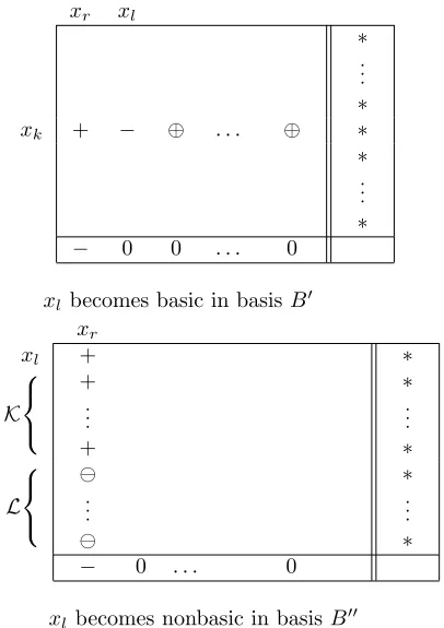
r.) Using the observations stated in Lemma 4.4, the almost terminal pivot tableaux for basesB′ andB′′ have a sign structure as presented in Figure 1.
xr xl
∗
.. .
∗
xk + − ⊕ . . . ⊕ ∗
∗
.. .
∗
− 0 0 . . . 0
xl becomes basic in basisB′
xr
xl + ∗
K
+
.. .
+
∗
.. .
∗
L
⊖
.. .
⊖
∗
.. .
∗
− 0 . . . 0
[image:22.420.114.317.176.464.2]xl becomes nonbasic in basisB′′
Figure 1: Almost terminal pivot tableaux for the MBU simplex algorithm.
We are ready to prove that the algorithm is finite.
rule is finite.
Proof. Let us assume the contrary, and consider a minimal cycling example with entering variable xl and leaving variable xk in basis B′ described in
the second criterion ofs-monotone index selection rules, and basisB′′ when
variablexl leaves the basis for the first time afterB′.
Consider vectort′(k) for basisB′
and vectort′′
r for basisB ′′
. Let
K={i∈ IB′′|t
′′
ir>0} \ {l}, and L={j ∈ IB′′ |t
′′ jr ≤0}.
Then
t(k)′Tt′′r =X
i∈K t′ kit ′′ ir+ X j∈L t′ kjt ′′ jr+t
′ krt
′′ rr+t
′ klt
′′ lr ≤t
′ krt
′′ rr+t
′ klt
′′ lr,
using thatt′
kj≥0 andt ′′
jr ≤0 for allj ∈ L, andt ′
ki= 0 for alli∈ K because
by the first criterion, the values of smay only increase, and those variables that have moved sinceB′
have a greater value insthan variable xl. By the
third criterion of s-monotonicity, these variables have not moved since basis
B′
, thus have a corresponding zero value int′(c). Sincet′
kl <0 and t ′′ lr >0,
furthermoret′
kr >0 and t ′′
rr = −1, we have t(k)
′T
t′′
r <0, contradicting the
orthogonality theorem.
Similar arguments lead to the finiteness proofs of the dual simplex and dual MBU simplex algorithms withs-monotone index selection rule. The finiteness proof of the criss-cross algorithm withs-monotone index selection rule is only slightly different from the previous results. Important details of the finiteness proof for specials-monotone index selection rules can be found in [7, 11, 12]. Thus we can state the following quite general finiteness result of several pivot algorithms.
Theorem 4.6. The primal (dual) simplex- and MBU simplex algorithms and the criss-cross algorithm withs-monotone index selection rules are finite for linear programming problems.
5
Conclusions and further research
Finiteness of the most known pivot algorithms depend on the anti-cycling pivot rules (see [4, 6, 10, 13]). In this paper we have shown that several known index selection rules (minimal index, LIFO, MOSV) possess same monotonicity type property, that has been captured by our new concept, thes-monotone index selection rules. Furthermore, we have introduced new, general anti-cycling pivot rules (GLIFO and GMOSV). We have unified the finiteness proof of some well-known pivot algorithms withs-monotone index selection rules.
Our new concept ofs-monotone index selection rules and the related finite-ness proofs show that anti-cycling pivot rules might leave some freedom of selecting the leaving/entering variable, especially at the initial phase of the computations. However, it is required even from the most flexible anti-cycling pivot rule, to build up an order among the variables at least in such a way that the selection of the least preferred variable become unique at some point of the computation. Form this follows that some strategies of selecting enter-ing variable won’t fulfill this requirement. However, we see some chances to compromise between two different goals: (i) decreasing the objective function in a greedy way, and (ii) guarantee the finiteness of the algorithm.
Suppose that we want to apply thesteepest edgerule for selecting the enter-ing variable and theratio testfor selecting the leaving variable in the (primal) simplex algorithm. Both in the selection of entering or/and leaving variable we might have multiple choices. It is known that the simplex algorithm with the steepest edge rule might cycling, due to primal degeneracy. Our sug-gestion for resolving such situation is the following: keep in mind that you want to have a finite pivot algorithm and apply the steepest edge rule if you have multiple choices for entering variables. Let us formalize a GLIFO and GMOSV index selection rule based on these ideas.
GLIFO with steepest edge index selection rule. Let us assume that
s0=0. In thekth iteration let
Ck−1={i∈ IN : ¯ci<0}, ρ= min
i∈Ck−1sk−1,i and Sk−1={i∈ Ck−1:ρ=sk−1,i}.
If | Sk−1 |= 1 then we have no choice, the index of the entering variable is
steepest edge index selection rule applied onSk−1only. Let
γ=− min
i∈Sk−1
¯
ci
ktik
,
then we can define
pk=
pk+δ ifpk−1≥γ,
γ ifpk−1< γ,
whereδ >0 is a given number. The sequencepk satisfies the strictly
mono-tonic increasing property, therefore we can use it to define, the new values of
sk as follows
sk,i=
pk ifi∈ {ik, ok},
si otherwise.
Similarly we can define GMOSV with steepest edge index selection rule. The main difference is that in the definition of the sequencepk, the number
δmight be zero as well. Furthermore, the rule for updating the sk values is
exactly the same as in the general case for GMOSV.
In many implementations of the simplex algorithm, small random pertur-bations are used instead of index selection methods to ensure finiteness of the algorithm. One possible practical application of the ideas in this paper might be the simplex algorithms with arbitrary precision real number representa-tions, where perturbation is impractical.
Acknowledgements. This research has been supported by the Hungar-ian National Research Fund OTKA No. T 049789. Research of Tibor Ill´es has been partially supported by the project ”Simulation and optimization: basic research in numerical mathematics”sponsored by the frame TAMOP 4.2.2, Hungarian National Office of Research and Technology with the finan-cial support of the European Union from the European Sofinan-cial Fund.
Tibor Ill´es acknowledges the research support obtained from Strathclyde University, Glasgow under theJohn Anderson Research Leadership Program.
References
[2] F. Bilen, Zs. Csizmadia, and T. Ill´es. Anstreicher-terlaky type monotonic simplex algorithms for linear feasibility problems. Optimization Methods and Softwares, 22(4):679–695, 2007.
[3] R.G. Bland. New finite pivoting rules for the simplex method. Mathemat-ics of Operations Research2:103-107, 1977.
[4] V. Chv´atal. Linear Programming. W. H. Freeman an Company, New York, 1983.
[5] Zs. Csizmadia. New pivot based methods in linear optimization, and an application in petroleum industry. PhD Thesis, E¨otv¨os Lor´and University of Sciences, Budapest, Hungary, 2007. www.cs.elte.hu/∼csisza
[6] G.B. Dantzig. Linear Programming and Extensions. Princeton University Press, Princenton, New Jersey, 1963.
[7] T. Ill´es and K. M´esz´aros. A new and constructive proof of two basic results of linear programming. Yugoslav Journal of Operations Research
11(1):15-30, 2001.
[8] T. Ill´es and T. Terlaky. Pivot versus interior point methods: pros and cons. European Journal of Operational Research, 140(2):170-190, 2002. [9] E. Klafszky and T. Terlaky. The role of pivoting in proving some
funda-mental theorems of linear algebra. Linear Algebra and its Applications, 151:97–118, 1991.
[10] K.G. Murty. Linear and Combinatorial Programming. John Wiley & Sons, Inc., New York, 1976.
[11] T. Terlaky. A finite “criss-cross method” for solving linear programming problems [in Hungarian]. Alkalmazott Matematikai Lapok, 10(3-4):289– 296, 1984.
[12] T. Terlaky. A convergent criss-cross method. Optimization, 16(5):683– 690, 1985.
[13] T. Terlaky and S. Zhang. Pivot rules for linear programming: a survey on recent theoretical developments. Annals of Operations Research, 46/47(1-4):203–233, 1993.
2003-01 Zsolt Csizmadia and Tibor Ill´es, New criss-cross type algo-rithms for linear complementarity problems with sufficient matrices.
2003-02 Tibor Ill´es and ´Ad´am B. Nagy, A sufficient optimality criteria for linearly constrained, separable concave minimization problems.
2004-01 Tibor Ill´es and Marianna Nagy, The Mizuno–Todd–Ye predictor– corrector algorithm for sufficient matrix linear complementarity prob-lem.
2005-03 Bilen Filiz, Zsolt Csizmadia and Tibor Ill´es , Anstreicher-Terlaky type monotonic simplex algorithms for linear feasibility prob-lems.
2005-04 Tibor Ill´es, M´arton Makai, Zsuzsanna Vaik, Railway En-gine Assignment Models Based on Combinatorial and Integer Program-ming.
2007-02 Tibor Ill´es, Marianna Nagy and Tam´as Terlaky, An EP theorem for dual linear complementarity problem.