On the modelling of isothermal gas flows at the microscale

On the modelling of isothermal gas flows at the micro scale

DUNCAN A. LOCKERBY1AND JASON M. REESE2

1 _{School of Engineering, University of Warwick, UK ([email protected])} 2 _{Department of Mechanical Engineering, University of Strathclyde, UK ([email protected])}

This paper makes two new propositions regarding the modelling of rarefied (non-equilibrium), isothermal gas flows at the micro scale. The first is a new test case for benchmarking high-order, or extended, hydrodynamic models for these flows. This standing, time-varying shear wave problem does not require boundary conditions to be specified at a solid surface, so is useful for assessing whether fluid models can capture rarefaction effects in the bulk flow. We assess a number of different proposed extended hydrodynamic models, and we find the R13 equations perform the best in this case.

Our second proposition is a simple technique for introducing non-equilibrium effects caused by the presence of solid surfaces into the computational fluid dynamics framework. By combining a new model for slip boundary conditions with a near-wall scaling of the Navier-Stokes constitutive relations, we obtain a model that is much more accurate at higher Knudsen numbers than the conventional second-order slip model. We show this provides good results for combined Couette/Poiseuille flow, and that the model can predict the stress/strain-rate inversion that is evident from molecular simulations. The model’s generality to non-planar geometries is demonstrated by examining low-speed flow around a micro-sphere. It shows a marked improvement over conventional predictions of the drag on the sphere, although there are some questions regarding its stability at the highest Knudsen numbers.

1. Introduction

A number of competing high-order equation sets have been developed in recent years in order to model rarefied gas flows within an efficient continuum-fluid framework (see Reese et al. 2003; Struchtrup 2005). These methods have shown promise, to varying degrees, in predicting certain non-equilibrium behaviour in high-speed as well as micro-scale gas flows at a fraction of the computational cost of molecular-based simulations. However, good predictions of, for example, the viscous structure of one-dimensional shock waves have not always been matched by similarly compelling success in modelling micro-scale gas flows. The primary difficulty is that, unlike the shock wave case, micro gas flows tend to be dominated by the influence of solid bounding surfaces. The non-equilibrium introduced by a solid surface is qualitatively different to that generated by the variation of hydrodynamic variables alone; if the wall is assumed to behave like a Maxwellian emitter, a discontinuity is introduced in the molecular distribution function.

It is no surprise, then, that continuum-based methods (such as those based on perturbation series solutions of the Boltzmann equation) are unable to resolve properly the region of local non-equilibrium that exists up to one or two molecular mean free paths from the wall in any gas flow near a surface. Kogan (1969) demonstrated that the Chapman-Enskog technique (see Chapman & Cowling 1970) does not provide a solution to the Boltzmann equation in this “Knudsen layer”, or “kinetic boundary layer”, and recently Lockerby et al. (2005a) compared Knudsen layer predictions from a number of current high-order equation sets and concluded that none could be considered both reliable and accurate. This is problematic for the future design and application of micro and nano flow devices because the momentum and energy fluxes from the region of the Knudsen layer to the boundaries have a critical influence on the overall flow behaviour.

equations are to be used at all — alternative phenomenological approaches may be as useful in these non-equilibrium regions (at least for practical engineering simulation purposes). We discuss this issue in greater depth in section 3 of this paper.

Despite the difficulties associated with near-wall regions, there is no reason to believe that high-order continuum equations cannot be used in regions of micro-scale gas flows away from the walls. The questions that arise are, therefore: outside the direct influence of solid bounding surfaces, can significant non-equilibrium exist in low-speed micro gas flows? If so, can this be resolved using higher-order continuum equations? In the following section 2 we focus on addressing these questions.

2. The standing shear wave problem

A simple test case, that does not involve solid bounding surfaces, is needed as an analogue of typical micro gas flows. To be relevant to many micro device applications, and for simplicity, it is desirable that this be low speed and isothermal1. Here we propose a standing shear wave: the one-dimensional shear flow generated by a temporally and spatially oscillating body force. In this case the body force (per unit mass) is of the form:

y

Ae

F

_x

=

iαt

cos

β

, (1)

where Fx is the body force in a direction x (which is perpendicular to y), A the amplitude, the wave number, t is time, and the frequency. In this paper we restrict our attention to the flow response this forcing generates in an otherwise stationary and isothermal monatomic gas flow field. Note that this is different to the form of waves commonly used in the stability analysis of high-order continuum equations sets (see Struchtrup 2005; Greenshields & Reese 2007); it is simpler in two respects: first, the flow is isothermal, second, since the flow direction is perpendicular to the spatial variation, mass continuity is decoupled from the conservation of momentum. Furthermore, this standing shear wave case is arguably more relevant to micro flows, which tend to be shear-dominated, than waves where the flow direction is in the same direction as the flow variation (which are, perhaps, more relevant to the modelling of hypersonic flows). We propose that, bar a trivial linear shear flow, this is the simplest time-dependent micro-scale flow possible, so is a fundamental test case that can be used to compare the predictive performance of high-order continuum equations.

2.1 Mathematical modelling using extended constitutive relations

For convenience, the following non-dimensional variables are defined:

y

y

ˆ

=

β

,

RT

u

u

ˆ

=

,

t

ˆ

=

β

RT

t

,

A

F

F

ˆ

x

=

x ,

RT

β

α

α

ˆ

=

,

RT

xy xy

_βμ

τ

τ

ˆ

=

,

RT

q

q

x

x

=

βμ

ˆ

,

(2)

where u is the macroscopic velocity in the x direction, the gas viscosity, R the gas constant, T the gas temperature,

τ

_xy the shear stress and is the heat flux in the x direction. The “hat” symbol, which here denotes a dimensionless value, will now and subsequently be omitted to aid clarity. We also define a Knudsen number, Kn, as follows:

x

q

p RT μ β

=

Kn , (3)

where p is the gas pressure.

There are several different high-order continuum equation sets, although the majority stem from two alternative methods of solving the Boltzmann equation: the Chapman-Enskog series expansion and Grad’s 13 moment approach. Due to considerations of space, we restrict our attention here to the following more established equation sets: Navier-Stokes; Burnett (1935); super-Burnett; Grad (1949) 13 moment; Struchtrup (2005) Regularised 13 moment. Space also precludes detailed descriptions of their derivation and relative merits, but these can be found in the relevant literature just cited, so we now consider their application to the standing shear wave problem for a monatomic gas.

Navier-Stokes equations

In this case, the linear Navier-Stokes x-momentum equation in non-dimensional form is:

x F y u t u ₌ ∂ ∂ − ∂ ∂ 2 2

Kn , ₍₄₎

where the non-dimensionalised body force given in equation (1) is . For this study we restrict our attention to velocity perturbations about an otherwise stationary flow; the solution to equation (4) thus has the form:

y e

F i t

x cos α = y e u

u= iαtcos , (5)

where u is the amplitude of the velocity field. Equation (4) then simplifies to:

(

αi+Kn

)

u=1. (6)

For a quasi-steady body force (i.e. =0), the Navier-Stokes model predicts the dimensionless amplitude of the velocity to be the inverse of the Knudsen number.

Burnett and super-Burnett equations

As detailed by Chapman & Cowling (1970), the Boltzmann equation can be solved by the Chapman-Enskog approach, which is a series expansion with the Knudsen number as the perturbation parameter. At first-order in Knudsen number, this method retrieves the Navier-Stokes equations (4); to second and third order, the Burnett and super-Burnett equations, respectively.

The linear Burnett x-momentum equation in non-dimensional form is:

x F y t u y u t u ₌ ∂ ∂ ∂ + ∂ ∂ − ∂ ∂ 2 3 2 2 2 Kn

Kn , ₍₇₎

and the linear super-Burnett x-momentum equation in non-dimensional form is:

x F y u y t u y t u y u t u ₌ ∂ ∂ − ∂ ∂ ∂ − ∂ ∂ ∂ + ∂ ∂ − ∂ ∂ 4 4 3 2 2 4 3 2 3 2 2 2 Kn 3 5 Kn Kn

Kn . (8)

Note that the exact forms of the material derivatives that feature in the Burnett and super-Burnett stress tensors have been used (see Reese 1993 for further details).

Burnett solutions to the standing shear wave problem (restricting, as before, our interest to velocity perturbations from an otherwise stationary flow) are therefore:

1 ) Kn -Kn

( _i+ _i 2 _u = _{, (9)}

and the super-Burnett solution is:

1 Kn 3 5 Kn Kn

Kn 2 2 3 3_⎟ =

⎠ ⎞ ⎜ ⎝ ⎛ _{+ − − −} u i

i

α

α

α

. (10)

Grad’s 13-moment equations

conservation equation set. This process led to what are termed Grad’s 13 moment equations, which for this one-dimensional case are somewhat more complicated than the Burnett and super-Burnett equations, and now involve a coupling of the shear stress with a parallel heat flux. The coupled set of equations is: x xy F y t u ₌ ∂ ∂ + ∂ ∂ τ , y u y q t x xy xy _∂ ∂ − ∂ ∂ − ∂ ∂ −

= Kn Kn

5 2 Kn τ τ , y t q

q x xy

x _∂ ∂ − ∂ ∂ −

= Kn τ

2 3 Kn 2 3 . (11)

For a standing shear wave generated about an otherwise stationary and isothermal flow, Grad’s equations (11) reduce to the following linear set:

1

= + i i

uα τ_xy ,

(

)

Kn 0

5 2 Kn 1

Kni+ + i + q i=

u τ_xy α _x ,

0 Kn 2 3 1 Kn 2 3 ₌ ⎟ ⎠ ⎞ ⎜ ⎝ ⎛ +

+q i

i x

xy

α

τ

,

(12)

where τ =_xy τ_xyieiαtsiny and q_x =q_xeiαtcosy. Equations (12) can be solved simultaneously to obtain u .

Regularized 13-moment equations

Struchtrup (2005) and Struchtrup & Torrilhon (2003, 2007) proposed Regularised 13 moment equations (which we denote here as the R13 equations), which are similar to Grad’s equations but include additional second-order terms in the field equations for stress and heat-flux, i.e.

x xy F y t u = ∂ ∂ + ∂ ∂ τ , 2 2 2 Kn 15 16 Kn Kn 5 2 Kn y y u y q t xy x xy xy ∂ ∂ + ∂ ∂ − ∂ ∂ − ∂ ∂ −

= τ τ

τ , 2 2 2 Kn 5 9 Kn 2 3 Kn 2 3 y q y t q

q_x x xy x

∂ ∂ + ∂ ∂ − ∂ ∂ −

= τ .

(13)

Again, for the standing shear wave of equation (1) (in stationary and isothermal base-flow conditions), this reduces to a set of relatively simple linear equations:

1

= + i i

uα τ_xy ,

0 Kn 5 2 Kn 15 16 Kn 1

Kn 2_⎟+ =

⎠ ⎞ ⎜

⎝

⎛ _{+ +}

+ i q i

i

u τ_xy α _x ,

0 Kn 5 9 Kn 2 3 1 Kn 2

3 2_⎟ =

⎠ ⎞ ⎜

⎝

⎛ _{+ +}

+q i

i _x

xy α

τ ,

(14)

which can be solved simultaneously to obtain u .

2 1

cos

y

C

y

C

u

u

=

+

+

. (15)

For the super-Burnett equations, the general solution is:

⎟⎟

⎠

⎞

⎜⎜

⎝

⎛

+

⎟⎟

⎠

⎞

⎜⎜

⎝

⎛

+

+

+

=

u

y

C

y

C

C

y

C

y

u

Kn

3

15

cos

Kn

3

15

sin

cos

_{1 2 3 4} ; (16)

and for the R13 equations:

⎟⎟

⎠

⎞

⎜⎜

⎝

⎛

−

+

⎟⎟

⎠

⎞

⎜⎜

⎝

⎛

+

+

+

=

u

y

C

y

C

C

y

C

y

u

Kn

3

5

exp

Kn

3

5

exp

cos

_{1 2 3 4} . (17)

The integration constants, , relate to characteristics of the one-dimensional flow field that are independent of the body forcing, F

4 1−

C

x. These general solutions indicate that in the steady-state a uniform velocity field, as well as a constant rate of strain, can be supported within the flow field. Interestingly, equation (16) shows that the super-Burnett equations can also support, in the steady state, a spatially-oscillating velocity field with a dimensional wavelength of approximately one half of a mean free path. There is, then, according to the super-Burnett equations, a spatial wavenumber for which there is no viscous damping.

2.2 Results and comparison with a kinetic theoretical model

In the absence of any experimental data for the standing shear wave problem, in this paper we use time-dependent solutions to the BGK Boltzmann equation as an independent comparison. We obtained these solutions using a Discrete Velocity Method (DVM) similar to that used by Valougeorgis (1988). This numerical scheme, which uses Gaussian quadrature to integrate in velocity space, has been tested extensively against a host of problems in rarefied gas dynamics and has proven to be both accurate and highly efficient (see Valougeorgis & Naris 2003; Naris et al. 2005; Naris & Valougeorgis 2005). For solutions to the standing shear-wave problem, a quasi one-dimensional spatial treatment is adopted with sinusoidal variations in y having the same wavenumber as the imposed body force. This implies a stationary base flow field, corresponding to the assumptions of our analysis in the previous section.

While it has limitations, the physical basis of the BGK Boltzmann model is appropriate for the linear and isothermal flows we are considering. It is important to stress that we do not attempt to assess the accuracy of the physical model underpinning the BGK equations here; our intention is to compare the predictive capabilities of competing continuum equation sets relative to a more computationally-expensive molecular technique.

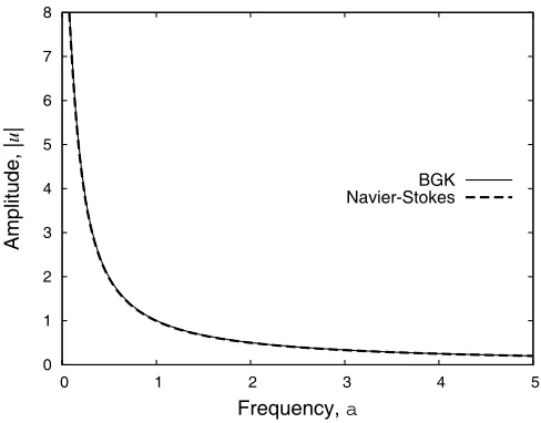
The quasi-steady case

We first consider a quasi-steady wave, i.e. =0. Figure 1 shows the amplitude of the shear wave,

super-Burnett and Grad’s 13 moment equations in as much as [they] … keep the desirable features of both”.

Time-varying shear waves

While our results for the quasi-steady case show that, for Kn≈0.1, the Navier-Stokes and the BGK models agree, we should extend the analysis to the time-dependent case. Figures 2 and 3 show that, for fixed Kn=0.1, the BGK model results closely match the Navier-Stokes solution for all frequencies considered, both in amplitude and phase lag. There does not, then, appear to be an independent non-equilibrium effect introduced by the body forcing frequency at low Kn.

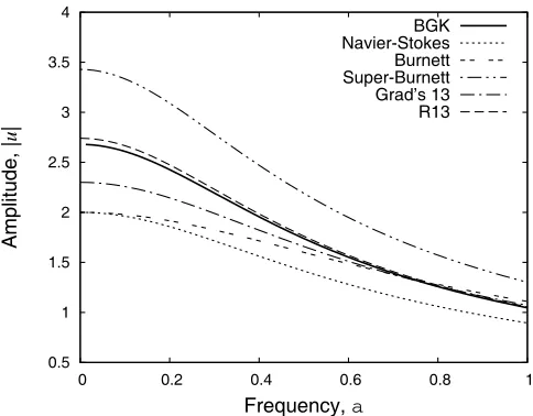
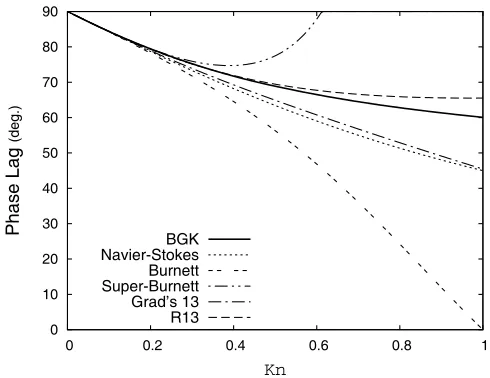
However, the form of the high-order continuum equations suggests that there may be non-equilibrium effects introduced by time-dependency at higher Kn. Figures 4 and 5 show results for the wave amplitude and phase lag, respectively, at a fixed Kn=0.5. In the case of the wave amplitude, the Navier-Stokes equations appear to be no better or worse at higher frequencies — the proportional difference between the Navier-Stokes and BGK results remains relatively constant. The BGK model predicts that non-equilibrium effects tend to make the shear wave lag behind the driving force. In both figures it is striking that the Burnett and super-Burnett results are quite poor, whereas the R13 equations accurately reproduce the BGK results over the range of frequencies considered.

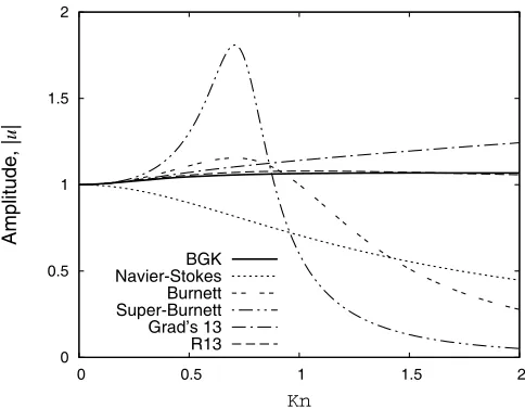
Our final set of standing shear wave results are for a fixed frequency oscillation, =1.0. Figures 6 and 7 show the wave amplitude and phase lag variation over a range of Kn. It is interesting to note that Figure 6 shows the BGK model predicts a slight increase in amplitude with increasing Kn, which is qualitatively different behaviour to the quasi-steady case. Again, the Burnett and super-Burnett equations are seemingly non-physical at higher Kn, whereas the R13 equations provide sensible and accurate results over a wide range of Kn.

Note that our analysis and results in this section, for a standing shear wave, are equivalent to those for a travelling shear wave of speed α . In that case, the non-dimensional body force, velocity response, shear stress, and heat flux would be F_x =ei(y+αt), u =uei(y+αt), τ_xy =τ_xyei(y+αt), and

) (y t i x

x q e

q = +α , respectively. The remainder of the analysis then follows identically, as do the results.

3. Knudsen layers

While the standing shear wave problem provides both a good illustration of non-equilibrium arising in a micro flow, and a simple test example for competing sets of high-order equations, any practical application of non-equilibrium flow models needs also to be able to capture the nonlinear stress/strain-rate behaviour within the Knudsen layer, as we outlined in section 1. The Knudsen layer is also an interesting problem because, while its structure has been extensively investigated and is well-understood from a kinetic theoretical viewpoint (see, e.g., Kogan 1969; Cercignani 1990; Sone 2002), high-order continuum equations generally have difficulties in predicting the extent of the layer — which kinetic theory predicts is some 1.4 molecular mean free paths into the flow from any surface. For example, the R13 equations, which performed well for the standing shear wave problem in section 2, predict a Knudsen layer of around twice this extent (see Lockerby et al. 2005a). There are also difficulties that arise in selecting the additional wall boundary conditions required for uniquely solving higher-order equations sets (although the recent work of Struchtrup & Torrilhon 2007 shows significant advances in this area).

3.1 Continuum-fluid models of slip

Integral to any calculation of the Knudsen layer is the model for gas slip at the surface. Maxwell’s (1879) slip boundary condition relates velocity slip to the shear stress at a gas-surface interface. Although his derivation was crude in comparison to modern kinetic theory, this boundary condition performs surprisingly well. It is partly owing to this, and its simplicity, that it still endures in rarefied gas dynamics (see Lockerby et al. 2004). This boundary condition, for isothermal cases, has the form:

μ τ λ σ

σ

− − = 2

slip

u , ₍₁₈₎

where uslip is the velocity slip, τ is the shear stress, μ is the viscosity, σ is the tangential momentum accommodation coefficient (equal to one for perfectly diffuse molecular deflection, and zero for purely specular deflection) and λis the mean free path, defined as:

p ρ π μ λ

2

= , (19)

where is the density, and p is the pressure.

However, one of the main shortcomings of Maxwell’s boundary condition is its inability to take into account the nonlinear stress/strain-rate relationship characteristic of the Knudsen layer (as depicted schematically in Figure 8). As a way of compensating for this, modern slip boundary conditions (see, e.g., Kogan 1969; Cercignani 1990; Sone 2002) use slip coefficients that predict greater than the actual slip at the boundaries. This ‘fictitious’ slip, as it is sometimes called, ensures that the linear Navier-Stokes model is accurate beyond the Knudsen layer, but not within it (i.e. the diagonal dashed line in Figure 8).

The Maxwell condition is often supplemented by a second-order contribution to the slip, i.e.

2 2 2 2 1

d d d

d

x u A x u A

u_slip = λ + λ , (20)

where x is in a direction normal to, and away from, the surface, and A1 and A2 are slip coefficients. Cercignani (1990) and others have calculated the values of these slip coefficients from numerical solutions to the BGK Boltzmann equation. For a monatomic and isothermal gas at low Knudsen number:

A1=1.1466 and A2= –0.9576, (21)

(this further assumes perfectly diffuse reflection of molecules at surfaces, i.e. =1).

Using the same DVM for the BGK Boltzmann model that we used in section 2.2, we compare in Figures 9 and 10 BGK solutions for isothermal Couette and Poiseuille channel flows with Navier-Stokes solutions using the boundary conditions (20) with (21). These results are for Kn(= /H)=0.05, where the characteristic length, H, is the channel depth. As expected, a near-precise agreement is shown; it is only near to the walls that any inaccuracy is evident. Note that all the results that follow are non-dimensionalised using , and p, all of which are constant for the cases presented.

If the average error in the Navier-Stokes velocity profile compared to the BGK result may be defined as:

(

)

2

max err

1

i BGK i BGK

u

u

u

u

=

−

, ₍₂₂₎

solutions is trivial. However, for complex geometries, such as those common in 3D microfluidic device design, the difference in computational requirements would be considerable.)

However, the accuracy of Navier-Stokes slip solutions rapidly diminishes at higher Knudsen numbers. For example, at Kn=0.5 the average errors in the Couette and Poiseuille flow slip solutions are 10% and 33%, respectively. So it is clear that there is a relatively low Knudsen number limit up to which the Navier-Stokes model with slip boundary conditions can be confidently applied.

The two fundamental problems with using ‘fictitious’ slip boundary conditions with the Navier-Stokes constitutive relations are: (a) that some portion of the flow domain is therefore necessarily fictitious, and at transitional Knudsen numbers (i.e. Kn=0.1~1), where the Knudsen layers are relatively much larger, this error becomes unacceptable; (b) that for moderate transitional Kn, the linear stress/strain-rate relationship is invalid, not just near the walls, but for the entire channel. For example, a BGK solution of Couette flow with Kn=0.5 shows that nowhere in the flow are the linear Navier-Stokes constitutive relations less than 16% inaccurate. This inaccuracy is inherent in the foundational axioms of linearity of the Navier-Stokes constitutive relations, and is irrespective of the amount of slip introduced at the boundary.

However, we here propose an adaptation to the Navier-Stokes model capable of addressing both of these problems. This new model has two components: micro slip coefficients, which model the actual slip at gas-surface interfaces; and a wall-distance-dependent scaling of the Navier-Stokes constitutive relations. It is important to stress that our new model, for rarefied monatomic gas flows, is calibrated with precisely the same BGK result as used in the generation of the standard second-order slip boundary conditions (20) with (21). Any generality is therefore left intact.

3.2 Near-wall scaling of the constitutive relations

For ease of implementation, we seek a simple functional relationship between the departure from Navier-Stokes behaviour and the wall-normal distance from a surface. This concept is similar to the “wall-function” proposed in Lockerby et al. (2005b). However, there are some marked differences in the model we propose below, most notably the presence of a second-order contribution to the near-wall scaling (second-order, in that it is dependent on a local Knudsen number) and a more accurate functional form (we also do not continue to use the phrase “wall-function” in the present paper, to avoid confusion with those wall-functions associated with turbulence modelling). There are some similarities between our method and effective viscosity approaches, such as the one proposed by Guo

et al. (2007).

For a simple 1D flow, we propose scaling the stress/strain-rate relationship as follows (the scaling for a 3D flow is essentially similar, see equations 31 to 34 below):

[

1

(

ˆ

)

(

ˆ

)

]

d

d

2

1

x

k

x

x

u

₌

₋

₊

_Ψ

₊

_Ψ

μ

τ

, (23)

with the functions Ψi defined by:

x c b

e x a

x _i ˆ

i

i i

ˆ ) ˆ

( =

Ψ , (24)

where is the perpendicular distance from a wall surface (nondimensionalised with ) and positive in the direction away from the surface; a

xˆ

i, bi and ci are coefficients to be determined; and the variable k

is:

x

k

ˆ

d

d

1

τ

τ

=

. (25)

suggesting that a positive (or negative)strain-rate might be possible in the presence of a positive (or negative) stress. This qualitatively non-Newtonian behaviour will be examined below.

Values for the coefficients ai, bi and ci are optimised using a simple genetic algorithm to most accurately reproduce the two low-Kn BGK results presented in Figures 9 and 10, resulting in:

a1 = 0.1859, b1= –0.4640, c1= –0.7902;

a2 = 0.4205, b2= –0.3518, c2= –0.4521. (26)

Although these values are given to four significant figures, our results that follow are reasonably insensitive to their exact values. For example, for a Poiseuille flow of Kn=0.2 (based on channel depth), a 5% alteration in any of the values listed in equations (26) results in less than 1% difference in the additional mass flow rate that occurs in the rarefied case.

Our scaling may be implemented conveniently within an existing computational fluid dynamics (CFD) code by defining a variable viscosity to effect the desired scaling. It is important to emphasize, however, that nothing artificial is being introduced into the subsequent Navier-Stokes calculations. The actual viscosity remains unaltered. Furthermore, the velocity profile correction that results is not at the expense of an inaccuracy in the prediction of stress (as will be demonstrated later); it is only the stress/strain-rate relationship that is being altered, and this is a reflection of what happens in reality.

The functional form given in equation (24) is qualitatively different to that proposed by Lockerby

et al. (2005b) and Guo et al. (2007), and has been chosen to more accurately reproduce the Knudsen layer’s actual structure; it allows for an indefinitely steep profile in the most inner regions of the Knudsen layer, and a more gradual decay in the outer regions. It also allows for a second-order contribution to the Knudsen layer. Interestingly, our model predicts an infinite scaling at the wall (since the coefficients b1 and b2 are negative), and therefore an infinite rate of strain. Although this might, at first, seem counter-intuitive, it is in accord with kinetic theory analysis of the Knudsen layer by Sone (2002). In practice, this has limited consequences on the implementation of our method since the function is evaluated within the first fluid cell close to a wall (i.e. between the surface and first fluid grid points). As such, there is no singularity to reckon with in the computational scheme. Difficulties only arise if the spatial resolution is particularly high; then derivatives become large and the errors associated with their evaluation significant. To avoid this, very near-wall scaling values (e.g. <0.05) can be obtained by linear extrapolation from a value that is close to the wall but which does not have excessively large derivatives (an example of this technique is discussed below).

xˆ

3.3 Combined effect of two parallel walls

At transitional Knudsen numbers it is likely that surfaces in close proximity will have a coupled effect on the departure of the flow from Navier-Stokes behaviour. Here, as an initial model, we assume that in parallel wall cases their contributions can be combined linearly. This rather crude assumption is based on the simple premise that the direct influence of a wall is restricted to molecules travelling away from its surface. Since, in steady flow cases, this set of molecules is half the total number, the opposite wall’s influence can be considered separately, and therefore added to this. In cases involving parallel walls the combined scaling function is then:

[

1 (ˆ ) (ˆ ) (ˆ ) (ˆ )

]

d

d

2 2

1

1 xa xb ka xa kb xb

x

u_{=− +Ψ +Ψ + Ψ + Ψ}

μ

τ _,

(27) where and are the distances measured normal to the first and second wall surfaces, respectively. It is important to note that this would make no appreciable difference to the low-Knudsen-number cases in Figures 9 and 10 because of the relatively large distance between the solid surfaces. It is highly likely that for non-planar cases this linear combination of Knudsen layer effects will need to be reconsidered in a more rigorous manner.

a

xˆ xˆ_b

In our new model we aim to model the actual (sometimes referred to as ‘micro’) slip, as opposed to a fictitious value of slip. So we propose here boundary conditions for the micro slip in a similar form to those used for fictitious slip, as in equation (20), but in terms of stress rather than strain-rate. For ordinary Navier-Stokes simulations this difference is of no consequence, but this is not the case for our model. Lockerby et al. (2004) showed that Maxwell’s slip boundary condition should be expressed in terms of stress rather than strain-rate, and so here we extend this to second order:

x A A

u_slip

d d 2

2 1

τ μ λ μ

τ

λ −

−

= . (28)

We obtain the values of the slip coefficients A1 and A2 directly from the low-Kn BGK solutions presented in Figures 9 and 10:

A1=0.798 and A2= –0.278. (29)

This completes our micro-slip Navier-Stokes model with near-wall scaling of the constitutive relations.

3.5 Results and comparison with a kinetic theoretical model

We now compare our new model to both conventional second-order slip solutions and BGK results at transitional Knusden numbers. This represents a real test of both the conventional second-order slip model (equation 20) and our new model, since both are based upon the same low-Kn BGK data.

It is important to be clear that we are not investigating the appropriateness of the physical model underpinning the BGK Boltzmann equation itself; we are only interested in whether the standard and our current models can achieve the same predictions. As such, we do not present solutions to the Boltzmann equation for the same test cases; however such solutions can be used to refine the calibration of our proposed model. Although not used in our simulations presented here, the model coefficients for a hard-sphere gas (calibrated using the data of Ohwada et al. 1989a,b) are: a1 = 0.1824;

b1= –0.5101; c1= –1.051; a2 = 0.2001; b2= –0.7193; c2= –0.652; A1=0.8055; and A2= –0.1452. The first-order coefficients (A1, a1, b1, c1) are very similar to those from the BGK model; the disparity in the second-order coefficients (A2, a2, b2, c2) reflects the inaccuracy of the BGK model unless adjusted to be applicable to hard spheres (Hadjiconstantinou 2003).

The results that follow are non-dimensionalised using , and p, all of which are constant for the cases presented (e.g. velocity is non-dimensionalised using

λ

p/

μ

, and shear stress using p). The simulations conducted here are trivial in terms of computational requirements, and far more numerical grid points have been used than necessary for an acceptably accurate result; all simulations in this section have been performed using 4000 grid points. To give an indication of grid dependency using our model, for Poiseuille flow (Kn=λ/H=0.1), 50 grid points provide a prediction of mass flow rate within 2% of that obtained using 5000 grid points.

Couette flow

Figure 11 shows the velocity profiles for a high-Kn Couette flow (Kn=λ/H=1.0) predicted by our new model, the standard slip model, and the BGK equation; the opposing non-dimensional wall velocities are equal to –1 and 1. Our model provides strikingly close agreement to this BGK solution. Figure 12 shows the average velocity error (defined in equation 22) for the no-slip solution, the slip solution, and our model over a range of Knudsen numbers. The slip solution has an average error of approximately 1% for Kn=0.07, whereas our model can reach Kn=2.0 before showing the same level of error; this clearly represents a significant extension of applicability of the continuum-fluid model.

Clearly, both the slip model and our current model very accurately predict the stress in the channel. For a Knudsen number as high as Kn=2.0 the stress predictions are within 5% of the BGK solution for our model and within 6% for the slip model.

Poiseuille flow

The second-order elements of the slip model and our current model are not tested in Couette flow, as it is a constant-stress problem. So we now consider planar Poiseuille flow at transitional Knudsen numbers. For these simulations we have chosen a non-dimensional streamwise pressure gradient equal to Kn.

Figure 14 shows the velocity profiles for a high-Kn Poiseuille flow (Kn=λ/H=1.0) predicted by our model (with the same coefficients, equations 26), the slip model and the BGK code. The current model provides a great improvement on the slip solution: the strain-rate variation of the velocity profile predicted by our model is very close to that of the BGK solution, suggesting that in this case it is the micro slip coefficient that is introducing most of the error, rather than the scaling of the constitutive relations.

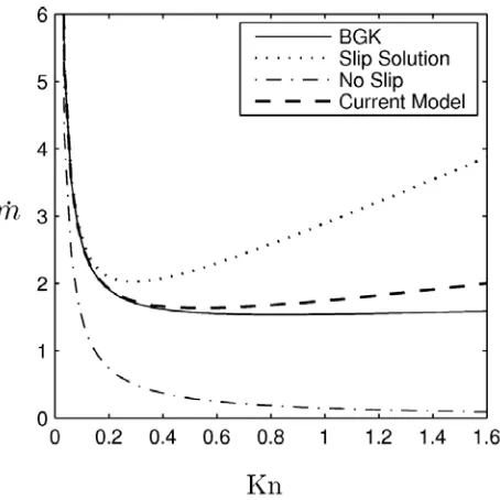
The average error of the velocity profile is plotted in Figure 15 for Knudsen numbers up to 2.0. The slip model shows an average error of 5% at a Knudsen number as low as 0.13, whereas our model can reach Kn=0.62 before showing the same average error. Our model’s improvement on the slip solution is therefore marked; this is reinforced by Figure 16, which shows predicted normalized mass flow rates for Knudsen numbers up to 1.6 for the various models and the BGK code. The ‘Knudsen minimum’ in the flow rate is captured much more accurately with our model as compared to the slip solution, although this minimum does appear to occur at a significantly lower Knudsen number (Kn~0.4) than the BGK model predicts (Kn~0.9). (Note that in this figure the Knudsen minimum appears quite slight; it would be more accentuated if the graph was extended to higher Kn.)

Couette/Poiseuille flow

In developing slip models and extensions to Navier-Stokes solvers, the hope is that they might be applicable to general geometries. The model we have proposed is no less general in its derivation than the conventional slip model we have used for comparison. An investigation into both models’ accuracy in cases other than Couette and Poiseuille flows is therefore required.

For a combined Couette/Poiseuille test case we have chosen a non-dimensional pressure gradient equal to Kn and opposing wall velocities equal to –1 and 1. Figure 17 shows the velocity profile of this combined flow at Kn=1.0. Again, our current model (with the same coefficients) provides a much better prediction than the conventional slip model. The average error of the velocity profile is plotted in Figure 18 versus Knudsen number. The slip model shows a 5% average error at a Knudsen number of 0.14, whereas our model can reach a Knudsen number of 0.67 before showing the same level of error.

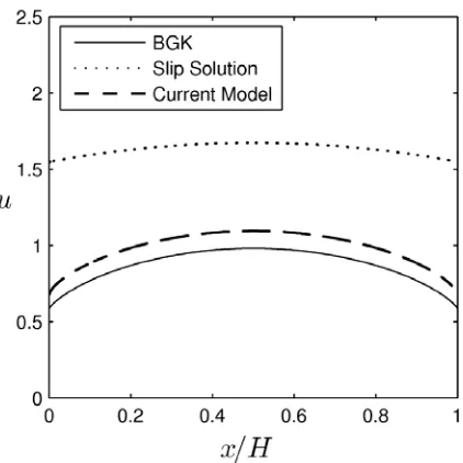
It was mentioned in section 3.2 that our model might predict regions of positive (or negative) strain-rate that are coincident with positive (or negative) shear stress. This qualitatively non-Newtonian behaviour is noticeable in Figure 17. The shear stress in the entire flow is negative, and consequently, the Navier-Stokes slip solution predicts a positive rate of strain throughout the channel. However, the BGK solution clearly predicts an inversion in the rate of strain at x>0.85H; an unexpected phenomenon, but captured by our new model quite well.

3.6 Results and comparison for micro-sphere flow

The oil droplet experiments of Millikan (1923) demonstrated that the classical Stokes drag prediction of flow past a sphere needed correcting as the Knudsen number increased. Allen & Raabe (1985) conducted a similar but improved experiment and used their data to obtain a drag formula, dependent on Knudsen number (based on sphere radius), as follows:

(

_/

)

1

(

1+ + − −

= Kn

S Kn e

D

D

α

β

γ , (30)

where Ds is the Stokes drag, Kn is the Knudsen number based on sphere radius, α=1.142 ± 0.0024, β =0.558 ± 0.0024, and γ =0.999 ± 0.0212. This expression will be used as our experimental benchmark to which we compare the predictions of our model, alongside conventional slip solutions.

The governing equations

The 3D low-speed incompressible Navier-Stokes momentum equations with our constitutive-relation scaling are as follows:

(

U

)

U U

P= ∇⋅ Φ∇ = Φ∇ + ∇Φ⋅∇

∇ 2μ μ 2 2μ , (31)

where

( )

[

T

]

U U

U = ∇ + ∇

∇

2 1

, (32)

and

[

]

1

2 1(ˆ) (ˆ)

1+Ψ + Ψ −

=

Φ n k n , (33)

with being the non-dimensional surface-normal distance from the nearest wall surface, and the functions Ψ

nˆ

i and their coefficients are, again, those in equations (24) to (26). The variable k is

calculated as follows:

n

k

ˆ

d

d

1

τ

τ

=

, with

τ

=i_xˆ⋅(i_nˆ ⋅ ), (34)

where is the stress tensor, is a unit vector in the wall-normal direction and is a unit vector perpendicular to in a direction that gives maximum shear stress, τ. Our constitutive-scaling model as a whole can indirectly (although will not necessarily) affect the shear stress field, which in turn will alter k, producing a weak coupling effect.

n

iˆ ixˆ

nˆ

A schematic of the sphere and the coordinate system adopted is shown in Figure 19. The symmetry of the problem indicates a solution independent of θ, and with no θ-component of velocity, i.e.

⎥

⎥

⎥

⎦

⎤

⎢

⎢

⎢

⎣

⎡

=

0

φ

U

U

U

r

;

=

0

∂

∂

=

∂

∂

=

∂

∂

θ

θ

θ

φ

p

U

U

_r

. (35)

Furthermore, since this is creeping flow (i.e. very low Reynolds number), variations in flow variables can be assumed to have the following form, with dependence only on r:

φ

φ

) ( )cos ,

(r u r

U_r = _r ,

φ

φ

_φ

φ(r, ) u (r)sin

U = ,

φ

φ

) ( )cos ,

(r p p r

P = _∞ + ,

(36)

where p_∞is the free-stream pressure.

The continuity and momentum equations are then:

r

U

U

r

r

U

r

U

_{r r}

φ

φ

φ φ

cot

1

2

0

+

∂

∂

+

+

∂

∂

⎟⎟ ⎠ ⎞ ⎜⎜ ⎝ ⎛ − ∂ ∂ − ∂ ∂ + ∂ ∂ + − ∂ ∂ + ∂ ∂ Φ = ∂ ∂ 2 2 2 2 2 2 2 2

2 _{2 cot}

2 cot 1 2 2 r U U r U r U r r U r U r r U r

P _{r r r r r}

φ

φ

φ

φ

φ

μ

φ φ

r

U

r

r

∂

∂

∂

Φ

∂

+

μ

,

(38) ⎟ ⎟ ⎠ ⎞ ⎜ ⎜ ⎝ ⎛ ∂ ∂ + ∂ ∂ + ∂ ∂ + − ∂ ∂ + ∂ ∂ Φ = ∂ ∂

φ

φ

φ

φ

φ

μ

φ

φ φ φ φ

φ Ur

r U r U r r U r U r r U P

r 2 2 2

2 2 2 2 2 2 2 cot 1 sin 2 1 ⎟⎟ ⎠ ⎞ ⎜⎜ ⎝ ⎛ − ∂ ∂ + ∂ ∂ ∂ Φ ∂ + r U U r r U r r φ φ

φ

μ

1 .

(39)

Note that

Φ

has dependence only on r, which is equal to

λ

nˆ (the variable k, which needs to be evaluated for

Φ

, is also dependent only on r despite the shear stress, τ , varying with sinφ). After making substitutions for U_r, U_φ and P given in equations (36), and after eliminating ur from the momentum equations, equations (37) to (39) become:

dr

du

r

u

u

r r

2

−

−

=

φ , (40)

dr du dr d dr du r dr u d dr

dp _{r r} Φ _r

+ ⎟⎟ ⎠ ⎞ ⎜⎜ ⎝ ⎛ + Φ

=

μ

₂ 4 2

μ

2 , (41) ⎟⎟ ⎠ ⎞ ⎜⎜ ⎝ ⎛ + Φ + ⎟⎟ ⎠ ⎞ ⎜⎜ ⎝ ⎛ + + Φ = dr du dr u d r dr d dr du r dr u d dr u d r r

p _{r r r r r}

2 2 2 2 3 3 2 2 3 2

μ

μ

. (42)

Then differentiating equation (42) and substituting into equation (41) (to eliminate pressure) gives the following fourth-order ordinary differential equation:

⎟⎟ ⎠ ⎞ ⎜⎜ ⎝ ⎛ + + Φ + ⎟⎟ ⎠ ⎞ ⎜⎜ ⎝ ⎛ − + + Φ = dr du dr u d r dr u d r dr d dr du r dr u d dr u d r dr u d

r _{r r r r r r r}

2 2 3 3 2 2 2 3 3 4 4 2 5 4 4 4 2 0 ⎟⎟ ⎠ ⎞ ⎜⎜ ⎝ ⎛ + Φ + dr du r dr u d r dr

d _{r r}

2 2 2 2 2 2 . (43)

This is solved with the following boundary conditions:

∞

= ∞

= U

r

ur( ) ,

0 ) (r =a =

u_r ,

0

)

(

r

=

∞

=

dr

du

_r ,

a

u

a

u

a

r

dr

du

r

₍

=

₎

=

−

2

φ

=

2

slip _,

(44)

where a is the radius of the sphere and is the free-stream velocity. Note that in the final boundary condition given in equations (44), the gradient of at the surface of the sphere is related to the slip velocity via the continuity equation (40).

∞

U

r

u

The surface shear stress, τ, and surface normal stress, σ, are as follows:

φ

τ

φ

τ

( )= ˆsin ,

σ

(

φ

)=

σ

ˆcos

φ

, (45)

where ⎟⎟ ⎠ ⎞ ⎜⎜ ⎝ ⎛ + Φ = dr du dr u d

r _{r r}

2 2

2

ˆ

μ

τ

,

⎟

⎠

⎞

⎜

⎝

⎛

Φ

−

=

dr

du

_r

μ

These expressions, combined with the pressure that is obtained from equation (42), can be used to evaluate the total drag force, F, on the sphere:

(

P

)

s

F

S

d

∫

+

−

=

σ

τ

, ₍₄₇₎

where S is the surface of the sphere and ds=a2sin

φ

d

φ

d

θ

. By substituting equations (45), and the pressure equation in equations (36), into equation (47) our final expression for the drag force is obtained:

(

σ

τ

)

π

ˆ

2

ˆ

3

4

2

₊

₋

=

a

p

F

. (48)

Note that, numerically, the surface stresses and surface pressure may be evaluated by one-sided finite differences.

Numerical procedure

The domain is semi-infinite, and so the following mapping is used:

L

a

r

L

+

−

=

η

, (49)

where

η

is the mapped variable (

η

=1 at the sphere surface,

η

=0 at infinity) and L is a scaling factor. The derivatives featuring in equation (43) can be rewritten in terms of

η

as follows:

⎟⎟

⎠

⎞

⎜⎜

⎝

⎛

∂

∂

−

≡

∂

∂

η

η

_r r

u

L

r

u

2 , ⎟⎟ ⎠ ⎞ ⎜⎜ ⎝ ⎛ ∂ ∂ + ∂ ∂ ≡ ∂ ∂

η

η

η

η

_{r r}

r u u

L r u 2 2 2 2 4 2 2 , ⎟⎟ ⎠ ⎞ ⎜⎜ ⎝ ⎛ ∂ ∂ + ∂ ∂ + ∂ ∂ − ≡ ∂ ∂

η

η

η

η

η

η

_{r r r}

r u u u

L r u 2 2 2 3 3 3 6 3 3 6 6 , ⎟⎟ ⎠ ⎞ ⎜⎜ ⎝ ⎛ ∂ ∂u + ∂ ∂ + ∂ ∂ + ∂ ∂ ≡ ∂ ∂

η

η

η

η

η

η

η

_{r r r r}

r u u u

L r u 3 2 2 2 3 3 4 4 4 8 4 4 24 36 12 . (50)

We discretise the resulting differential equation using centred finite differences and solve it using a standard linear equation solver. For all computations presented here, 4000 grid points have been used, but acceptably accurate results can be obtained with far fewer points. For Kn=0.1, a simulation with

η

100 grid points obtains a prediction of drag within 2.5% of that obtained using 4000 grid points; a simulation with 300 grid points, within 1%.

One minor numerical complication arises from the derivatives of the function tending to infinity at the surface of the sphere. To circumvent the numerical problems this causes, the function is linearly extrapolated back towards the surface for values of n<0.05. This extrapolated region is very small and has negligible effect on the solution other than to stabilise it.

ˆ

Results

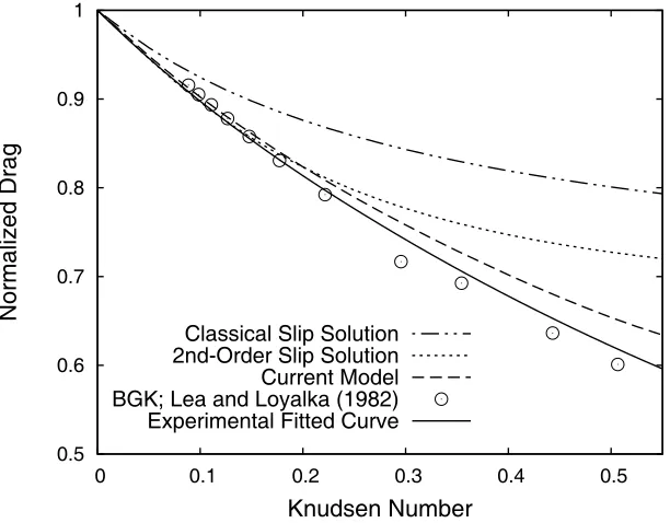
Our model is compared with the experimentally-fitted function of equation (30), a first-order slip olution due to Basset (1888) (A1=1; A2=0), a second-order slip solution given by Cercignani (1990) 66; A= 0.9576), and BGK results from Lea & Loyalka (1982). Our results for drag, s

(A1=1.14 2

normalized by Stokes’ continuum drag prediction (F=6πμaU∞), are shown in Figure 20.

slip

eded to establish whether this

f different continuum-type equations, each purporting to capture non-quilibrium physical flow effects, against a simple new benchmark case in rarefied flows: the time-vary

loped a new Navier-Stokes model for monatomic micro gas flow simu

edictions of drag, altho

effective

grid points are not required to maintain accuracy);

ar flows considered;

Fu

Knudsen layer that is important in non-isothermal flows;

collision

The t a well-documented DVM

ode that generated the BGK results presented in this paper. We also thank the referees of this paper model, when compared to both the experimental data and the BGK result. Considering that the second-order slip solution also has fictitious contributions to the flow velocity near to the wall (as we noted in section 3.1), our current model is therefore greatly to be preferred.

One caveat to this latter statement is that at much higher Kn (greater than about 0.6), and for this configuration, our model meets some stability problems. More work is ne

is a problem with the current implementation strategy, or an inherent instability in the model.

4. Discussion and conclusions

We have tested a number o e

ing standing shear wave. While this is an ideal case, it has the distinctive advantage of separating rarefied gas effects in the bulk flow from those due to solid bounding surfaces. Another advantage is that the analysis is relatively simple, so competing continuum-type models can be evaluated straightforwardly. We showed that the R13 equations, proposed by Torrilhon and Struchtrup as a development of Grad’s original 13 moment technique, provide the best model among those we tested. More complicated cases than this ideal benchmark may, however, require efficient computational methods in order to make the R13 equations a tractable design tool; it is unclear at present how computationally demanding calculations of 3D flows in complex geometries may be for any high-order continuum equation set.

To tackle, within the conventional fluid dynamics framework, the non-equilibrium introduced by solid surfaces we have deve

lations. This combines slip boundary conditions with a near-wall scaling of the constitutive relations. We showed that this model is much more accurate at higher Knudsen numbers than the conventional second-order slip model. It provides good results for combined Couette/Poiseuille flow, and can predict the stress-strain-rate inversion that is evident from BGK solutions.

We also applied our new model to the non-planar low-speed micro-flow around a sphere. Again, it demonstrated a marked improvement on conventional second-order slip pr

ugh there are some as yet unanswered questions regarding its stability at high Knudsen numbers. In addition to its predictive capabilities in planar and curved geometries, our new model

• does not require re-calibration of its coefficients for different geometries;

• is easily and consistently implemented within existing CFD frameworks as a scaled viscosity;

• is of equivalent computational cost to the standard Navier-Stokes equations (and additional numerical

• is based on the same BGK results as standard second-order slip boundary conditions, i.e. it has not been fitted to higher Knudsen number data for the particul

• does not require additional boundary conditions for higher moments of the flow properties. ture work should include:

• consideration of the effect of non-parallel wall interactions on the overall flowfield;

• incorporating the thermal

• developing micro slip and constitutive relation scaling based on a more sophisticated model than the BGK approximation;

• investigating polyatomic gas flows and the effect of gas mixtures.

au hors would like to thank Prof Dimitris Valougeorgis for providing c

REFERENCES

Allen, M. D. & Raabe, O. G. 1985 Slip cor ents of spherical solid aerosol-particles in and improved Millikan apparatus. Aerosol Sci. Tech. 4, 269-286.

Bu ean motion in a non-uniform gas.

Ch 0 The Mathematical Theory of Non-Uniform Gases, 3rd edn.

Gr 007 The structure of shock waves as a test of Brenner’s

Lea, K. C. & Loyalka, S. K. 1982 Motion of a sphere in a rarefied gas. Phys. Fluids 25, 1550.

elocity boundary condition at

surfaces. Phys. Rev.22, 1.

by pressure, temperature and concentration gradients. Phys.

Oh

parallel plates on the basis of the Boltzmann equation for hard-sphere

Oh

asis of the linearized Boltzmann equation for hard-sphere

Re

ynamic and microsystem flows. Phil. Trans. Roy. Soc. A361,2967.

Str

ent equations: derivation and rection measurem

Basset, A. B. 1888 A Treatise on Hydrodynamics, Cambridge University Press, Cambridge. rnett, D. 1935 The distribution of molecular velocities and the m

Proc. Lond. Math. Soc.40, 382.

Cercignani, C. 1990 Mathematical Methods in Kinetic Theory. Plenum Press, New York. apman, S. & Cowling T.G. 197

Cambridge University Press.

Grad, H. 1949 On the kinetic theory of rarefied gases. Commun. Pure Appl. Math.2, 331. eenshields, C. J. & Reese, J. M. 2

modifications to the Navier-Stokes equations. J. Fluid Mech.580, 407.

Guo, Z. L., Shi, B. C. & Zheng, C. G. 2007 An extended Navier-Stokes formulation for gas flows in the Knudsen layer near a wall. EPL80, 24001.

Hadjiconstantinou, N. 2003 Comment on Cercignani's second-order slip coefficient. Phys. Fluids 15, 2352

Kogan, M. N. 1969 Rarefied Gas Dynamics. Plenum Press, New York. Lockerby, D. A., Reese, J. M., Emerson, D. R. & Barber, R. W. 2004 V

solid walls in rarefied gas calculations. Phys. Rev. E70, 017303.

Lockerby, D. A., Reese, J. M. & Gallis, M. A. 2005a The usefulness of higher-order constitutive relations for describing the Knudsen layer. Phys. Fluids17,100609.

Lockerby, D. A., Reese, J. M. & Gallis, M. A. 2005b Capturing the Knudsen layer in continuum-fluid models of nonequilibrium gas flows. AIAA J. 43, 1391.

Maxwell, J. C. 1879 On stresses in rarefied gases arising from inequalities of temperature. Phil. Trans. Roy. Soc. London170, 231.

Millikan, R. A. 1923 The general law of fall of a small spherical body through a gas, and its bearing upon the nature of molecular reflection from

Naris, S. & Valougeorgis, D. 2005 The driven cavity flow over the whole range of the Knudsen number. Phys. Fluids17, 907106.

Naris, S., Valougeorgis, D., Kalempa, D. & Sharipov, F. 2005 Flow of gaseous mixtures through rectangular microchannels driven

Fluids17, 100607.

wada, T., Sone Y. & Aoki, K. 1989a Numerical analysis of the Poiseuille and thermal transpiration flows between two

molecules. Phys. Fluids A1(12) , 2042.

wada, T., Sone Y. & Aoki, K. 1989b Numerical analysis of the shear and thermal creep flows of a rarefied gas over a plane wall on the b

molecules. Phys. Fluids A1(9), 1588.

ese, J. M. 1993 On the structure of shock waves in monatomic rarefied gases. PhD thesis, Oxford University, UK.

Reese, J. M., Gallis, M. A. & Lockerby, D. A. 2003 New directions in fluid dynamics: non-equilibrium aerod

Sone, Y. 2002 Kinetic Theoryand Fluid Dynamics. Birkhauser, Boston.

uchtrup, H. 2005 Macroscopic Transport Equations for Rarefied Gas Flows. Springer. Struchtrup, H. & Torrilhon, M. 2003 Regularization of Grad’s 13-mom

Struchtrup, H. & Torrilhon, M. 2007 H theorem, regularization, and boundary conditions for linearized 13 moment equations. Phys. Rev. Lett.99, 014502.

Va e discrete velocity method: gaseous

Valougeorgis, D. 1988 Couette flow of a binary gas mixture. Phys. Fluids31, 521. lougeorgis, D. & Naris, S. 2003 Acceleration schemes of th

0 2 4 6 8 10

0.1 0.2 0.3 0.4 0.5 0.6 0.7 0.8 0.9 1

Amp

lit

u

d

e

,

|

u

|

Kn

[image:18.595.172.414.97.285.2]

BGK Navier-Stokes; Burnett Super-Burnett Grad’s 13 R13

Figure 1. Quasi-steady wave amplitude variation with Knudsen number. BGK solution ( ); Navier-Stokes and Burnett (···); super-Burnett ( · · ); Grad’s 13 moment ( · ); Regularized 13 moment ( ).

0 1 2 3 4 5 6 7 8

0 1 2 3 4 5

Amp

lit

u

d

e

,

|

u

|

Frequency, a

BGK Navier-Stokes

[image:18.595.172.416.412.603.2]

0 10 20 30 40 50 60 70 80 90

0 1 2 3 4 5

Ph

a

se

L

a

g

(d

e

g

.)

Frequency, a

[image:19.595.171.419.82.274.2]

BGK Navier-Stokes

Figure 3. Velocity phase lag variation with non-dimensional body force frequency, ; Kn=0.1; BGK solution ( ); Navier-Stokes ( ).

0.5 1 1.5 2 2.5 3 3.5 4

0 0.2 0.4 0.6 0.8 1

Amp

lit

u

d

e

,

|

u

|

Frequency, a

BGK Navier-Stokes Burnett Super-Burnett Grad’s 13 R13

[image:19.595.173.415.382.571.2]

0 10 20 30 40 50 60 70 80 90

0 1 2 3 4 5

Ph

a

se

L

a

g

(d

e

g

.)

Frequency, a

[image:20.595.171.418.82.274.2]

BGK Navier-Stokes Burnett Super-Burnett Grad’s 13 R13

Figure 5. Velocity phase lag variation with non-dimensional body force frequency, ; Kn=0.5. BGK solution ( ); Navier-Stokes (···); Burnett ( ); super-Burnett ( · · ); Grad’s 13 moment ( · ); Regularized 13 moment ( ).

0 0.5 1 1.5 2

0 0.5 1 1.5 2

Amp

lit

u

d

e

,

|

u

|

Kn

BGK Navier-Stokes Burnett Super-Burnett Grad’s 13 R13

[image:20.595.173.415.397.585.2]

0 10 20 30 40 50 60 70 80 90

0 0.2 0.4 0.6 0.8 1

Ph

a

se

L

a

g

(d

e

g

.)

Kn

[image:21.595.171.416.83.272.2]

BGK Navier-Stokes Burnett Super-Burnett Grad’s 13 R13

Figure 7. Velocity phase lag variation with Knudsen number; =1.0. BGK solution ( ); Navier-Stokes (···); Burnett ( ); super-Burnett ( · · ); Grad’s 13 moment ( · ); Regularized 13 moment ( ).

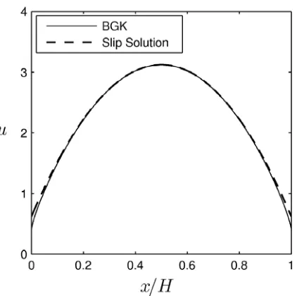
[image:21.595.205.369.395.553.2]

[image:22.595.193.416.78.294.2]

Figure 9. Non-dimensional velocity profile for Couette flow, Kn=0.05 (=λ/H). Comparison of the BGK solution (–) with the slip solution (– –). Non-dimensional wall velocities at x=0and x=H are –1 and 1, respectively.

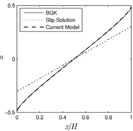
[image:22.595.193.404.420.630.2]

[image:23.595.186.402.81.294.2]

Figure 11. Non-dimensional velocity profile for high Knudsen number Couette flow (Kn=1.0). Comparison of the slip solution (···), the BGK solution (–), and our model (– –). Non-dimensional wall velocities at x=0and x=H are –1 and 1, respectively.

[image:23.595.186.410.422.639.2]

[image:24.595.186.407.80.296.2]

Figure 13. Non-dimensional Couette flow shear stress up to Kn=1.0. Comparison of the no-slip solution (– ·), slip solution (···), and our model (– –). The non-dimensional wall velocities at x=0and

x=H are –1 and 1, respectively.

[image:24.595.192.403.419.630.2]

[image:25.595.182.415.84.296.2]

Figure 15. Average error of Poiseuille flow velocity predictions up to Kn=2.0. Comparison of no-slip solution (– ·), slip solution (···), and our model (– –). The non-dimensional applied pressure gradient is Kn.

[image:25.595.184.411.429.656.2]

[image:26.595.195.409.85.302.2]

Figure 17. Non-dimensional velocity profile for high-Knudsen-number combined Couette/Poiseuille flow (Kn=1.0). Comparison of the slip solution (···), the BGK solution (–), and our model (– –). The non-dimensional applied pressure gradient is Kn, and the non-dimensional wall velocities at x=0 and

x=H are –1 and 1, respectively.

[image:26.595.179.415.436.653.2]

[image:27.595.224.375.92.288.2]

Figure 19. Coordinate system for the micro-sphere flow problem.

0.5 0.6 0.7 0.8 0.9 1

0 0.1 0.2 0.3 0.4 0.5

N

o

rma

lize

d

D

ra

g

Knudsen Number Classical Slip Solution 2nd-Order Slip Solution Current Model BGK; Lea and Loyalka (1982) Experimental Fitted Curve

[image:27.595.141.447.364.603.2]