What If ? Robust Prediction Intervals for Unbalanced Samples

W

HAT

I

F

…?

R

OBUST

P

REDICTION

I

NTERVALS FOR

U

NBALANCED

S

AMPLES

R.

L.

C

HAMBERS

A

BSTRACT

A confidence interval is a standard way of expressing our uncertainty about the value of a

population parameter. In survey sampling most methods of confidence interval estimation rely

on “reasonable” assumptions to be true in order to achieve nominal coverage levels. Typically

these correspond to replacing complex sample statistics by large sample approximations and

invoking central limit behaviour. Unfortunately, coverage of these intervals in practice is

often much less than anticipated, particularly in unbalanced samples. This paper explores an

alternative approach, based on a generalisation of quantile regression analysis, to defining an

interval estimate that captures our uncertainty about an unknown population quantity. These

quantile-based intervals seem more robust and stable than confidence intervals, particularly in

unbalanced situations. Furthermore, they do not involve estimation of second order quantities

like variances, which is often difficult and time-consuming for non-linear estimators. We

present empirical results illustrating this alternative approach and discuss implications for its

use.

What If …. ? Robust Prediction Intervals for Unbalanced Samples

R. L. Chambers

Southampton Statistical Sciences Research Institute University of Southampton

Highfield

Southampton SO17 1BJ UK

Abstract

A confidence interval is a standard way of expressing our uncertainty about the value of a population parameter. In survey sampling most methods of confidence interval estimation rely on “reasonable” assumptions to be true in order to achieve nominal coverage levels. Typically these correspond to replacing complex sample statistics by large sample approximations and invoking central limit behaviour. Unfortunately, coverage of these intervals in practice is often much less than anticipated, particularly in unbalanced samples. This paper explores an alternative approach, based on a generalisation of quantile regression analysis, to defining an interval estimate that captures our uncertainty about an unknown population quantity. These quantile-based intervals seem more robust and stable than confidence intervals, particularly in unbalanced situations. Furthermore, they do not involve estimation of second order quantities like variances, which is often difficult and time-consuming for non-linear estimators. We present empirical results illustrating this alternative approach and discuss implications for its use.

1. Introduction

Confidence intervals are an integral part of modern statistical inference. The concept of an interval estimator for an unknown parameter value that includes this value a pre-specified proportion of the time under repeated sampling permeates virtually every branch of statistics. In survey sampling confidence intervals are routinely calculated as part of the survey estimation process, with the ubiquitous 95% or “2 standard error” interval serving to define what many users interpret as a “credible” interval for a target population quantity.

In large part, the validity of the “confidence” interpretation of confidence intervals in survey sampling rests on large sample approximations and consequent application of the central limit theorem. Typically these approximations seem reasonable. However, there is much empirical evidence, particularly from simulation experiments, that the nominal confidence levels ascribed to these intervals are often not achieved in practice. Why this is so is unclear in general, although it seems to be related to failure of central limit assumptions brought about by a combination of non-normal population structures (e.g. outliers, heavy-tailed distributions) and sampling methods that result in “unrepresentative” or “unbalanced” samples. Royall and Cumberland (1985) explored these issues in the context of an empirical study of ratio and regression estimation of population totals, using both conventional design-based variance estimators as well as robust model-design-based variance estimators to construct nominal 95% intervals using data from samples drawn from a number of real populations. Their results showed that in unbalanced samples all the interval estimation methods they considered had serious under-coverage problems. They also found instances (e.g. the Counties 70 population) where none of these intervals came anywhere close to their nominal level of coverage on any sample, irrespective of its balance.

As far as the author is aware, the situation today, some twenty years after the publication of Royall and Cumberland (1985), remains unchanged - confidence intervals are still routinely produced by survey statisticians using techniques that are basically the same as those investigated by these authors, and claims about nominal levels of coverage that cannot be guaranteed are still being made. We still do not know how to specify a confidence interval that lives up to its name. We make large sample approximations, invoke central limit behaviour and keep our fingers crossed.

The purpose of this paper is to suggest that the “traditional” approach to constructing a confidence interval, e.g. the sample value of an estimator plus or minus twice the sample estimate of its standard error, is not the only way one can systematically approach construction of interval estimates for unknown population quantities. There are other ways of defining intervals that capture our uncertainty about these quantities and seem more robust and stable than confidence intervals, particularly in unbalanced situations. Furthermore, these intervals do not involve estimation of second order quantities like the variances of estimators, which is often difficult and time-consuming, especially for non-linear estimators. Instead, they are defined by calculating fairly straightforward estimates for populations that our sample might have been drawn from. A drawback of such an approach is that the concept of guaranteed coverage no longer applies, being replaced instead by a measure of the potential differences between the “most likely” sampled population and reasonable alternatives that could also have given rise to the sample data.

extremely unbalanced. We show that efficient methods of estimation using these data do not lead to good confidence intervals and we explore some reasons for why this is the case. In Section 3 we then introduce an alternative method of interval estimation based on a generalisation of the idea of quantile regression modelling. We show that interval estimates produced using this approach are not only easy to calculate and interpretable, but also have robust coverage properties. In section 4 we then move on to a more complex non-linear estimation problem where methods of confidence interval estimation are extremely difficult to implement and also have very poor coverage properties. Here we show that the alternative quantile regression model intervals are simpler to calculate and have better coverage. Finally, in Section 5 we explore some areas for further research.

2. Constructing Prediction Intervals for Average Hourly Pay

The New Earnings Survey (NES) was a large-scale annual survey of employees in the UK business sector, carried out by the UK Office for National Statistics, that collected data on salaries, hours worked and hourly rates of pay. From 2004 the NES was replaced by the Annual Survey of Hours and Earnings (ASHE), which has essentially the same remit. We confine our analysis in this paper, however, to data collected in the 2002 round of NES, since data collected in ASHE are expected to be similar.

A key objective of NES was measurement of the hourly pay rates for all employees, denoted Y from now on. By definition, this variable cannot be obtained from all sampled employees since many are not paid by the hour. However, it is possible to calculate an implicit hourly rate (X = derived rate) based on total earnings and hours worked, both of which are available for all sampled employees. From Table 1 we see that the distributions of Y and X are not the same in the NES sample. Furthermore, X is generally not the same as Y when both are available, as can be seen in Table 2.

Table 1 Distribution of NES data for 2002 based on the total sample of 162,843 employees, of whom 75,850 provided hourly pay rate data (Y). All values are in pence.

Quantiles of distribution

Y available? 25% 50% 75%

Yes Y 482 597 843

X 492 634 892

[image:4.595.205.389.638.752.2]

No X 717 1014 1491

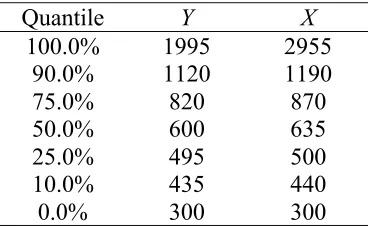
Table 2 Distributions of Y and X for the n = 59,590 employees that providing these values and satisfied 300 ≤Y ≤2000 and 300≤ X ≤3000. All values are rounded to nearest five pence.

Quantile Y X

100.0% 1995 2955

90.0% 1120 1190

75.0% 820 870

50.0% 600 635

25.0% 495 500

10.0% 435 440

[image:5.595.129.456.227.440.2]

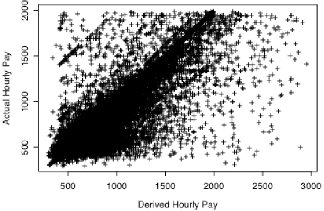
The employees contributing to Table 2 were restricted in terms of their values of Y and X to remove a large number of outliers in the NES data and to allow analysis to focus on that part of the pay rate distribution of most interest, corresponding to hourly pay rates between 400 and 1000 pence. A scatterplot of Y versus X for these employees is shown in Figure 1. Note the general “linearity” of the relationship between the two variables, as well as the large variability around this straight-line relationship. Notice also the impact of the UK minimum wage legislation, leading to a sharp drop in Y values below 400.

Figure 1 Scatterplot of observed hourly pay rate (Y) versus derived hourly pay rate (X) for the 59,590 employees in the NES sample with 300 ≤Y ≤2000 and 300≤ X ≤3000.

In what follows we use s1 to denote sample units (employees) that provide data for both Y and X and s2 to denote the remaining sample units that provide data for X alone. The overall sample is denoted s. Since the NES sample is essentially a simple random sample of all employees, the desired estimator of the mean hourly pay rate is

y_s =n−1 y_i

s1

∑

+ y_j

s2

∑

⎡

⎣ ⎤⎦.

However, as already pointed out, this statistic cannot be calculated. What can be done instead is to use the observed values of X to impute corresponding values of Y for those units where Y is “missing”. The above mean can then be calculated substituting imputed values of Y in the second summation term. From Figure 1 an obvious method of imputation (and one that has been shown to work well with these data) is simple regression imputation, based on a linear model linking Y and X. The imputed value of y_s is then equivalent to a regression estimator, where we treat s as the “population” of interest, with s1 defining the “sample”, and estimate the unobserved “population” mean y_s using the sample X values as auxiliary information. Furthermore, given the large number of “outliers” evident in Figure 1 it would seem sensible to use outlier robust methods of parameter estimation when calculating this regression estimate (or equivalently, constructing imputed values).

y_reg =n−1 y_i

s1

∑

+ (a_reg+b_regx_j) s2

∑

(

)

= n−1 w_i,regy_i

s1

∑

(1)

where

w_i,reg = n n₁ +n2

(xi −xs₁)(xs₂ −xs₁) (x_k −x_s

1)

2

s₁

∑

.

As noted earlier, the large variability in the Y-X relationship for those units where both of these variables are observed suggests use of a robust regression estimator, which in this case we write as

yrreg =n

−1

yi s₁

∑

+ _s (arreg+brregxj)

2

∑

(

)

=n−1 _s wi,rregyi

1

∑

(2)

where

w_i,rreg =1+ n2φi

φk s1

∑

1+

(x_i −x_φs

1)(xs2 −xφs1)

φk s1

∑

( )

−1

φk(xk−x_φs₁)

2 s1

∑

⎛ ⎝ ⎜ ⎜ ⎜ ⎞ ⎠ ⎟ ⎟ ⎟

x_φs

1 =

( )

∑

s₁φk

−1

φkxk s₁

∑

φi =

s_robψ

(

s_rob−1(y_i−a_rreg−b_rregx_i)

)

(y_i−a_rreg−b_rregx_i) .

Here s_rob is a robust estimate of the scale of the regression residuals and ψ denotes the influence function associated with the robust regression fit. In what follows we use the MAD estimate for s_rob and define ψ using the Huber specification

ψ(t)=t I(|t|≤c)+csgn(t)I(|t |>c)

with two choices of the tuning constant, c = 1.345 (default value, very robust, but not efficient) and c = 5 (not so robust, but more efficient). In practice computation of all these quantities is easily carried out using a modified version of function rlm (Venables and Ripley, 2002) in R (R Development Core Team, 2004).

In the context of model-based survey sampling, confidence intervals are prediction intervals or PIs. A large sample 95% PI for y_s based on the regression estimator is

y_reg±2 ˆV_reg

where Vˆ_reg is a robust estimate of the prediction variance of the regression estimator (Royall and Cumberland, 1981),

ˆ

V_reg =n−2 _s f_i−1(w_i,reg−1)2(y_i−a_reg−b_regx_i)2

1

∑

+n₂σˆ_reg2

with f_i =n₁−1(n₁−1)− (x_k−x_s

1)

2

s₁

∑

⎡

⎣ ⎤⎦

−1

(x_i−x_s

1)

2

and σˆ_reg2 ₌

(n₁−2)−1 (y_i −a_reg−b_regx_i)2 s₁

∑

.

Constructing PIs using the robust regression estimator is not as straightforward. This is a non-linear estimator, so we use the bootstrap to calculate these intervals. Here we consider two options. The first is what we call the Naïve Bootstrap, which in this case is defined via the following simple process:

• A bootstrap sample s₁B is obtained by re-sampling n1 times with replacement from s₁. • A robust regression estimate is calculated using the data in s₁B.

• The preceding two steps are repeated 250 times in order to generate a bootstrap distribution of robust regression estimate values, with PI bounds then defined by the 2.5% and 97.5% values of this bootstrap distribution.

The second is more complicated and is sometimes referred to as Bootstrap World (Presnell and Booth, 1994; see also Chambers and Dorfman, 2003). It is defined as follows:

• An initial bootstrap sample s₁B1 is obtained by re-sampling n1 times with replacement from s₁. This sample is used to calculate robust regression coefficients a_rregB1 , b_rregB1 and corresponding studentised residuals r_iB1 = f_iB−₁0.5(y_i −a_rregB1 −b_rregB1 x_i), where f_iB1 is the bootstrap sample s₁B1 version of fi above.

• A bootstrap “population” of n values is formed by randomly sampling n times with replacement from the n1 ri

B1

values to get n error values {ui B

} and setting

yi B ₌

arreg B1 ₊

brreg B1

xi+ui B

. A second bootstrap sample s₁B2 is obtained by taking a simple random sample of size n1 without replacement from this population. The values

(y_iB

, x_i;i∈s₁B2_{) are then used to compute the bootstrap value of the robust regression} estimate.

• The preceding steps are repeated 250 times in order to generate a bootstrap distribution of robust regression estimates, with PI bounds defined by the 2.5% and 97.5% values of this distribution.

Results from these simulations are set out in Tables 3 and 4. Here Reg denotes the standard regression estimator (1), while the two cases of the robust regression estimator (2) are defined by RReg(5), corresponding to c = 5, and RReg(1.345) corresponding to c = 1.345. In these tables Bias denotes the average difference between the regression estimate and the unknown “full sample” mean of Y over the 500 simulations and RMSE denotes the square root of the average of the squares of these differences. Coverage denotes the proportion of simulations where the PIs generated by the regression estimate in the simulations included the “full sample” mean of Y, while Av. Width denotes the average width of these PIs over the simulations. The PIs underlying the Coverage and Av. Width results for the robust regression estimators RReg(5.0) and RReg(1.345) were generated by the Naïve Bootstrap. Corresponding Bootstrap World PIs had poorer coverage and these results are omitted.

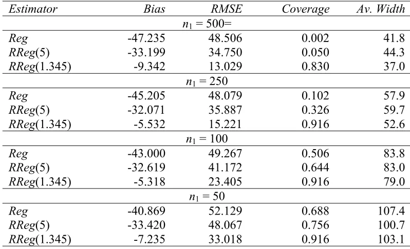
Examination of Tables 3 and 4 shows that even with a sample size as large as 500 and a sampling fraction of 0.5 the regression estimator generates PIs with below nominal coverage under MAR. Under NotMAR the bias in this estimator makes its PIs useless. In contrast, the robust regression estimator with c = 1.345 is extremely stable, but with a bias under MAR that makes its bootstrap-generated PIs increasingly useless as the sample size increases. Rather fortunately, this bias essentially cancels out under NotMAR, making its bootstrap PI coverage look much better. However, this is an artefact of the simulation method rather than any intrinsic property of these PIs. Finally, we see that in terms of RMSE the robust regression estimator with c = 5 seems a reasonable compromise under both MAR and NotMAR. Unfortunately, its bootstrap PIs have poor coverage in both situations.

Is this lack of coverage due to sample imbalance? Royall and Cumberland (1985) observed that most methods of variance estimation do not work well in unbalanced samples. However, when we examine the conditional behaviour under MAR of both the regression estimator error and the estimated standard error derived from (3) as the difference between the “sample” (s1) and “non-sample” (s2) means of X increases we see no decreasing trend in coverage. What we do see, however, is clear negative association between this error and the estimated standard error. There are too many samples where the estimated standard error is low and the estimation error is large and positive, leading to a decrease in coverage relative to nominal levels. Furthermore, this negative association is even more pronounced for the robust regression estimators, being most marked for c = 1.345.

[image:9.595.97.496.113.357.2]

Table 3 MAR simulation results for regression estimators. Average value of sample mean y_s

is 704.9.

Estimator Bias RMSE Coverage Av. Width

n1 = 500

Reg 2.436 8.050 0.902 27.9

RReg(5) 8.116 10.227 0.850 29.0

RReg(1.345) 21.825 22.321 0.056 21.5

n1 = 250

Reg 2.673 11.471 0.906 41.8

RReg(5) 7.584 11.848 0.874 36.8

RReg(1.345) 22.922 23.820 0.220 24.4

n1 = 100

Reg 2.072 18.124 0.914 66.7

RReg(5) 5.792 15.973 0.896 54.9

RReg(1.345) 21.737 24.048 0.574 38.0

n1 = 50

Reg 1.377 27.015 0.886 90.2

RReg(5) 2.686 22.877 0.876 76.1

RReg(1.345) 18.513 25.029 0.696 58.3

Table 4 NotMAR simulation results for regression estimators. Average value of sample mean

y_s is 704.4.

Estimator Bias RMSE Coverage Av. Width

n1 = 500=

Reg -47.235 48.506 0.002 41.8

RReg(5) -33.199 34.750 0.050 44.3

RReg(1.345) -9.342 13.029 0.830 37.0

n1 = 250

Reg -45.205 48.079 0.102 57.9

RReg(5) -32.071 35.887 0.326 59.7

RReg(1.345) -5.532 15.221 0.916 52.6

n1 = 100

Reg -43.000 49.267 0.506 83.8

RReg(5) -32.619 41.172 0.644 83.0

RReg(1.345) -5.318 23.405 0.916 79.0

n1 = 50

Reg -40.869 52.129 0.688 107.4

RReg(5) -33.420 48.067 0.756 100.7

RReg(1.345) -7.235 33.018 0.916 103.1

3 An Alternative Approach to Prediction Intervals

There are two basic assumptions that underpin use of prediction intervals in model-based sample survey theory. The first is that the conditional mean of Y given X in non-sampled part (r) of the population is same as that in the sampled part (s), i.e.

[image:9.595.96.495.411.654.2]

The second is that the estimator gˆ_s(x) of g_s(x) is unbiased at every value of X = x in the population. Both assumptions need not hold. The first is usually justified on the basis that s and r are defined through some form of random sampling. However, even if this is true, the second assumption can still fail, and in unbalanced samples it may be extremely difficult to detect this failure. If either assumption is invalid, standard PIs will fail, with the problem getting worse as the sample size increases.

Our alternative approach tackles these potential misspecification issues directly when forming a PI. That is, rather than generating an interval estimate to have a nominal level of coverage, we generate one that corresponds to a bound on the potential difference between the predicted values (the regression imputed values in the pay rate example) of Y and the actual non-sampled values of this variable. That is, we specify bounds gˆLs(x)≤ gˆs(x)≤ gˆUs(x) and then define our interval as [ ˆy_L, ˆy_U], where

ˆ

y_L = N−1 y_i+ gˆ_Ls(x_k) k_∉s

∑

i_∈s

∑

(

)

ˆ

y_U = N−1 y_i+ gˆ_Us(x_k) k_∉s

∑

i_∈s

∑

(

)

In order to implement this idea we need a sensible way of specifying bounds for non-sample data given sample data. A straightforward way of doing this is via quantile regression (Koenker and Bassett, 1978), where, rather than modelling the expected value of the conditional distribution f(y|x) of Y given X, we model the percentiles of this conditional distribution. In the linear case this leads to a family of linear models indexed by the value of the corresponding percentile “coefficient”, q ∈ (0,1), where for each value of q, the corresponding model shows how the qth percentile (quantile) of f(y|x) varies with x. Thus, the q = 0.5 line shows how the “middle” (median) of f(y|x) changes with x, while the general q -quantile line separates the “top” 100(1 - q)% of f(y|x) from the “bottom” 100q% - i.e. it represents conditional behaviour that is better than the worst 100q % in the data and worse than the best 100(1 - q)% in the data. Note that homoskedastic data will lead to parallel quantile regression lines, while heteroskedastic data will cause these lines to “spread out”.

Standard quantile regression lines can be unstable and non-unique. Breckling and Chambers (1988) introduced a generalisation of quantile regression models that they call M-quantile regression models. These models extend the quantile regression concept to robust regression defined by influence functions and can be fitted easily using iterated weighted least squares, with positive residuals weighted by q and negative residuals weighted by 1 – q. For any value of q we can then use the sample data to calculate robust q-quantile coefficients a_rreg(q)

,b_rreg(q) of a

linear model for the qth M-quantile of the conditional distribution of Y given X. These M-quantile regression lines have the same interpretation as q-quantile regression lines but depend on specification of an influence function. For ease of exposition, and because it works well in practice, we assume from now on that this influence function is Huber-type with tuning constant c. By construction (see Appendix 1) these lines are monotone in q over the range of population X-values and span virtually the entire range of the conditional distribution of Y given X.

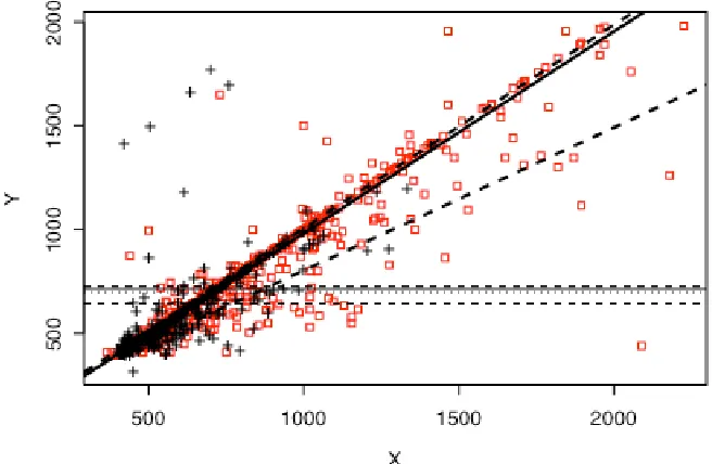
Let q < 0.5. The M-quantile interval (MQ-interval) for y_s corresponding to q is then

where yˆ_sq = N−1 y_i + (a_rreg(q) +b_rreg(q)x_i) s2

∑

s1

∑

[image:11.595.127.455.299.513.2]

(

)

. Note that the robust regression estimator is equal to yˆs0.5. Furthermore, the MQ-interval ( ˆysq, ˆys(1−q)) always includes this robust regression estimator, is generally not symmetric about yˆs0.5 and increases in width as q decreases to zero. Figure 2 illustrates the M-quantile regression fit to one sample from the MAR/n=500 simulation, and the resulting MQ-interval for the unknown value of y_s.

Figure 2 Scatterplot of data from one sample used in the MAR/n=500 simulation. The black “+” markers denote values from s1, while the red “” markers denote values from s2. The robust regression fit to the s1 data based on c = 1.345 is shown as a solid line while the corresponding M-quantile fits defined by q = 0.15 and q = 0.85 are shown as dashed lines. The horizontal lines show the estimated value of y_s based on this fit (solid line), the MQ-interval around this estimate corresponding to q = 0.15 (dashed lines) and the actual value of

y_s (dotted line).

It is important to realise from the outset that MQ-intervals are not confidence intervals and should not be interpreted as such. An MQ-interval represents an estimate of the range of possible values of y_s conditional on the regression M-median of the unobserved Y-values falling between the q and 1 – q regression M-quantiles of the observed Y-values. Our “confidence” in such an interval therefore depends on whether we believe this condition holds or not – it has nothing to do with the (repeated sampling) concept of coverage.

How then to choose q in (4)? Our preference is to adopt the same type of reasoning that is used to justify 95% as a “reasonable” nominal coverage level for general use in confidence intervals. In this case, a corresponding argument for q might be along the lines that it is extremely unlikely in practice that the non-sampled part of a population will have an average relationship between Y and X that is more extreme than that indicated by either the 25% or the 75% quantile regression lines in the sample. That is, we would choose q = .25 in (4) if the lines defined by the coefficients a_rreg(q) ,b_rreg(q) are quantile regression lines.

lines are closer together than corresponding quantile regression lines. It follows that we need to decrease q in this case. For the N(0,1) distribution the .25 quantile is -0.6745, while for the same distribution the .25 M-quantile with c = 1.345 is -0.4668. Equivalently, the .25 M-quantile defined by c = 1.345 is approximately the same as the .32 quantile of a N(0,1) distribution. Similarly, the .25 M-quantile corresponding to c = 5 approximately equates to the .33 quantile of a N(0,1) distribution. In fact, for c = 1.345, the .17 M-quantile is basically the same as the .25 quantile of a N(0,1) distribution, suggesting that if we want the interval defined by (4) to have the “level of protection” described in the previous paragraph, and our robust regression estimator is defined by c between 1.345 and 5, then a “safe” choice is to put q = .15 in (4).

An obvious problem with this argument is that ignores the impact of sample size and population variability on choice of q. Here, however, we can draw parallels with the coverage behaviour of confidence intervals. In particular, we suggest the following guidelines:

1. Given samples taken from a fixed population, as the sample size increases (decreases) the width of a prediction interval with a specified level of confidence decreases (increases). Consequently, under the same conditions, the value q should be chosen to increase towards (decrease away from) 0.5.

2. Given samples of the same size taken from populations with increasing (decreasing) variability, the width of a prediction interval with a specified level of confidence increases (decreases). Consequently, under the same conditions, the value q should be chosen to decrease away from (increase towards) 0.5.

Suppose now that we want to choose q so that the coverage probability of the associated MQ-interval is at least approximately known. Unfortunately, the preceding guidelines provide little help on what to do in this regard. What is needed is a more formulaic approach to choosing this parameter. We therefore again use normal theory to guide our choice and “map” an appropriate normal theory prediction interval with a specified level of coverage to an interval between the q and 1 - q quantiles of the underlying normal population distribution. The value q defined by this map is then used in (4).

How to choose an “appropriate” normal theory interval? Clearly there is nothing to be gained by taking the actual (and possibly flawed) interval generated by our estimation method (e.g. the robust regression estimator) and mapping this to a value of q since this will just recover the interval. Instead, we choose q so that it recovers the normal theory confidence interval in a situation where we believe the latter. In particular, let X_i;i∈s₁ ~ NID(µ,σ₁2) and

X_i;i∈s₂ ~ NID(µ,σ₂2). Furthermore, suppose we use the mean X₁ from s₁ to predict the overall mean X = N−1(nX₁+(N−n)X₂). Assuming uncorrelated population data, this mean has prediction variance

Var(X₁−X)= 1− n

N

⎛

⎝⎜ ⎞⎠⎟

2 σ1

2

n +

σ2 2

N −n

⎛ ⎝⎜

⎞ ⎠⎟.

X₁±2 1− n

N

⎛

⎝⎜ ⎞⎠⎟ σ1

2

n +

σ2 2

N−n .

In large samples this interval approximates the interval between the q and 1 - q quantiles of a

N(µ,σ₁2) distribution, where

q= Φ − 2 n 1−

n N

⎛

⎝⎜ ⎞⎠⎟ 1+

nσ₂2 (N−n)σ₁2

⎛ ⎝

⎜ ⎞

⎠ ⎟.

Given estimates σˆ₁ and σˆ₂(e.g. calculated via the procedure outlined in Appendix 2), we could therefore use the q-value

ˆ

qnorm = Φ − 2

n 1− n N

⎛

⎝⎜ ⎞⎠⎟ 1+

nσˆ₂2

(N −n) ˆσ₁2

⎛ ⎝

⎜ ⎞

⎠ ⎟

in (4). However, this interval is likely to be too small (i.e. q is too close to 0.5) because it assumes normal data, which is unlikely to be the case. We therefore put a non-conservative upper bound of 0.25 on q. Also, for values of q too close to zero (in particular, less than 1/n) the M-quantile fit becomes unstable, so we put a lower bound on q equal to the maximum of 1/n and 0.01. That is, our final expression for q in this case is

q=min(max(n−1, 0.01, ˆq_norm), 0.25). (5)

In order to evaluate the performance of MQ-intervals (4) defined either by a fixed “safe” choice of q (e.g. q = 0.15) or via a normal coverage map as specified by (5), we return to the NES simulation underlying Tables 3 and 4 and use the samples generated in this simulation to calculate MQ-intervals based on the robust regression estimators RReg(5.0) and RReg(1.345). The coverages and average widths of these intervals are displayed in Tables 5 to 8.

[image:14.595.96.496.96.299.2]

Table 5 Performance of fixed q MQ-intervals defined by robust estimates - MAR case

Coverage Average Width

q = 0.25 q = 0.15 q = 0.05 q = 0.25 q = 0.15 q = 0.05 n = 500

RReg(5) 1.000 1.000 1.000 50.0 82.6 168.1 RReg(1.345) 0.968 1.000 1.000 46.1 88.1 175.8

n = 250

RReg(5) 0.998 1.000 1.000 62.9 106.3 222.7 RReg(1.345) 0.932 0.998 1.000 57.1 110.2 227.7

n = 100

RReg(5) 0.954 0.996 1.000 72.1 125.5 256.4 RReg(1.345) 0.858 0.994 1.000 65.5 124.7 261.7

n = 50

[image:14.595.98.497.338.539.2]

RReg(5) 0.848 0.950 0.992 77.1 136.3 261.2 RReg(1.345) 0.776 0.946 0.994 72.7 132.7 282.3

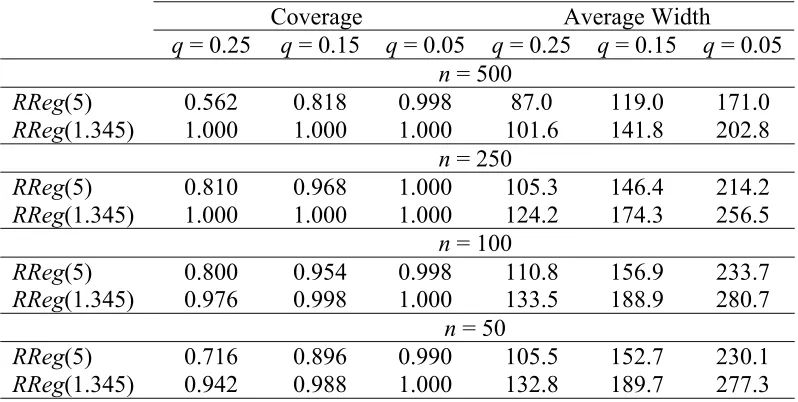
Table 6 Performance of fixed q MQ-intervals defined by robust estimates - NotMAR case

Coverage Average Width

q = 0.25 q = 0.15 q = 0.05 q = 0.25 q = 0.15 q = 0.05 n = 500

RReg(5) 0.562 0.818 0.998 87.0 119.0 171.0 RReg(1.345) 1.000 1.000 1.000 101.6 141.8 202.8

n = 250

RReg(5) 0.810 0.968 1.000 105.3 146.4 214.2 RReg(1.345) 1.000 1.000 1.000 124.2 174.3 256.5

n = 100

RReg(5) 0.800 0.954 0.998 110.8 156.9 233.7 RReg(1.345) 0.976 0.998 1.000 133.5 188.9 280.7

n = 50

RReg(5) 0.716 0.896 0.990 105.5 152.7 230.1 RReg(1.345) 0.942 0.988 1.000 132.8 189.7 277.3

Table 7 Performance of MQ-intervals where q is defined by (5) - MAR case.

Coverage (average q-value) Average Width n

RReg(5) RReg(1.345) RReg(5) RReg(1.345) 500 1.000

(0.250)

0.974 (0.214)

61.5 84.0

250 0.998 (0.249)

0.946 (0.218)

80.3 84.6

100 0.964 (0.240)

0.912 (0.191)

100.1 111.8

50 0.894

(0.228)

0.850 (0.170)

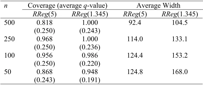
[image:14.595.126.467.580.721.2]

[image:15.595.126.466.97.240.2]

Table 8 Performance of MQ-intervals where q is defined by (5) - NotMAR case.

Coverage (average q-value) Average Width n

RReg(5) RReg(1.345) RReg(5) RReg(1.345) 500 0.818 (0.250) 1.000 (0.243) 92.4 104.5 250 0.968 (0.250) 1.000 (0.236) 114.0 133.1 100 0.956 (0.250) 0.986 (0.220) 124.4 153.2 50 0.868 (0.243) 0.948 (0.191) 124.8 168.0

4 An Application to Distribution Function Estimation

The gains from using MQ-intervals instead of confidence-based intervals become even more apparent when the target of inference is non-linear in Y. This is because variance estimation becomes more difficult in this case. To illustrate we consider the problem of estimating the distribution (rather than the mean) of hourly pay rates using the NES data. This estimated distribution is a key policy relevant output from the survey and is defined by

ˆ

F_s(t)= n−1 _s I(y_i ≤t)

1

∑

+ _s I(y_j ≤t)

2

∑

⎡

⎣ ⎤⎦

for t = 400, 425, …, 1000. As with estimation of the mean, we cannot calculate this statistic directly. Nor can we ignore the problem of the “missing” s2 data since the simple alternative distribution function estimate based just on the data in s1, i.e. Fˆs1(t)=n1

−1

I(y_i ≤t) s₁

∑

, is

highly biased (Skinner et al, 2003; Chambers, 2005). In contrast, a locally weighted predictor of Fˆ_s(t) based on the approach of Chambers and Dunstan (1986) works well. This is given by

ˆ

FCDL(t)= N

−1 _I(y

i≤t) i∈s₁

∑

+

wi(xj)I a

(

rreg+brregxj+ri ≤t

)

i∈s1

∑

wi(xj) i∈s1

∑

⎧ ⎨ ⎪ ⎩ ⎪ ⎫ ⎬ ⎪ ⎭ ⎪

j∈s₂

∑

⎛ ⎝ ⎜ ⎜ ⎜ ⎞ ⎠ ⎟ ⎟ ⎟ (6)

where r_i = y_i−a_rreg−b_rregx_i and w_i(x_j)=I x

(

_i −x_j ≤ f−1range(x)

)

is a “local” weight. The parameter f in this weight is chosen via a weighted type of cross-validation, with more importance attached to smaller values of t, see Chambers (2005) where the same MAR/n=500 and NotMAR/n =500 simulation data and samples as used previously are used to explore the performance of (6). Coverage results from two prediction interval methods based on (6) are presented below. For computational feasibility both require that the non-sample component of (6) be replaced by a weighted approximation, and are defined by:

(2) The 95% PI generated by applying a Naïve Bootstrap to FˆCDL(t). We denote this method by BOOT. Bootstrap World intervals were also investigated but provided poorer coverage.

Both methods gave very low coverage at all values of t when used with the MAR/n=500 simulation data (see Figure 4), so alternative MQ-intervals for Fˆ_s(t) based on (6) at each value of t were constructed. These intervals were defined by ( ˆFCDL

(q)

(t), ˆFCDL

(1−q)

(t)), where

ˆ

FCDL

(q)

(t)=N−1 I(yi ≤t) i∈s1

∑

+

wi(xj)I arreg

(q) _+b

rreg

(q)_x

j+ri

(0.5 ) _≤t

(

)

i∈s1

∑

wi(xj) i∈s1

∑

⎧ ⎨ ⎪ ⎩ ⎪ ⎫ ⎬ ⎪ ⎭ ⎪

j∈s2

∑

⎛ ⎝ ⎜ ⎜ ⎜ ⎞ ⎠ ⎟ ⎟ ⎟ .

Here a_rreg(q)

and b_rreg(q)

are the coefficients of the robust M-quantile fit to the s1 data at quantile coefficient q and ri

(0.5 ) ₌

yi−arreg

(0.5 )₋

brreg

(0.5 )

[image:16.595.108.423.199.252.2]

xi are the residuals from the median (q = 0.5) fit that defines (6).

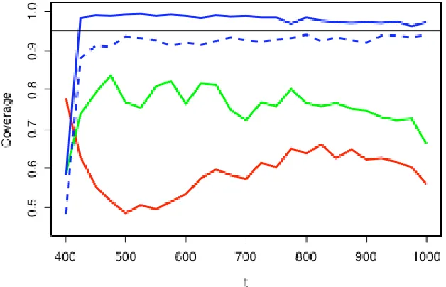
[image:16.595.127.456.483.700.2]

Figure 3 shows the q = 0.15 and q = 0.05 MQ-bounds for Fˆs(t) using the same sample as displayed in Figure 2. Figure 4 is a plot of the coverages of the LARGE, BOOT and two MQ-intervals defined by c = 1.345 (q = 0.15 and q defined by (5)) for the MAR/n=500 simulation. The superiority of the MQ-intervals is clear.

[image:17.595.124.438.146.348.2]

Figure 4 Coverage performance of prediction intervals for Fˆs(t) under MAR/n=500. Red line is LARGE method, green line is BOOT method and blue lines are M-quantile methods defined by c = 1.345 (solid line is fixed q = 0.15, dashed line is q defined by (5)).

5 Conclusions and Open Problems

In this paper we propose an alternative approach to the construction of prediction intervals in finite population estimation. These intervals are based on application of quantile regression ideas to estimation and are typically much simpler to compute than standard “confidence-based” prediction intervals when estimators are non-linear since they do not require estimation of the prediction variance of the estimator. Our empirical investigations also show that these MQ-intervals provide better coverage performance than standard methods in situations where the sample is highly unbalanced.

In developing MQ-intervals, however, we have implicitly assumed that, conditional on auxiliary information, population data are uncorrelated. In many situations this is unlikely to be the case, particularly where this auxiliary information is limited. Obvious examples are social surveys where little is known about the individuals making up the population beyond their locations. Here prediction methods typically allow for clustering in sample responses by assuming models with random cluster effects. The extension of the quantile modelling idea to this case needs to be investigated. Recent work on small area estimation based on M-quantile regression models (Chambers and Tzavidis, 2005) is an example of how this might work.

The most pressing area for further research, however, concerns specification of the “right” value of q to use when constructing an M-quantile interval. In this paper we make two pragmatic suggestions, both based on normal theory arguments. These worked well in our simulations, but a more rigorous approach to choice of this value is needed. Confidence intervals have the advantage that in large samples the central limit theorem allows specification of (nominal) coverage to be separated from specification of sample size and population variability. This separation does not exist for q. It is true that as population variability increases, quantiles generally “spread out” and so quantile-based intervals become wider. Consequently a fixed q MQ-interval will adapt to changes in population variability, provided these are reflected in changes in population quantiles. However, there is no natural mechanism for it to adapt to changes in sample size. In fact, since M-quantile regression has the same asymptotic behaviour as standard robust regression (Breckling and Chambers, 1988), these lines will, under the usual conditions, converge to the underlying population M-quantile lines, so their asymptotic coverage probability for fixed q < 0.5 is one. This may or may not be regarded as a good thing. What it does mean is that as n increases MQ-intervals will be wider than confidence intervals.

References

Breckling, J. and Chambers, R. (1988). M-quantiles. Biometrika75, 761-771.

Breidt, F.J. and Opsomer, J.D. (2000). Local polynomial regression estimators in survey sampling. Annals of Statistics28, 1026-1053.

Chambers, R.L. and Dunstan, R. (1986). Estimating distribution functions from survey data. Biometrika73, 597-604.

Chambers, R.L., Dorfman, A.H. and Wehrly, T.E. (1993). Bias robust estimation in finite populations using nonparametric calibration. Journal of the American Statistical Association 88, 268-277.

Chambers, R.L. (1996). Robust case-weighting for multipurpose establishment surveys. Journal of Official Statistics12, 3 - 32.

Chambers, R.L. and Dorfman, A.H. (2003). Robust sample survey inference via bootstrapping and bias correction: The case of the ratio estimator. Working Paper M03/13, Southampton Statistical Sciences Research Institute.

URL: http://www.s3ri.soton.ac.uk/publications/methodology.php

Chambers, R.L. (2005). Imputation vs. estimation of finite population distributions. Working Paper M05/06, Southampton Statistical Sciences Research Institute.

Chambers, R.L. and Tzavidis, N. (2005). M-quantile models for small area estimation. Working Paper M05/07, Southampton Statistical Sciences Research Institute.

Dorfman, A.H. (1992). Nonparametric regression for estimating totals in finite populations. Proceedings of the Section on Survey Research Methods, American Statistical Association, 622-625.

Koenker, R. and Bassett, G. (1978). Regression quantiles. Econometrica46, 33-50.

Presnell, P. and Booth, J.G. (1994). Resampling methods for sample surveys. Technical Report 470, Department of Statistics, University of Florida.

R Development Core Team (2004). R: A language and environment for statistical computing. R Foundation for Statistical Computing, Vienna, Austria. ISBN 3-900051-00-3, URL: http://www.R-project.org.

Royall, R.M. and Cumberland, W.G. (1981). The finite population linear regression estimator and estimators of its variance – An empirical study. Journal of the American Statistical Association76, 924-930.

Royall, R.M. and Cumberland, W.G. (1985). Conditional coverage properties of finite population confidence intervals. Journal of the American Statistical Association80, 355-359.

Skinner, C., Stuttard, N., Beissel-Durrant, G. and Jenkins, J. (2003). The measurement of low pay in the UK Labour Force Survey. Oxford Bulletin of Economics and Statistics64, 653-676.

Appendix 1 Calculation of monotone M-quantile regression lines

Given a sample of n values of Y and X drawn from some joint distribution, the coefficients

a_rreg(q) ,b_rreg(q)

of a linear model for the qth M-quantile of the corresponding conditional distribution of Y given X are obtained by using iteratively weighted least squares to solve the normal equations

φq(yk−arreg

(q) ₋

b_rreg(q)x_k) 1

x_k

⎛ ⎝⎜

⎞ ⎠⎟

k=1

n

∑

= 0

0

⎛ ⎝⎜

⎞

⎠⎟ (A1)

where φq(t)=qψ(s

−1

t)I(t >0)+(1−q)ψ(s−1

t)I(t ≤0) and s is a robust estimate of the scale of the residuals. In this paper we always define ψ as the Huber Proposal 2 influence function.

Typically, M-quantile lines defined by (A1) are fitted to a grid (qk) of quantile coefficients

spanning (0,1). However, there is no guarantee that these lines are monotone. That is, for

q_k <q_j on this grid, there is no guarantee that (a_rreg(qk)+_b

rreg

(q_k)

x)<(a_rreg(qj) +_b

rreg

(q_j)

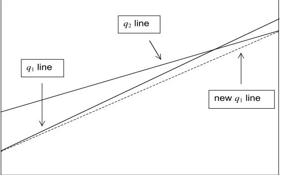
[image:20.595.162.447.552.729.2]

x) over any particular range of X values of interest. We therefore impose monotonicity ex-post relative to the fit at q = 0.5. That is, after estimating the coefficients a_rreg(q) ,b_rreg(q) on this grid, we sequentially “nudge down” lines corresponding to decreasing values of q < 0.5 and “nudge up” lines corresponding to increasing values of q > 0.5 in order to ensure that the final M-quantile lines defined by the grid are monotone over the range (x_min, x_max) of X-values of interest. This is done in a quite straightforward way by changing either the starting point or ending point of the line defined by the smaller (larger) value of q so that it is smaller (larger) than the corresponding point of the line defined by the larger (smaller) value of q. Figure 4 illustrates this procedure. Note that a consequence of this procedure is that the intercept and slope of any individual M-quantile line within the grid depends on the set of q-values that make up the grid. We use a default grid defined by q = 0.05, 0.1, 0.15, 0.2, 0.25,0.75, 0.8, 0.85, 0.9, 0.95.

Figure 4 Modification to M-quantile lines defined by q1 < q2 ≤ 0.5 to ensure monotonicity. Here q1 line crosses q2 line in the range of X-values of interest.

q1 line

q2 line

Appendix 2 Estimating σ₁ and σ₂

Estimates of σ₁ and σ₂ are needed to compute the normal theory-based q value (5). In order to obtain these estimates we fitted a weighted linear model to the logarithms of estimates of scale for groups within s1 and extrapolated this to provide an estimate of σ2. The steps in the procedure are set out below.

1. The range of X values across the entire sample is split into g equal width groups. 2. A zero-centred MAD estimate of scale is calculated for each group using the residuals

from the robust regression fit of Y on X corresponding to the s1 units in each group. 3. Logarithms of these group-level scale estimates are regressed against the average

values of X for the groups, using weights equal to the s2 count in each group. This fit is used to compute scale values for all groups.