Automatic Derivation of Statistical Data Analysis Algorithms: Planetary Nebulae and Beyond

Automatic Derivation of Statistical Data Analysis

Algorithms: Planetary Nebulae and Beyond

Bernd Fischer

, Arsen Hajian

_{, Kevin Knuth}

_{and Johann Schumann}

∗_{RIACS / NASA Ames Research Center}

†_{United States Naval Observatory}

∗∗_{NASA Ames Research Center}

Abstract. AUTOBAYESis a fully automatic program synthesis system for the data analysis domain. Its input is a declarative problem description in form of a statistical model; its output is documented and optimized C/C++ code. The synthesis process relies on the combination of three key techniques.

Bayesian networks are used as a compact internal representation mechanism which enables problem

decompositions and guides the algorithm derivation. Program schemas are used as independently composable building blocks for the algorithm construction; they can encapsulate advanced algo-rithms and data structures. A symbolic-algebraic system is used to find closed-form solutions for problems and emerging subproblems.

In this paper, we describe the application of AUTOBAYESto the analysis of planetary nebulae images taken by the Hubble Space Telescope. We explain the system architecture, and present in detail the automatic derivation of the scientists’ original analysis [1] as well as a refined analysis using clustering models. This study demonstrates that AUTOBAYESis now mature enough so that it can be applied to realistic scientific data analysis tasks.

INTRODUCTION

Planetary nebulae are remnants of dying stars. Scientists try to understand their physics by collecting and analyzing data, for example images taken by the Hubble Space Tele-scope (HST). The analysis follows a general pattern in science: formulate an initial un-derstanding of the underlying physical processes, formalize it as a statistical model, fit the model to the collected data, interpret the results, and refine the model as long as necessary. However, the large data volumes collected by modern instruments make computer support indispensable. Consequently, development and refinement of the nec-essary data analysis programs have become a bottleneck, and tapes of unanalyzed data often sit in warehouses, waiting for the software to be completed.

AUTOBAYES [2, 3] is a fully automatic program synthesis system for data

analy-sis problems which increases the speed with which reliable data analyanaly-sis software can be developed and thus eliminates this bottleneck. Its input is a declarative problem de-scription in form of a statistical model; its output is documented and optimized C/C++ code. Externally, it thus looks like a compiler; internally, however, it is quite different. AUTOBAYES first derives a customized algorithm implementing the model and then transforms it into code implementing the algorithm. The algorithm derivation or

synthe-sis process—which distinguishes AUTOBAYES from traditional compilers—relies on

(BNs) [4, 5] as a compact internal representation of the statistical models. BNs provide an efficient encoding of the joint probability distribution over all variables and thus en-able replacing expensive probabilistic reasoning by faster graphical reasoning. In partic-ular, they speed up the decomposition of a problem into statistically independent simpler subproblems. (ii) AUTOBAYESuses program schemas as the basic building blocks for the algorithm derivation. Schemas consist of a parameterized code fragment (i.e., tem-plate) and a set of constraints which are formulated as conditions on BNs. The templates can encapsulate advanced algorithms and data structures, which lifts the abstraction level of the algorithm derivation. The constraints allow the network structure to guide the ap-plication of the schemas, which prevents a combinatorial explosion of the search space. (iii) AUTOBAYEScontains a specialized symbolic-algebraic subsystem which allows it to find closed-form solutions for many problems and emerging subproblems. The com-bination of these techniques results in fast turnaround times comparable to compilation times, supporting the iterative development style typical for the domain. AUTOBAYES

thus enables the scientists to think and to program in models instead of code.

In this paper, we take one typical scientific data analysis problem—the analysis of planetary nebulae images taken by the HST—and show that AUTOBAYEScan be used to automate the implementation of the necessary programs. We initially follow the analysis by Knuth and Hajian [1] and use AUTOBAYESto derive code for the published models.

We show how concisely these models can be specified and how the code is derived; in particular, we show how the interaction between graphical reasoning, code instantiation, and symbolic computation is crucial for a fully automatic code derivation. We then go beyond the original analysis and use AUTOBAYES to derive code for a simple mixture model which can be used as an image segmentation procedure, automating a previously manual preprocessing step. Finally, we show how AUTOBAYESderives customized code

for modifications of the standard model, which yield a more detailed analysis. The main contribution of this paper is to demonstrate that AUTOBAYES has reached a level of maturity which makes it applicable to realistic scientific data analysis applications.

AUTOBAYES

AUTOBAYESis implemented in SWI-Prolog [6] and currently comprises about 75,000

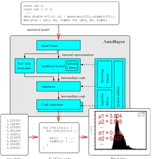
lines of documented code. Figure 1 shows the system architecture; in the following paragraphs we explain the major components.

3.232323 0 10 20 30 40 50 60 70 80 90 100

0.0 2.0 3.0 4.0 5.0 6.0 7.0 8.0 9.0

rel. class density

data class 1 class 2 class 3

...

σ2 = 0.437 σ1 = 0.103

...

µ2 = 2.948 µ1 = 3.024

C / C++ code

statistical model

Test−data

Generator Synthesis Kernel

Equation Solver Engine Rewriting intermediate code Optimizer AutoBayes Input Parser Code Generator } }

for i=0;i<n;i++ { for j=0;j<c;j++ {

mu[j] = ... sigma[j] = ... 3.342387 5.125683 3.891308 3.550812 5.412458 3.000217 2.994381 3.244621 ... const nat n. const nat c := 3.

data double x(I:=1..n) ~ gauss(mu(c(I)),sigma(c(I))). max pr(x | {phi, mu, sigma} for {phi, mu, sigma}.

raw data fitted data

Schema Library

System utilities

intermediate code internal representation

FIGURE 1. AUTOBAYESsystem architecture.

into the generated code to improve its legibility. Line 16 declares the observation (de-noted by the data-modifier) as a matrix; its expected properties are specified in the distribution clause in line 17. Distributions can be both discrete (e.g., binomial) or con-tinuous (e.g., Gaussian, Poisson, . . . ) but have to be univariate; support for multivariate distributions is currently under development. Distributions are chosen from a predefined list; adding more distributions is straightforward and requires only the definitions of the density functions. The final line in the model is the task clause. It specifies the anal-ysis problem the synthesized program has to solve. Since AUTOBAYES only supports

parameter learning (i.e., the estimation of the parameter values best explaining the

ob-served data, given a model) but not structure learning (i.e., the estimation of the best model itself), tasks have the form to maximize a conditional probability w.r.t. a set of goal variables. In this case, the task is a maximum likelihood estimation because all goal variables occur to the right of the conditioning bar in the conditional probability and there are no priors on the parameters. However, AUTOBAYEScan also solve maximum

a posteriori estimation (MAP) problems.

1 model gauss as ’2D Gauss-Model for Nebulae Analysis’.

% Image size

2 const nat nx as ’number of pixels, x-dimension’.

3 where 0 < nx.

4 const nat ny as ’number of pixels, y-dimension’.

5 where 0 < ny.

% Center; assume center is on the image

6 double x0 as ’center position, x-dimension’.

7 where 1 =< x0 && x0 =< nx.

8 double y0 as ’center position, y-dimension’.

9 where 1 =< y0 && y0 =< ny.

% Extent; assume full nebula is on the image

10 double r as ’radius of the nebula’.

11 where 0 < r && r < nx/2 && r < ny/2.

% Intensity; upper bound determined by instrument

12 double i0 as ’overall intensity of the nebula’.

13 where 0 < i0 && i0 =< 255.

% Noise; upper bound arbitrary, for initialization

14 double sigma as ’noise’.

15 where 0 < sigma && sigma < 100000.

% Data and Distribution

16 data double pixel(1..nx, 1..ny) as ’image’.

17 pixel(I,J) ~ gauss(i0*exp(-((I-x0)**2+(J-y0)**2)/(2*r**2)),

sigma).

% Task

18 max pr(pixel|{i0,x0,y0,r,sigma}) for {i0,x0,y0,r,sigma}.

FIGURE 2. Complete AUTOBAYES-specification for Gaussian model. Keywords have been underlined and line numbers have been added for reference; comments start with a % and extend to the end of the line.

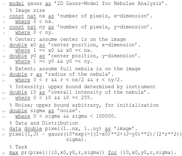
as continuous random variables; these are rendered as boxes and ellipses, respectively. However, in Figure 3 all variables are continuous. Shaded nodes represent known vari-ables, i.e., input data. Shaded boxes enclosing a set of nodes represent plates [4], i.e., collections of independent, co-indexed random variables. Distribution information for the random variables is attached to the respective nodes. Here, pixel is a nx×ny

ma-trix of independent and identically distributed (i.i.d.) Gaussian random variables with observed values.

Bayesian networks combine probability theory and graph theory. They are a common representation method in machine learning because they provide an efficient encoding of the joint probability distribution over all variables and thus allow to replace expensive probabilistic reasoning by faster graphical reasoning [4, 5].

Schemas and Schema Library. Program synthesis from first principles is notoriously difficult to scale up (cf. [8, 9]). AUTOBAYES thus follows a schema-based approach. A schema consists of a parameterized code fragment (i.e., template) and a set of con-straints. The parameters are instantiated by AUTOBAYES, either directly or by calling

FIGURE 3. Bayesian net for Gaussian model, automatically extracted from the Gaussian model speci-fication and drawn using thedotgraph layouting package [7].

the task clause as special case. This allows the network structure to guide the applica-tion of the schemas and thus to constrain combinatorial explosion of the search space, even if a large number of schemas is available. Schemas are implemented as Prolog-clauses and search control is thus simply relegated to the Prolog-interpreter: schemas are tried in their textual order. This simple approach has not caused problems so far, mainly because the domain admits a natural layering which can be used to organize the schema library. The top layer comprises network decomposition schemas which try to break down the network into independent subnets, based on independence the-orems for Bayesian networks. These are domain-specific divide-and-conquer schemas: the emerging subnets are fed back into the synthesis process and the resulting programs are composed to achieve a program for the original problem. AUTOBAYESis thus able to automatically synthesize larger programs by composition of different schemas. The next layer comprises more localized decomposition schemas which work on products of

i.i.d. variables. Their application is also guided by the network structure but they require

more substantial symbolic computations. The core layer of the library contains statistical algorithm schemas as for example expectation maximization (EM) [10, 11] and k-Means (i.e., nearest neighbor clustering); these generate the skeleton of the program. The final layer contains standard numeric optimization methods as for example the Nelder-Mead simplex method or different conjugate gradient methods. These are applied after the sta-tistical problem has been transformed into an ordinary numeric optimization problem and if AUTOBAYES failed to find a symbolic solution for the problem. Currently, the

library consists of 28 top-level schemas, with a number of additional variations (e.g., different initializations).

Symbolic Subsystem. AUTOBAYESrelies significantly on symbolic computations to

support schema instantiation and code optimization. The core part of the symbolic sub-system implements symbolic-algebraic computations, similar to those in Mathematica [12]. It is based on the concept of term rewriting [13] and uses a small but reason-ably efficient rewrite engine. Expression simplification and symbolic differentiation are implemented as sets of rewrite rules for this rewrite engine. The basic rules are straight-forward; however, the presence of vectors and matrices introduce a few complications and require a careful formalization. In addition, AUTOBAYEScontains a rewrite system

which implements a domain-specific refinement of the standard sign abstraction where numbers are not only abstracted into pos and neg but also into small (i.e., |x|<1) and

large. AUTOBAYESthen uses a relatively simple symbolic equation solver built on top

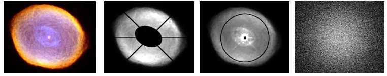
FIGURE 4. Planetary nebula IC 418 or Spirograph Nebula (a) Composite false-color image taken by the HST (Sahai et al., NASA and The Hubble Heritage Team). The different colors (resp. gray-scales) indicate the different chemicals prevalent in the different regions of the nebula; the origin of the visible texture is still unknown. The central white dwarf is discernible as a white dot in the center of the nebula. (b) Manually masked original image. (c) Original image with estimated Gaussian model parameters superimposed. (d) Sample data generated using estimated Gaussian model parameters.

roots and bi-quadratic forms, and tries to find polynomial factors, and handles expres-sions in x and(1−x)which are common in statistical applications.

A smaller part of the symbolic subsystem implements the graphical reasoning rou-tines necessary for Bayesian networks with plates, for example, computing the parents, children, or Markov blanket [5] of a node.

Backend. The code constructed by schema instantiation and composition is repre-sented in an imperative intermediate language. This is essentially a “sanitized” subset of C (e.g., no pointers), which is extended by a number of domain-specific constructs like vector/matrix operations, finite sums, and convergence-loops. Since straightforward schema application can produce suboptimal code, AUTOBAYES interleaves synthesis

and code optimization (cf. [14] for an overview of advanced optimization techniques). Schemas can explicitly trigger aggressive large-scale optimizations like code motion, common sub-expression elimination, and memoization which can take advantage of in-formation from the synthesis process. Traditional low-level optimizations like constant propagation or loop fusion, however, are left to the compiler. In a final step, AUTOBAYES

translates the intermediate code into code tailored for a specific run-time environment. Currently, AUTOBAYES includes code generators for the Octave and Matlab environ-ments; it can also produce stand-alone C and Modula-2 code. Each code generator is implemented as a rewrite system which eliminates the intermediate language constructs not supported by the target environment; most rules are shared between the different code generators.

Test-Data Generation. Statistical models also allow to generate problem-specific test data (i.e., sampling), if the the edges of the extracted network are followed forward from the sources and random numbers are generated along the way. AUTOBAYESuses this interpretation to generate model-specific sampling programs which can be used to validate the models and solutions.

PLANETARY NEBULAE

fusion, resulting in a carbon-oxygen core roughly the size of the earth. Eventually, the secondary fusion runs out of fuel as well and the red giants begin to collapse into ex-tremely hot white dwarfs. During this collapse, most of the material is expelled, forming blown-out gaseous shells which are called planetary nebulae. The shells continue to ex-pand and after 10,000 to 50,000 years their density becomes too small for the nebulae to be visible. Figure 4(a) shows an image of the planetary nebula IC 418.

Planetary nebulae occupy an important position in the stellar life cycle and are the major sources of interstellar carbon and oxygen but their physics and dynamics are not yet well understood. The characterization and analysis of their properties is thus an important task in astronomy.

A HIERARCHICAL SET OF MODELS

Knuth and Hajian [1] present a hierarchical set of three models they use to analyze im-ages of the planetary nebula IC418 (cf. Figure 4(a)). Each model estimates a parameter set which is then refined by the subsequent models. Their common idea is (i) that the light intensity which is expected at a given pixel position(x,y)on the image can be de-scribed by a function F of this position, the (unknown) nebula center(x₀,y₀), and some additional parameters, and (ii) that the measured intensities can be fitted against F us-ing a maximum likelihood estimation of the parameters, which results in a simple mean square error minimization due to the Gaussian likelihood. The only difference between the models is the form of F.

Here we sketch how these models are represented in AUTOBAYES’ specification

language, and how the code is derived. In particular, we show how the interaction between graphical reasoning, code instantiation, and symbolic computation is crucial for a fully automatic code derivation.

Gaussian Model

The most simple model describes the nebula as a blurred two-dimensional Gaussian cloud. The function F thus describes the shape of a bell whose apex is at(x₀,y₀)which can be formalized by a two-dimensional Gaussian curve:

F(x,y) =i₀·e−

(x₀−x)2_+(y 0−y)2

2r2 ₍₁₎

The additional parameters i₀and r capture the overall intensity and extent of the nebula (i.e., the height and diameter of the bell).

Model Specification. The AUTOBAYES specification shown in Figure 2 is a direct

additional assumptions on the structure of the image or the output of the instrument (cf. line 13).

Mathematical Derivation. For the Gaussian model, the program derivation can neatly be separated into two phases such that the first phase is a purely mathematical derivation and the second phase only instantiates code templates. In general, however, this is not the case and symbolic computation and template instantiation are interleaved. The first step is to unfold the entire pixel-matrix element by element, using a decom-position schema based on the conditionalized version of the general product rule for probabilities:

pr(pixel|i₀,x₀,y₀,r,σ) =∏nxi=1∏ ny

j=1pr(pixel(i,j)|i0,x0,y0,r,σ)

The precondition for this step is that the pixels are pairwise independent, given the remaining variables, i.e., that

pr(pixel(i,j)|pixel(i0,j0),i₀,x₀,y₀,r,σ) =pr(pixel(i,j)|i₀,x₀,y₀,r,σ)

holds for all i,j,i0,j0 such that i6=i0 or j6= j0. Instead of proving this from first princi-ples, using the distribution information given in the model specification, AUTOBAYES

can easily check it on the Bayesian network: there is no edge going from the pixel-node into itself and, hence, by definition of Bayesian networks, the pixels are pairwise inde-pendent.

The probability is now elementary in the sense that on the left of the conditioning bar we have only a single variable pixel(i,j)which depends exactly on all the variables to the right of the conditioning bar. Hence, the probability expression can be replaced by the distribution function. AUTOBAYES’s domain theory contains rewrite rules for the most common probability density functions; additional density functions can easily be added. This rewrite yields the likelihood-function

∏nx

i=1∏ ny

j=1

1 √

2π σ2

·e−



pixel(i,j)−i0·e

−(x0−i)2+(y0−j)2 2r2





2

2σ2

which must be maximized w.r.t. goal variables io, x₀, y₀, r, and σ. In general it is

easier to work with the log-likelihood function which yields the same solutions during maximization since the logarithm is strictly monotone. After simplification using the symbolic subsystem, AUTOBAYESthus derives the following log-likelihood function:

L=−nx·ny·log(2π)−nx·ny·log(σ)− 1

2σ2·∑

nx i=1∑

ny j=1

pixel(i,j)−i₀·e−

(i−x₀)2_+(j−y 0)

2

2r2

2

A solution can now be attempted in two different ways, numerically or symbolically. By default, AUTOBAYEStries to find symbolic solutions first. In this case, it computes the partial differentials

∂L

∂i₀ =

1

σ2·∑

nx i=1∑

ny

j=1pixel(i,j)·e

−(i−x0)2+(j−y0)2)

2r2 ₋ i0

σ2·∑

nx i=1∑

ny j=1e

−(i−x0)2+(j−y0)2)

r2

∂L

∂ σ =

1

σ3·∑

nx i=1∑nyj=1

pixel(i,j)−i₀·e−

(i−x0)2+(j−y0)2)

2r2

2

and solves the equations ∂L/∂i₀ =! 0 and ∂L/∂ σ =! 0 which are essentially simple

polynomials in i₀ and σ. These can easily be handled by the built-in equation solver;

however, attempts to solve for the remaining three variables x₀, yo, and r fail.

Code Derivation. At this point, the symbolic computations have been exhausted with-out leading to a complete symbolic (i.e., closed-form) solution. AUTOBAYESthus

de-rives code for a numeric solution, incorporating the computed partial symbolic solution. This is done in two steps, which correspond to schemas in the schema library.

In the first step, AUTOBAYESconverts the symbolic solutions into assignment

state-ments. Then it identifies their order and position relative to the remaining code which is still to be synthesized. Since both solutions contain at least one (in fact all) of the remaining variables, they must follow that code. Similarly, since the solution forσ

con-tains i₀, its assignment must in turn follow that of i₀. AUTOBAYESthen eliminates both variables from the formula by applying the substitution corresponding to the solution. Variables whose solutions do not depend on any unsolved variable can be considered as symbolic constants and need not be eliminated; their corresponding assignments must precede the missing code block. Since this reasoning is done on the expression level, and expression evaluation is free of side-effects, a dataflow analysis is not required.

In the second step, AUTOBAYES instantiates a numeric optimization routine, in this case the Fletcher-Reeves conjugate gradient method. The schema’s template actually contains a wrapper to the implementation provided by the GNU Scientific Library (GSL) [15]. However, the schema itself contains not just boilerplate code but also constructs specific initialization code and a number of auxiliary functions to evaluate the goal function and the derivatives. AUTOBAYES contains different heuristics to derive

ini-tialization code from specification information; here, the initial values are taken as the midpoints of the specified ranges. AUTOBAYESalso generates the auxiliary functions; since a straightforward translation from the goal expression would be prohibitively inef-ficient, AUTOBAYESaggressively optimizes the auxiliary functions. The optimizations applied here include common subexpression elimination, memoization (i.e., caching of expressions which depend on int-variables), and code motion. They are applied both intra- and inter-procedural, although the latter is restricted to the generated auxiliary functions. The optimizations can also take into account locally constant variables, since AUTOBAYESknows the set of goal variables. Again, a dataflow analysis is not required

since the reasoning is done on the expression-level.

Program Results. We have applied the generated program to the manually masked image of IC418 shown in the second panel of Figure 4. The third panel shows the results. The program roughly approximates the center but its estimate of the overall extent is predictably off the mark. The last panel shows sample data generated using the estimated Gaussian model parameters.

Sigmoidal Models

clearly elliptic, with a broad intensity plateau and a pronounced falloff at the edges. Simple Sigmoidal Model. Knuth and Hajian thus refine their initial model and re-place the two-dimensional Gaussian by a two-dimensional sigmoidal function of the form

F(x,y) =i₀·

"

1− 1

1+e−a

√ r(x,y)−1

#

(2)

with the auxiliary function r(x,y)

r(x,y) =cxx·(x₀−x)2+2cxy·(x₀−x)(y₀−y) +cyy·(y₀−y)2

and constants cxx, cyy, and cxy

cxx=cos 2

θ

rx2

+sin2θ

rx2

cyy=sin 2

θ

r2x

+cos2θ

r2x

cxy= sinθ·cosθ

r2x·r2y

where rx and ry are the extent of the nebula along the major and minor axis, resp.,θ is its orientation, and a the intensity falloff.

The specification for this modified model can easily be derived from the one for the Gaussian model shown in Figure 2, essentially by replacing the mean value in the distribution clause (cf. line 17) with the new version of F and adding declarations for the new model variables. The auxiliary constants and functions are represented as deterministic nodes in the Bayesian network, which are expanded like C-style macro definitions during the program definition. The program for this model is then derived using the same steps as before; the only difference is that the symbolic expressions become much more complicated.

Axis-aligned Sigmoidal Model. The derivation and resulting program can be simpli-fied and sped up, if the nebula image is assumed to be axis-aligned. This can be modeled by changing the random variableθ into a constant with known value, i.e.,

const double theta := 0 as ’orientation’.

AUTOBAYEScan then propagate this constant value already on the specification level and derive code from the simplified model.

Dual Sigmoidal Model. In a final refinement step, Knuth and Hajian try to estimate the thickness of the shell as well. Since projecting the three-dimensional ellipsoidal shell of gas onto a two-dimensional image produces an ellipsoidal blob surrounded by a ring of higher intensity, the image can be modeled as the difference of two sigmoidal func-tions with the same center and orientation but different extents, intensities, and falloffs. Re-using the auxiliary definitions from the simple sigmoidal model, this refinement can also be specified easily for AUTOBAYES.

IMAGE SEGMENTATION MODELS

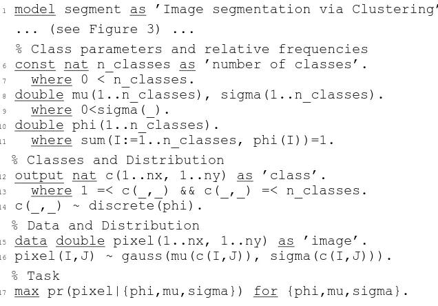
1 model segment as ’Image segmentation via Clustering’.

... (see Figure 3) ...

% Class parameters and relative frequencies

6 const nat n_classes as ’number of classes’.

7 where 0 < n_classes.

8 double mu(1..n_classes), sigma(1..n_classes).

9 where 0<sigma(_).

10 double phi(1..n_classes).

11 where sum(I:=1..n_classes, phi(I))=1.

% Classes and Distribution

12 output nat c(1..nx, 1..ny) as ’class’.

13 where 1 =< c(_,_) && c(_,_) =< n_classes.

14 c(_,_) ~ discrete(phi).

% Data and Distribution

15 data double pixel(1..nx, 1..ny) as ’image’.

16 pixel(I,J) ~ gauss(mu(c(I,J)), sigma(c(I,J))).

% Task

17 max pr(pixel|{phi,mu,sigma}) for {phi,mu,sigma}.

FIGURE 5. AUTOBAYES-specification for image segmentation model.

into different conceptual classes (e.g., central star, nebula, and background) can replace the generic mask. In this section we show how AUTOBAYEScan be used to derive code for this and further refined segmentation models.

Segmentation via Clustering. The simplest segmentation model is the straightfor-ward Gaussian mixture model shown Figure 5. At its core is the latent variable c (cf. lines 12–14) which represents the unknown class each pixel belongs to and which de-termines the mean and variance (cf. line 16); its values are independently drawn from a discrete distribution with relative frequenciesϕ, i.e., pr(c_{i j}=k) =ϕ_k. The constraint on

the probability vectorϕ (cf. line 11) is required to make this model well-formed. Since

we need the class-assignments for the segmentation, c is declared asoutput. Note that the model assumes that the number of classes is known.

AUTOBAYES solves this model by an application of the EM-schema which is trig-gered by the latent variable structure of the corresponding Bayesian network. After in-stantiation of the EM-schema, all emerging sub-problems (for the E- and M-step) can eventually be solved symbolically (for the detailed derivation cf. [2, 3]).

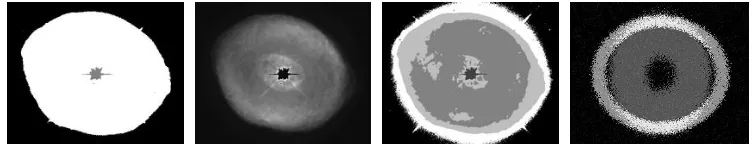
Figure 6 shows the result of segmenting the IC418 image according to the identified different classes. In particular, a segmentation into three classes already isolates the central star, the nebula, and the background from each other. It can thus be used as a precise, image-specific mask (cf. Figures 4(b) and 6(a)). More classes reveal more details, e.g., identify the nebula’s shell and separate the halo from the background, but too many classes bear the usual risk of overfitting the image.

Model modifications. Code implementing this standard model can be found in many libraries. AUTOBAYES, however, can also derive customized code for model

modifica-tions. For example, a uniform variance for all classes can be enforced by simply chang-ing the distribution clause into

FIGURE 6. Segmentations of IC418 image: (a) three-class segmentation (b) ditto, white class used as mask load to original image (c) five-class segmentation, and (d) sample data from geometrically refined segmentation model; class 1 (white) corresponds to the hull, class 2 (gray) to the core, and class 3 (not shown) to the background.

and adapting the declaration ofσ accordingly. AUTOBAYESstill solves this model by an

application of the EM-schema as before, but the structure of the M-step changes. In the standard model, it contains a loop over all classes which computes the current estimates ofµ_iandσ_i. In the modified model, only the µ_iare computed inside the loop, while the

singleσ is computed separately. This modification cannot be achieved by simple code

parametrization—it requires an actual code adaptation.

Similarly, the standard model can be refined by adding priors (e.g., on the class means) to capture additional background knowledge. In AUTOBAYES, these priors are simply

added to the specification as distribution clauses for the parameters. For example, a conjugate prior on each individual mean can be specified by

mu(I) ~ gauss(mu0(I), sqrt(sigma_sq(I)) * kappa0(I)).

AUTOBAYES again solves the model by an application of the EM-schema, and again the structure of the M-step changes, now to reflect the MAP estimate. More model modifications can be specified easily: a conjugate prior using the same parameters for all class means, non-conjugate priors, a mixture of different distributions (e.g., a single Cauchy and multiple Gaussians), and many more. In each case, AUTOBAYES derives an appropriate version of the EM-algorithm, instantiating and composing schemas as required. This makes it much more flexible than a simple code library.

Multivariate approximation. Images of planetary nebulae are taken at different wavelengths, usually in the infrared and visible bands. Such data sets can be analyzed by AUTOBAYESif the covariance matrix is (assumed to be) diagonal, even though AUTO -BAYEScannot yet properly handle multivariate distributions. In the specification shown in Figure 5, only the declaration (line 15) and distribution (line 16) of the input data need to be modified as shown below. Again, AUTOBAYES generates an appropriately

instantiated EM algorithm.

data double pixel(1..nc,1..nx, 1..ny) as ’data cube’. pixel(C,I,J) ~ gauss(mu(C,c(I,J)), sigma(C,c(I,J))).

around the center x₀(c_{i j}),y₀(c_{i j}) with radii rx(c_{i j}) and ry(c_{i j}), and a thickness d(c_{i j}). Each of these unknown parameters depend on the class c_{i j} of each pixel at position i,j.

In the AUTOBAYES specification of Fig 5, we only need to replace the simple mean

µ(c_{i j})of the Gaussian distribution (cf. line 16) by the expression

i₀(c_{i j})·e−

(√r(i,j)−1)2_·(r

x(ci j)2+ry(ci j)2)

4d(c_{i j})2

(3)

where r(i,j) = (i−rx(c_{i j}))2/rx(c_{i j})2+ (j−ry(c_{i j}))2/ry(c_{i j})2. AUTOBAYESagain syn-thesizes an EM-algorithm, this time with a numerical optimization routine (e.g., a Nelder-Mead simplex method) nested within the M-step. Figure 6(d) shows sampling data generated with the parameters estimated by this model.

EVALUATION

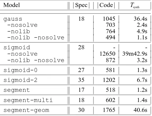
Table 1 summarizes the results; it shows that AUTOBAYES’s specification language allows a compact problem representation: none of the models discussed here required more than 35 lines of specification. The major difficulty in writing the specifications was to understand and then to express the core idea of the original models. After that, each specification took only a few minutes to write and in general one or two iterations to debug and complete (e.g., adding constraints).

The table also shows the overall feasibility of the approach. AUTOBAYESwas able to derive code for each of the models; scale-up factors from the model specification to the generated code are generally around 1:30. Synthesis times are generally only a few seconds and comparable to compilation times of the derived code. However, for the gauss and sigmoid models, AUTOBAYES spends almost all time simplifying

the partial differentials and then optimizing the auxiliary functions evaluating them; in the sigmoid-case, this even exhausts the available memory. With the command line options-nosolveand-nolib, AUTOBAYEScan be forced to stay away from these

expensive calculations and code is derived much faster, using the Nelder-Mead simplex method which requires no differentials.

Search space explosion is a common problem in program synthesis. In our case, it is mitigated by the deterministic nature of the symbolic-algebraic computations, the higher level of abstraction inherent to the schemas, and the inherent structure of the schema library. Still, search spaces are large since schemas can be functionally equivalent and solve the same class of problems. For the gauss-model, AUTOBAYES derives 224

programs, many of them identical, in 35 minutes total synthesis time. Parts of the search space can be pruned away manually by command line options like-nosolve, but more implicit control is required, especially when the schema library grows further.

The original Matlab code written by the Knuth [1] uses a gradient descent method; it computes the differentials in a single iteration over all pixels while the synthesized code iterates once for each differential but reuses memoized subexpressions. This de-composition requires domain knowledge not yet formalized for AUTOBAYES. For the

TABLE 1. Summary of Results. For each model, the size of the specification|Spec|and the generated program (including generated comments)|Code|, and the synthesis time Tsynth(measured on an unloaded

2GHz/4GB LinuxPC) are given. -nosolve and-nolib are AUTOBAYES command line options which suppress the application of the schemas using partial symbolic solutions and library components. The entries forsigmoid-0,sigmoid-2, andsegment-geomrefer to the -nolib -nosolve

variants.

Model |Spec| |Code| Tsynth

gauss 18 1045 36.4s

-nosolve 703 2.4s

-nolib 764 4.9s

-nolib -nosolve 494 1.1s

sigmoid 28 -

--nosolve 12650 39m42.9s

-nolib -nosolve 872 3.2s

sigmoid-0 27 581 1.3s

sigmoid-2 35 1202 6.7s

segment 17 518 1.2s

segment-multi 18 602 1.4s

segment-geom 30 1765 40.6s

for the computation of the gradient. It requires on average 174 seconds to converge, while the synthesized C++-code only requires 11 seconds.

RELATED WORK

Scientific computing is a (relatively) popular application domain for program synthesis; due to its complexity, most related work also follows a schema-based approach. How-ever, most work focuses on wrapping solvers for partial differential equations (PDEs). SciNapse [16] is a general “problem-solving environment” for PDEs; it supports code generation for a variety of features in the PDE-domain, as for example coordinate trans-formation or grid generation. Ellman et al. [17] describe a system to generate simulation programs from PDEs. Both systems use Mathematica as underlying symbolic engine. Ctadel [18] is PDE-based synthesis system for the weather forecasting domain. Like AUTOBAYES, it is implemented in SWI-Prolog and contains its own symbolic engine.

Other domains than PDEs have been tackled less often. Amphion [19] is a purely deductive synthesis system which has been used to synthesize astronomical software using library components. Amphion/NAV [20] applies the same technology to the state estimation domain. The scale-up difficulties encountered there led to a switch to a schema-based approach and the development of the AUTOFILTER-system [21] as a

structure the domain theory and thus to reduce the required proof effort.

Schema-based program synthesis is also related to generative programming [23], since schemas (more precisely, the code fragments) correspond to templates. The major differences are that (i) the almost completely syntax-directed template instantiation is less powerful and less secure than schema instantiation and (ii) the users still have to write the core algorithm.

Code libraries are common in scientific computing and data analysis, but they lack the level of automation achievable by program synthesis. For example, the Bayes Net Toolbox [24] is a Matlab library which allows program development on the model level, but it does not derive algorithms or generate code. BUGS [25] is a statistical model interpreter based on Gibbs-sampling, a more general but less efficient Bayesian inference technique; it could be integrated into AUTOBAYESas an additional schema.

CONCLUSIONS

We presented AUTOBAYES, a fully automatic program synthesis system for the data

analysis domain and demonstrated how it can be used to support a realistic scientific task, the analysis of planetary nebulae images taken by the HST. We specified the hierarchy of models presented in [1]. AUTOBAYESwas able to automatically generate code for these

models; in tests, the synthesized code gave the same results as the scientists’ Matlab code. We also used AUTOBAYESto refine the analysis, combining cluster-based image segmentation with geometric constraints.

Key elements to achieve these results are the schema-based synthesis approach, an ef-ficient problem representation via Bayesian networks, and a strong symbolic-algebraic subsystem. This combination is unique to AUTOBAYESand allows us to solve realistic

data analysis problems. In this particular case study the recently completed integration of the GSL and the aggressive optimization of the goal expressions proved to be instru-mental to derive efficient code.

However, AUTOBAYESmust still be improved before it can be delivered to the

work-ing data analyst. In particular, the domain coverage must be extended and schemas must be added to enable solutions for new classes of models (e.g., multivariate distributions). Synthesis from large models requires support for hierarchical specifications and more powerful optimizations to generate faster code. Finally, numeric optimization schemas must be extended with numeric constraint handling to produce more versatile and robust code. Yet, AUTOBAYES already demonstrates that program synthesis technology has

become a viable and versatile technology that enables scientists to think and to program in models rather than in code.

Availability. A web-based interface to AUTOBAYES and links to other papers are available at

http://ase.arc.nasa.gov/autobayes.

Acknowledgments. A. Hajian was supported for this work by NASA through grant numbers GO7501,

REFERENCES

1. Knuth, K. H., and Hajian, A. R., “Hierarchies of Models: Toward Understanding of Planetary Nebulae,” in Proc. Bayesian Inference and Maximum Entropy Methods in Science and Engineering, edited by C. Willimans, American Institute of Physics, 2002, pp. 92–103.

2. Fischer, B., and Schumann, J., J. Functional Programming, 13, 483–508 (2003).

3. Gray, A. G., Fischer, B., Schumann, J., and Buntine, W., “Automatic Derivation of Statistical Algo-rithms: The EM Family and Beyond,” in Advances in Neural Information Processing Systems 15, edited by S. Becker, S. Thrun, and K. Obermayer, MIT Press, 2003, pp. 689–696.

4. Buntine, W. L., J. AI Research, 2, 159–225 (1994).

5. Pearl, J., Probabilistic Reasoning in Intelligent Systems: Networks of Plausible Inference, Morgan Kaufmann Publishers, 1988.

6. Wielemaker, J., SWI-Prolog 5.2.9 Reference Manual, Amsterdam (2003).

7. Koutsofios, E., and North, S., Drawing graphs with dot, Tech. rep., AT&T Bell Laboratories, USA (1996).

8. Ayari, A., and Basin, D., J. Symbolic Computation, 31, 487–520 (2001).

9. Manna, Z., and Waldinger, R., The Deductive Foundations of Computer Programming, Addison-Wesley, 1993.

10. Dempster, A. P., Laird, N. M., and Rubin, D. B., J. of the Royal Statistical Society series B, 39, 1–38 (1977).

11. McLachlan, G., and Krishnan, T., The EM Algorithm and Extensions, Wiley Series in Probability and Statistics, John Wiley & Sons, New York, 1997.

12. Wolfram, S., The Mathematica Book, Cambridge Univ. Press, Cambridge, UK, 1999, 4th edn. 13. Baader, F., and Nipkow, T., Term Rewriting and all that, Cambridge Univ. Press, Cambridge, 1998. 14. Muchnick, S. S., Advanced Compiler Design and Implementation, Morgan Kaufmann Publishers,

San Mateo, CA, USA, 1997.

15. Galassi, M., Davies, J., Theiler, J., Gough, B., Jungman, G., Booth, M., and Rossi, F., GNU Scientific Library - Reference Manual (2002), edition 1.3, for GSL Version 1.3.

16. Akers, R., Baffes, P., Kant, E., Randall, C., Steinberg, S., and Young, R., IEEE Computational

Science and Engineering, 4, 33–42 (1997).

17. Ellman, T., Deak, R., and Fotinatos, J., “Knowledge-Based Synthesis of Numerical Programs for Simulation of Rigid-Body Systems in Physics-Based Animation,” in Proc. 17th Intl. Conf. Automated

Software Engineering, edited by W. Emmerich and D. Wile, IEEE Comp. Soc. Press, 2002, pp. 93–

104.

18. van Engelen, R. A., Wolters, L., and Cats, G., “Ctadel: A Generator of Efficient Code for PDE-based Scientific Applications,” in Proc. 9th Intl. Conf. on Supercomputing, ACM Press, 1996, pp. 86–93. 19. Stickel, M., Waldinger, R., Lowry, M., Pressburger, T., and Underwood, I., “Deductive Composition

of Astronomical Software from Subroutine Libraries,” in Proc. 12th Intl. Conf. Automated Deduction, edited by A. Bundy, Springer, 1994, vol. 814 of Lect. Notes Artificial Intelligence, pp. 341–355. 20. Whittle, J., Van Baalen, J., Schumann, J., Robinson, P., Pressburger, T., Penix, J., Oh, P., Lowry, M.,

and Brat, G., “Amphion/NAV: Deductive Synthesis of State Estimation Software,” in Proc. 16th Intl.

Conf. Automated Software Engineering, edited by M. S. Feather and M. Goedicke, IEEE Comp. Soc.

Press, 2001, pp. 395–399.

21. Whittle, J., and Schumann, J., Automating the Implementation of Kalman-Filter Algorithms (2003), in review.

22. Blaine, L., Gilham, L.-M., Liu, J., Smith, D. R., and Westfold, S., “Planware – Domain-Specific Syn-thesis of High-Performance Schedulers,” in Proc. 13th Intl. Conf. Automated Software Engineering, edited by D. F. Redmiles and B. Nuseibeh, IEEE Comp. Soc. Press, 1998, pp. 270–280.

23. Czarnecki, K., and Eisenecker, U. W., Generative Programming: Methods, Tools, and Applications, Addison-Wesley, 2002.

24. Murphy, K., Computing Science and Statistics, 33 (2001).