Dispersion and isogeometric analyses of second-order and fourth-order implicit gradient-enhanced plasticity models

fourth-order implicit gradient-enhanced plasticity models

.

White Rose Research Online URL for this paper:

http://eprints.whiterose.ac.uk/127077/

Version: Accepted Version

Article:

Kolo, I. and de Borst, R. orcid.org/0000-0002-3457-3574 (2018) Dispersion and

isogeometric analyses of second-order and fourth-order implicit gradient-enhanced

plasticity models. International Journal for Numerical Methods in Engineering. ISSN

0029-5981

https://doi.org/10.1002/nme.5749

[email protected] https://eprints.whiterose.ac.uk/ Reuse

Items deposited in White Rose Research Online are protected by copyright, with all rights reserved unless indicated otherwise. They may be downloaded and/or printed for private study, or other acts as permitted by national copyright laws. The publisher or other rights holders may allow further reproduction and re-use of the full text version. This is indicated by the licence information on the White Rose Research Online record for the item.

Takedown

If you consider content in White Rose Research Online to be in breach of UK law, please notify us by

A

c

c

e

p

te

d

A

r

ti

c

le

Published online in Wiley Online Library (www.onlinelibrary.wiley.com). DOI: 10.1002/nme.5749

Dispersion and isogeometric analyses of second-order and

fourth-order implicit gradient-enhanced plasticity models

Isa Kolo and Ren´e de Borst

Department of Civil and Structural Engineering, University of Sheffield, Sheffield S1 3JD, UK

SUMMARY

Implicit gradient plasticity models incorporate higher-order spatial gradients via an additional Helmholtz type equation for the plastic multiplier. So far, the enrichment has been limited to second-order spatial gradients, resulting in a formulation that can be discretised usingC0-continuous finite elements. Herein, an implicit gradient plasticity model is formulated which includes a fourth-order gradient term as well. A comparison between the localisation properties of both implicit gradient plasticity formulations and the explicit second-order gradient plasticity model is made using a dispersion analysis. The higher-order continuity requirement for the fourth-order implicit gradient plasticity model has been met by exploiting the higher-order continuity property of isogeometric analysis, which uses NURBS as shape functions instead of Lagrange polynomials. The discretised variables, displacements and plastic multiplier, may require different orders of interpolation, an issue which is also addressed. Numerical results show that both formulations can be used as localisation limiter, but that quantitative differences occur, and a different evolution of the localisation band is obtained for two-dimensional problems. Copyright c2017 John Wiley & Sons, Ltd.

Received . . .

KEY WORDS: Implicit gradient plasticity; higher-order continuum; isogeometric analysis; NURBS; dispersion analysis

1. INTRODUCTION

Softening caused by inherent microstructural defects can lead to the formation of localisation bands. Constitutive modelling of this process in the framework of standard continuum plasticity leads to ill-posed problems, which feature unphysical solutions with a vanishing energy dissipation upon refinement of the discretisation. This can be considered as a consequence of the absence of an internal length scale, which causes the localisation band to have a zero width.

This mesh sensitivity is removed when incorporating a length scale in the material description. Often, standard continuum plasticity is enhanced by replacing quantities like the inelastic strain by weighted averages (nonlocal theories) or by adding higher-order gradients of an internal variable such as the accumulated plastic strain (gradient theories). Doing so, a continuum description can ensue which allows for localised solutions, while preserving well-posedness of the boundary value problem [1, 2, 3, 4, 5].

∗_{Correspondence to: Ren´e de Borst, Department of Civil and Structural Engineering, University of Sheffield, Sheffield}

S1 3JD, UK. E-mail: [email protected]

A

c

c

e

p

te

d

A

r

ti

c

le

In nonlocal models, volume integrals have to be computed at every material point. This can make such models numerically inefficient, which provides a rationale for developing gradient approximations [6, 7, 8, 9]. Indeed, gradient regularisation can also be considered as an approximation of a fully nonlocal, integral-type model. When a truncated Taylor series of the averaged quantity is substituted in a nonlocal model, a gradient formulation can be derived [9, 10, 11]. It is important to note that the approximation of the nonlocal variable can be based on either the higher-order derivatives of the local variable (explicit formulation), or on the nonlocal variable (implicit formulation).

Early studies in plasticity focused on an explicit gradient enhancement, which usually requires C1_{-continuity of the shape functions [3]. It has been attempted to satisfy this requirement using}

Hermitian finite elements [12], using meshless methods [13], and recently, isogeometric analysis [14]. The ability of this explicit gradient plasticity model, in which the yield stress is made a function of the Laplacian of the accumulated plastic strain in addition to the plastic strain itself, to fully regularise the boundary value problem has been demonstrated through one-dimensional dispersion analysis [15], spectral analyses [16, 17, 18], and shear band simulations [12, 13].

On the other hand, implicit gradient plasticity models with second-order gradients do not fully regularise the boundary-value problem, as has been demonstrated through spectral analysis [16, 17, 19] and three-dimensional simulations [17]. Two approaches have been identified to improve this situation, namely the use of a multiplicative yield function with a damage term, and over-nonlocal implicit gradient plasticity [16, 19, 20]. The localisation properties of both methods have been analysed using one-dimensional spectral analysis and the latter approach has been scrutinised whether it can produce shear-band which are mesh-objective [17]. It is noted that the multiplicative yield function proposed in [8] can be conceived as a special case of the over-nonlocal formulation which is a linear combination of the local and non-local history variable. In this context, the ratio of the local and non-local moduli determines whether regularisation is achieved or not [20, 21].

The practical use of implicit gradient plasticity models derived from nonlocal averaging seems to be limited to a Taylor series truncated after the second-order gradient [8, 21]. This can be partly attributed to the fact that the ensuing formulation represents a special case of the nonlocal model when an appropriate (Green’s) weighting function is adopted [8, 10]. Perhaps more importantly, the formulation requires onlyC0_{-continuity of the shape functions, which is compatible with standard}

finite elements. However, the inclusion of fourth-order gradients requires C1_{-continuity of shape}

functions, which results in the same continuity requirements as an explicit second-order enrichment, with the computational inconveniences that come with it. Herein, we consider inclusion of second-order gradients as well as fourth-second-order gradients. Higher-second-order continuity is achieved using higher-order NURBS shape functions within the context of isogeometric analysis [22].

This paper expounds the formulation and implementation of implicit gradient-enhanced plasticity models, exploiting isogeometric analysis. The implicit gradient plasticity formulations are presented first. Next, a one-dimensional dispersion analysis is carried out to study the localisation properties of different formulations. The isogeometric finite element discretisation of the field equations is outlined and the interpolation requirements for the discretised variables are highlighted. B´ezier extraction [23] is employed to arrive at a standard finite element data structure. One-dimensional simulations and two-dimensional shear band simulations further illustrate the responses of both formulations.

2. IMPLICIT GRADIENT-ENHANCED PLASTICITY

2.1. Incremental boundary value problem

We consider the equilibrium equation:

A

c

c

e

p

te

d

A

r

ti

c

le

whereσ= [σ_xx, σ_yy, σ_zz, σ_xy, σ_yz, σ_zx]Tis the stress vector, andLis the differential operator:

L=





∂

∂x 0 0 ∂ ∂y

∂ ∂z 0

0 _∂y∂ 0 _∂x∂ 0 _∂z∂

0 0 ∂

∂z 0 ∂ ∂x ∂ ∂y   T . (2)

Under the assumption of small displacement gradients, the following kinematic relation holds:

εεε=Lu (3)

with the strain vector εεε= [εxx, εyy, εzz, τxy, τyz, τzx]T and the displacement vector u=

[ux, uy, uz]T. The incremental constitutive relation between the stress and strain increments is given

by:

dσσσ=De(dεεε−dεεεp) (4)

whereDe_{is the material elastic stiffness matrix anddεεε}p _{is the plastic strain increment vector. An}

associated plasticity flow rule is adopted:

dεεεp= dλm, m= ∂F

∂σσσ (5)

in whichdλis a non-negative plastic multiplier andmis a vector that defines the direction of plastic flow relative to the yield functionF.

The following yield function is considered [8]:

F(σσσ, κ,κ) =¯ σe(σσ)σ −(1−ω(¯κ))σy(κ) (6)

whereσe(σσσ)is the Von Mises equivalent stress,κis the local effective plastic strain measure,κ¯

is the nonlocal effective plastic strain measure,ω∈[0,1]can be interpreted as a nonlocal damage variable, andσyis the yield or flow stress. The yield stress can be written as:

σy=σy,0+Hκ (7)

where σy,0 is the initial yield strength, and H >0 a hardening modulus. The yield stress is

progressively reduced by the factor (1−ω) as the damage variable increases from ω= 0 until complete loss of strength,ω= 1. The damage evolution can be described by an exponential relation, a power law, or a linear relation, e.g.,

ω(¯κ) =

(

¯

κ−κ¯i

¯

κu−κ¯i if ¯κ≤¯κu 1 if ¯κ >¯κu

(8)

in whichκ¯i is the nonlocal effective plastic strain measure at which damage is initiated and¯κu is

the ultimate nonlocal effective plastic strain measure at complete loss of integrity.

The hardening parameterκis related to the plastic multiplierλaccording to the strain-hardening hypothesis:

dκ=

r

2

3(dεεε

p₎T_Pdεεεp ₍₉₎

where, cf. [24],

P=        2 3 − 1 3 − 1

3 0 0 0

−1₃ 2₃ −1₃ 0 0 0 −1₃ −1₃ 2₃ 0 0 0

0 0 0 1₂ 0 0

0 0 0 0 1₂ 0

0 0 0 0 0 1₂

A

c

c

e

p

te

d

A

r

ti

c

le

Substitution of the flow rule, Equation (5) into the strain-hardening hypothesis, Equation (9), then yields dκ= dλ. The yield functionF and the plastic multiplierdλobey the the Karush-Kuhn-Tucker loading-unloading conditions, similar to standard plasticity:

dλ≥0, F ≤0, Fdλ= 0 (11)

The nonlocal effective plastic strain measure,κ(¯ x), can be defined as the volume average of the local effective plastic strain measure,κ=κ(εεεp_{), as follows:}

¯ κ(x) =

R

Ωφ(x,y)κ(y)dΩ

R

Ωφ(x,y)dΩ

(12)

whereyis the position vector of the infinitesimal volumedΩandφis a weight function. A Gaussian weight function is often assumed:

φ(x,y) = 1

(2π)3/2_ℓ3exp

−kx−yk

2

2ℓ2

(13)

whereℓis a length scale that sets the averaging volume. The nonlocal formulation in Equation (12) requires the computation of a volume integral at each material point, which is cumbersome and leads to inefficiency. This is usually obviated by using a gradient approximation of the nonlocal model, e.g., [9, 10].

The nonlocal hardening parameter κ¯ can be approximated when κ(y)is expanded in a Taylor series aroundx,

κ(y) =κ|y=x+

∂κ ∂yi

y=x

(yi−xi) +

1 2!

∂κ ∂yi

y=x

(yi−xi)(yj−xj) +O((xi−yi)3) (14)

Substitution into Equation (12) and integration inR3leads to:

¯

κ(x) =κ(x) +c1∇2κ(x) +c2∇4κ(x) +c3∇6κ(x) +· · · (15)

in which∇2n_{= (∇}2₎n_and∇2₌P

i ∂2

∂x2

i. The coefficientsci(ℓ)depend on the nonlocal averaging functionφ, and odd derivatives vanish in the integration process due to the isotropic character ofφ

[7, 9]. The nonlocal effective plastic strain measure,κ¯, can be approximated by truncating the series in Equation (15) after the second-order term. This gradient approximation is known as theexplicit gradient formulationand it requiresC1_{-continuous shape functions for the interpolation ofκ.}

We next take the second-order derivative of Equation (15), multiply byc1and substitute the result

back into Equation (15). This gives [7]:

¯

κ(x)−c1∇2¯κ(x) =κ(x) + (c2−c21)∇4κ(x) + (c3−c1c2)∇6κ(x) +· · · (16)

A formulation requiring only C0_{-continuous shape functions is obtained when fourth-order and}

order terms are omitted in Equation (16) [6, 7]. This implies that coefficients of higher-order terms are set equal to zero, starting withc2−c21= 0. It is noted that when Green’s weighting

function

φ(x,y) = 1

4πkx−ykℓ2exp

−kx−yk ℓ

(17)

kx−yk being the distance between two points, is substituted for φ, no higher-order terms are neglected [10, 8]. The coefficientc1then reads:

c1(ℓ) =ℓ2. (18)

Accordingly, thesecond-order implicit gradient formulationis given by:

¯

A

c

c

e

p

te

d

A

r

ti

c

le

When we include the fourth-order derivatives of Equation (15), multiply by the terms ci and

substitute the result back into Equation (15), the following expression ensues:

¯

κ(x)−c1∇2κ(¯ x)−(c2−c21)∇4κ(¯ x) =κ(x) + (c3−2c1c2−c31)∇6κ(x) +· · · (20)

For the Gaussian weight function, c1= 1₂ℓ2, c2=1₈ℓ4, etc. [25]. When these coefficients are

substituted into Equation (20) and sixth-order and higher-order terms are neglected, we obtain the

fourth-order implicit gradient formulation:

¯ κ(x)−1

2ℓ

2_∇2_{κ(¯ x) +}1

8ℓ

4_∇4_{κ(¯ x) =κ(x). (21)}

For the implicit gradient formulations, the strain-hardening hypothesis is assumed to hold for¯κ. A state variableλ¯is defined as

¯

λ(t) = max{κ(τ¯ )|0≤τ ≤t} (22)

such that:

d¯λ≥0, κ¯−λ¯≤0, d¯λκ¯−λ¯= 0 (23)

Standard static and kinematic boundary conditions are specified on complementary parts of the body surfaceS:

Υ Υ

Υns=t, u=us (24)

whereΥΥΥdenotes the stress tensor in matrix form,nsis the outward normal to the surfaceS, andt

is the boundary traction vector. Natural boundary conditions apply on the odd derivatives ofκ¯[7]:

(nT_s∇)∇n¯κ= 0, n= 0,2 (25)

2.2. Weak formulation

The weak form of the governing equations is obtained by setting:

Z

V

δuT(LTσ_j+1)dV =0 (26)

and _Z

V

δλ¯

¯

κj+1−ca∇2κ¯j+1+cb∇4κ¯j+1−κj+1

dV = 0 (27)

whereδdenotes the variation of a quantity. We obtain the second-order implicit gradient formulation when ca =ℓ2 and cb= 0, while the fourth-order formulation is obtained when ca= 12ℓ2 and cb=1₈ℓ4. Integrating by parts and applying the divergence theorem yields:

Z

V

δεεεTσσσj+1dV −

Z

S

δuTtj+1dS=0 (28)

and _Z

V

δλ¯¯κj+1−ca(∇δλ)¯ T(∇κ¯j+1) +cb∇2δλ¯∇2κ¯j+1−δλκ¯ j+1

dV = 0 (29)

where the boundary condition (25) has been substituted in Equation (29), and the boundary condition fort, Equation (24)1, is applied along the entire external boundarySof the bodyV.

The following linearisations are carried out at iteration j+ 1 for use in a Newton-Raphson iterative solution procedure:

σ σ

σj+1=σσσj+ dσσσ, κj+1=κj+ dκ, κ¯j+1= ¯κj+ d¯κ (30)

whered represents an iterative contribution. Substituting Equation (30)1 into Equations (28) and

using (4) gives the weak form:

Z

V

δεεεTDe(dεεε−dλm)dV =

Z

S

δuTtj+1dS−

Z

V

A

c

c

e

p

te

d

A

r

ti

c

le

Similarly, Equations (30)2,3are substituted into Equation (29) to give

Z

V

δλd¯¯ κ−ca(∇δλ)¯ T(∇d¯κ) +cb∇2δλ¯∇2d¯κ−δλdκ¯

dV =

−

Z

V

δλ¯¯κj−ca(∇δλ)¯ T(∇¯κj) +cb∇2δ¯λ∇2¯κj−δλκ¯ j

dV

(32)

2.3. Stress update

Similar to standard elastoplasticity, the stress update is computed as an integral along a given path from the initial state(σσσ0, εεε0)to the final state(σσσj+1, εεεj+1):

σσσ=σσσ0+

Z εεεj+1

ε εε0

Dedεεε (33)

The algorithmic stress update in iterationj+ 1follows the format [12]:

σ

σσj+1=σσσ0+S(εεε0,∆∆∆εεεj+1) (34)

whereSis a non-linear mapping operator and∆∆∆ is the sum of increments in all iterations for the current load step:

∆ ∆

∆εεεj+1=

j+1

X

i=1

dεεεi (35)

The yield function is evaluated at every iterationj+ 1as [8]:

Ft=F(σσσt, κ0,κ¯j+1) =σe,t−σy,0 1−ωj+1

(36)

where(•)_•,tindicates use of the trial stress which is given by:

σ

σσt=σσσ0+De∆εεεj+1. (37)

and(•)0denotes value at previous converged load step. IfFt≤0, we have an elastic state and the

stress is updated asσσσj+1=σσσt. WhenFt>0, we have a plastic state which is updated by [17, 3]:

σ σ

σj+1=σσσt−∆γj+1Demt (38)

where mt is given by Equation (5)2, and ∆γj+1 is the amount of plastic strain for the current

iteration, expressed as [8],

∆γj+1=

Ft

H1−ωj+1_∂λ∂κ+₂₍₁₊3E_ν) (39)

in whichE is the Young’s modulus and ν is the Poisson ratio. This ensures that the consistency condition is satisfied. A concise algorithm is given in the Appendix.

3. DISPERSION ANALYSES

We consider the one-dimensional equation of motion for a bar under uniform tensile loading in rate form:

∂σ˙ ∂x =ρ

∂2_u˙

∂t2 (40)

whereσis the stress,ρis the mass density,uis the displacement, and( ˙•)denotes the time derivative. The rate of deformation is expressed as

˙ ε= ∂u˙

A

c

c

e

p

te

d

A

r

ti

c

le

An additive decomposition of the strain holds, so that Hooke’s law is given by:

˙

σ=E( ˙ε−κ)˙ (42)

The current yield stress has a multiplicative format:

σy = (1−ω(¯κ)) (σy,0+Hκ) (43)

while the stress rate σ˙ has to satisfy the consistency condition:F˙ ≡σ˙ −σ˙y= 0. Differentiating

Equation (43) with respect to time yields [20]:

˙

σy= (1−ω)H

| {z }

HL ˙

κ+ω′_(−σ

y,0−Hκ)

| {z }

HN

˙¯

κ (44)

in whichω′ _{= dω/d¯κ, andHLandHN can be considered as the current local and nonlocal plastic} moduli, respectively. The time derivative of Equation (21) reads:

˙¯

κ−ca∇2κ˙¯+cb∇4κ˙¯= ˙κ. (45)

For a dispersion analysis, we consider the following harmonic functions

˙

u= ˆueik(x−ct)_{, κ˙ = ˆκe}ik(x−ct)_{, κ˙¯= ˆ¯κe}ik(x−ct) ₍₄₆₎

withkthe wave number,cthe phase velocity, and the amplitudesuˆ,κˆandˆ¯κ. The amplitudesκˆand

ˆ ¯

κcan be related by substituting the respective harmonic fields into Equation (45). Using the result together with Equations (41) and (42), the amplitude of the plastic strain,κˆ, can be related to uˆ, the amplitude of the displacement. Subsequently, satisfaction of the consistency condition can be exploited to equal the right-hand sides of Equations (42) and (44). The resulting expression reads:

Ek2

HL(1 +cak2+cbk4) +HN

(HL+E)(1 +cak2+cbk4) +HN

=ρk2c2 (47)

Using the bar velocity,ce=

p

E/ρ, the phase velocityccan be expressed as:

c2 c2

e

=

HL(1 +cak2+cbk4) +HN

(HL+E)(1 +cak2+cbk4) +HN

. (48)

The normalised wave velocityc/ceis plotted as a function of the normalised wave numberkℓ

in Figure 1 forHL= 1819 N/mm2,HN =−2148 N/mm2,E= 20000 N/mm2andℓ= 1.0 mm,

being representative values for a low-strength concrete. For comparison, the dispersion relation for the explicit gradient plasticity model [15],

c2 c2

e

=

HE+gk2

E+HE+gk2

(49)

has been plotted in the same figure for a softening modulusHE=−329 N/mm2andg=−ℓ2HE.

The frequencyω=kcis a function of wave number,ω=ω(k). Sinceω′′_{(k)6= 0, wave propagation} is dispersive [15, 26].

The critical wave numberkcritis the minimum wave number below which only imaginary values

of phase velocity exist. It is obtained by setting the phase velocityc= 0. The critical wave length

µcrit= 2π/kcritis the wave length above which no waves will propagate:

second-order implicit formulation µcrit= 2πℓ

r

−(HN +HL) HL

fourth-order implicit formulation µcrit= 2πℓ

s

−2 + 2

r

−(HL+ 2HN)

HL

A

c

c

e

p

te

d

A

r

ti

c

le

normalised wave number

0 0.5 1 1.5 2 2.5 3 3.5 4 4.5 5

normalised phase velocity

0 0.05 0.1 0.15 0.2 0.25 0.3

2nd order implicit 4th order implicit 2nd order explicit

Figure 1. Normalised phase velocityc/ceas a function of normalised wave numberkℓ.

We now proceed by using the linear damage relation of Equation (8) and use this to derive the expressions for the local and nonlocal hardening moduli for the implicit gradient plasticity formulation:

HL =

 



H

1− κ¯−κ¯i

¯

κu−¯κi

if ¯κ≤κ¯u

0 if ¯κ >κ¯u

(51)

and

HN =

 



−(σy,0+Hκ)

1 ¯

κu−¯κi

if ¯κ≤κ¯u

0 if ¯κ >κ¯u

(52)

The normalised critical wave length µcrit/ℓ is plotted vs the strain level κ= ¯κ in Figure 2 for

¯

κi= 0,κ¯u= 0.001,H = 2000 N/mm2 andσy,0= 2 N/mm2. For the explicit gradient plasticity

formulation, the critical wavelength is non-zero and independent of the accumulated damage, so that there is localisation into a non-zero band width. For the implicit gradient plasticity formulations, a non-zero band width results, except when the damage attains a maximum, when the localisation width becomes zero. It has been argued that this can be conceived as an an advantage of implicit gradient plasticity formulations, since they ultimately result in a sharp crack [8]. Conversely, it can be considered as a disadvantage, as in the limiting case of a sharp crack, the topology changes and boundary conditions have to be supplied locally in order to keep the boundary value problem well-posed.

Indeed, the critical wave length represents the width of the localisation band. It is clear from Figure 2 that, at the initial stages of the deformation, the second-order implicit formulation has a localisation band that is wider than that which results from the fourth-order implicit formulation. However, at some point, before complete failure, the localisation band width of the fourth-order formulation becomes higher, and remains so.

When using an exponential damage law [8], for instance

ω= 1−e−β¯κ

(53)

A

c

c

e

p

te

d

A

r

ti

c

le

strain level ×10-3

0 0.1 0.2 0.3 0.4 0.5 0.6 0.7 0.8 0.9 1

normalised critical wavelength

0 5 10 15 20 25 30 35 40 45

2nd order implicit 4th order implicit 2nd order explicit

Figure 2. Normalised critical wavelengthµcrit/ℓvsthe strain levelκ= ¯κfor a piece-wise linear damage law.

strain level ×10-3

0 0.1 0.2 0.3 0.4 0.5 0.6 0.7 0.8 0.9 1

normalised critical wavelength

0 10 20 30 40 50 60 70

2nd order implicit 4th order implicit 2nd order explicit

Figure 3. Normalised critical wavelengthµcrit/ℓvsthe strain levelκ= ¯κfor an exponential damage law.

The relations for the critical wave length, Equations (50), indicate that the sum of the local and nonlocal hardening moduli,HL and HN determine whether or not regularisation is achieved for

the implicit gradient formulations. For the second-order implicit gradient plasticity formulation,

HL+HN has to be negative. According to the adopted yield function, Equation (43),HLis always

positive andHN is always negative becauseH >0. The sum of the two moduli is initially positive

but at a certain loading stage, it becomes negative. The same holds for the fourth-order implicit gradient plasticity formulation, except that now the sum under consideration isHL+ 2HN. For the

second-order explicit formulation,HE<0, and regularisation is always achieved.

The behaviour of localised zones in softening systems depends on the dispersive properties of the material [27, 28]. At wave lengths belowµcrit, waves with real phase velocities exhibit dispersion.

A

c

c

e

p

te

d

A

r

ti

c

le

c= 0, the localisation zone acts as a stationary wave and the width of the localisation zone is equal to the lowest-order wave that the system can transmit [15, 27].

4. ISOGEOMETRIC FINITE ELEMENT DISCRETISATION

4.1. NURBS-based B´ezier element

We use NURBS functions to describe the geometry as well as for analysis. A univariate NURBS is expressed as:

Ra,p(ξ) = waBa,p(ξ)

W(ξ) (54)

whereBa,p(ξ)is a B-spline function,wais the NURBS weight and

W(ξ) =

n

X

b=1

wbBb,p(ξ) (55)

represents the weight function. For a polynomial of degreep= 0, the B-spline function is defined as:

Ba,0(ξ) =

(

1, ξa≤ξ≤ξa+1

0, otherwise (56)

for a parametric coordinate, or knot,ξ[22]. Forp >0, B-spline functions are defined by the Cox-de Boor recursion formula [29, 30],

Ba,p(ξ) =

ξ−ξa

ξa+p−ξa

Ba,p−1(ξ) +

ξa+p+1−ξ ξa+p+1−ξa+1

Ba+1,p−1(ξ) (57)

Multivariate NURBS shape functions are obtained as tensor products of the univariate shape functions.

Different from Lagrange shape functions, NURBS shape functions are not local to an element. In order to make NURBS shape functions suitable for analysis in the standard finite element format, we employ B´ezier extraction [23]. The B´ezier representation for a one-dimensional elemente is expressed as:

Re(ξ) =WeCeG

e_(ξ)

We_(ξ) (58)

with

We(ξ) = (we)TCeGe(ξ) (59)

whereRcontains the NURBS basis functions,Cis the B´ezier extraction operator,wis a vector of the NURBS weights, andGcontains the B´ezier basis functions (Bernstein polynomials).

4.2. Orders of interpolation

The displacement field, u, and the nonlocal effective plastic strain measure (nonlocal plastic multiplier),λ¯, are discretised as follows:

u=Na (60)

and

¯

λ=hTΛΛΛ¯¯¯ (61)

A

c

c

e

p

te

d

A

r

ti

c

le

be expressed as:

εεε=Ba (62)

whereB=LN. In a similar way, the gradient of the nonlocal plastic multiplier∇¯λand its Laplacian can be discretised as:

∇¯λ=QTΛΛΛ¯ (63)

∇2¯λ=pTΛΛΛ¯ (64)

where

Q= [∇h1,∇h2, . . . ,∇hns]T (65)

p= [∇2h1,∇2h2, . . . ,∇2hns]T (66)

andnsthe number of shape functions at each control point. The interpolation functions contained inhmust beC0_{-continuous andC}1_{-continuous for the second-order and fourth-order formulations,}

respectively. Quadratic NURBS are used forh, and since the strain vector (which is of the same order as the nonlocal plastic multiplier) is one order lower than the displacement, cubic NURBS are used forN. This is investigated further in Section 5.

To construct conforming meshes of different orders and matching element boundaries, we use B´ezier projection [31]:

Pe,p′ = (Re,p′)T(Ep,p′)T(Ce,p)T(Pe,p) (67)

wherePe,p contains the control points of the initial curve of order p, Pe,p′ contains the control points of the target curve of orderp′_,Ce,p _{contains the initial B´ezier extraction operator,R}e,p′

is the inverse of the target B´ezier extraction operator, i.e.Re,p′ = (Ce,p′)−1_{, andE}p,p′

is the elevation matrix from degreeptop′_{. It is noted that the B´ezier extraction/projection procedure preserves the} original continuity.

4.3. Spatial discretisation

The interpolation functions of Equations (60)–(61) are used to discretise the weak forms, Equations (31) and (32). Requiring that the result must hold for all admissibleδaandδΛΛΛleads to the following set of non-linear algebraic equations [8]:

Kaa Kaλ

Kλa Kλλ

da

d¯ΛΛΛ¯¯

=

fe−fa

−fλ

(68)

with the elastic stiffness matrix

Kaa=

Z

V

BTAaaBdV, (69)

the off-diagonal matrices

Kaλ=−

Z

V

BTAaλhdV, Kλa=−

Z

V

hTAλaBdV, (70)

the gradient-dependent matrix

Kλλ=

Z

V

hT 1−Aλλ

h+caQTQ+cbpTpdV, (71)

the external force vector

fe=

Z

S

NTtj+1dS, (72)

the vector of control point forces (equivalent to internal stresses)

fa=−

Z

V

A

c

c

e

p

te

d

A

r

ti

c

le

and the vector associated with the nonlocal averaging

fλ=Kλλ¯j−

Z

V

hTλjdV (74)

where

Kλ=

Z

V

hTh+caQTQ+cbpTpdV. (75)

The arraysAaa,AaλandAλa, and the scalarAλλare defined as [8, 17]:

Aaa=A−

AmmTA

H 1−ω ∂κ_∂λ+₂₍₁₊3E_ν) (76)

Aaλ=

σy ∂ω_∂¯κ

_∂κ¯

∂λ¯

Am

H 1−ω ∂κ_∂λ+₂₍₁₊3E_ν) (77)

Aλa=

mTA H 1−ω ∂κ

∂λ

+ 3E

2(1+ν)

(78)

Aλλ =

σy ∂ω_∂κ¯

_∂κ¯

∂λ¯

H 1−ω ∂κ_∂λ+₂₍₁₊3E_ν) (79)

respectively, whereAis the algorithmic stiffness operator

A=

(De)−1_{+ ∆γ}∂m

∂σσσ

−1

(80)

5. INTERPOLATION REQUIREMENTS

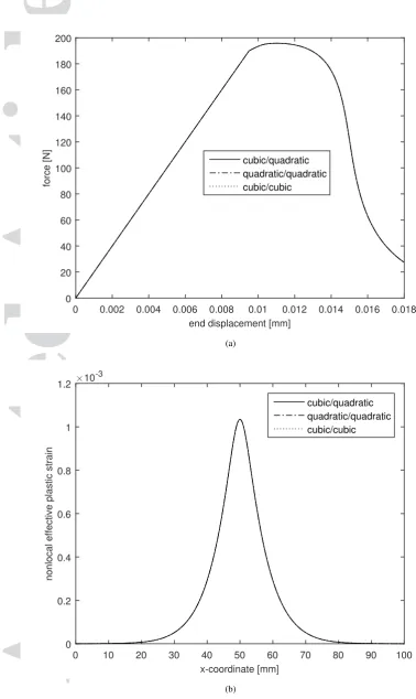
Taking the order of interpolation for the nonlocal effective plastic strain measure to be an order lower than the displacement gives a balanced interpolation. It is useful to investigate the effect of the same orders of interpolation, because when using adaptive or hierarchical refinement, the same order of interpolation may be simpler to implement. Indeed, it has been argued that nonlocal gradient models are coupled problems and the interpolation orders of variables do not have to be balanced [32]. Finally, there are indications from calculations with the second-order explicit gradient plasticity model that stress oscillations can occur in spite of the use of different interpolation orders for the displacements and the plastic multiplier [13].

We consider a one-dimensional bar, which is fixed at one end and subjected to tension at the other end, see Figure 4. The bar has a lengthL= 100 mm, a Young’s modulusE= 20000 N/mm2_{, area}

= 100 mm2_{and an initial tensile strengthσ}

y,0= 2 N/mm2. The tensile strength in the central part

of the bar (21.875mm) is reduced by5%to trigger localisation. A length scaleℓ= 5 mmis used and the bar is discretised with 64 and 128 elements, respectively. Only the second-order implicit gradient plasticity formulation is considered in this section.

Figure 4. Tensile bar with imperfection

A

c

c

e

p

te

d

A

r

ti

c

le

(8), withH= 6000 N/mm2_andκ¯

i= 0, and for an exponential damage evolution, Equation (53),

with H = 6000 N/mm2_{. The critical nonlocal effective plastic strain at full damage ¯κ}

u shows a

significant influence on the linear relation, while β is the dominating parameter when using the exponential relation, cf. [8].

end displacement [mm]

0 0.01 0.02 0.03 0.04 0.05 0.06 0.07 0.08 0.09 0.1

force [N]

0 50 100 150 200 250 300

κu= 3e-4

κu= 6e-4

κu= 9e-4

(a)

end displacement [mm]

0 0.01 0.02 0.03 0.04 0.05 0.06

force [N]

0 50 100 150 200 250

β= 3e3

β= 6e3

β= 9e3

(b)

Figure 5. Influence of material parameters for bar without imperfection discretised with 64 elements using linear (a) and exponential (b) damage evolution law. Results are shown for an interpolation orderp= 2_of

the nonlocal plastic multiplier andp= 3_{of the displacement.}

All subsequent simulations are for the tensile bar with an imperfection. The load-displacement curves are shown in Figure 6 for a quadratic interpolation of the nonlocal plastic multiplier and a cubic interpolation of the displacement. The parametersH = 2000 N/mm2_,κ¯

A

c

c

e

p

te

d

A

r

ti

c

le

are used for linear damage evolution, while H = 9000 N/mm2 _{and β= 4300 are adopted for}

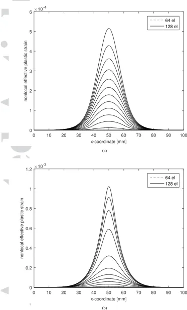
exponential damage evolution. It is clear that mesh-objective results are obtained, since the curves are identical for both discretisations (64 and 128 elements). The evolution of nonlocal effective plastic strain has been plotted in Figure 7. The load-displacement curves as well as the nonlocal effective plastic strain profiles converge throughout the loading history. No visible mesh dependency exists.

end displacement [mm]

0 0.002 0.004 0.006 0.008 0.01 0.012 0.014 0.016 0.018 0.02

force [N]

0 20 40 60 80 100 120 140 160 180 200

lin 64 el lin 128 el exp 64 el exp 128 el

Figure 6. Load-displacement curves using an interpolation orderp= 2 _{for the nonlocal plastic multiplier} andp= 3_{for the displacements. Results are shown for linear and exponential damage evolution relations,}

with 64 and 128 elements.

A

c

c

e

p

te

d

A

r

ti

c

le

x-coordinate [mm]

0 10 20 30 40 50 60 70 80 90 100

nonlocal effective plastic strain

×10-4

0 1 2 3 4 5 6

64 el 128 el

(a)

x-coordinate [mm]

0 10 20 30 40 50 60 70 80 90 100

nonlocal effective plastic strain

×10-3

0 0.2 0.4 0.6 0.8 1 1.2

64 el 128 el

(b)

Figure 7. Evolution of the nonlocal effective plastic strain for linear (a) and exponential (b) damage evolution law with 64 and 128 elements. Results are shown for an interpolation orderp= 2_{of the nonlocal plastic}

A

c

c

e

p

te

d

A

r

ti

c

le

end displacement [mm]

0 0.002 0.004 0.006 0.008 0.01 0.012 0.014 0.016 0.018

force [N]

0 20 40 60 80 100 120 140 160 180 200

cubic/quadratic quadratic/quadratic cubic/cubic

(a)

x-coordinate [mm]

0 10 20 30 40 50 60 70 80 90 100

nonlocal effective plastic strain

×10-3

0 0.2 0.4 0.6 0.8 1 1.2

cubic/quadratic quadratic/quadratic cubic/cubic

(b)

A

c

c

e

p

te

d

A

r

ti

c

le

x-coordinate [mm]

0 10 20 30 40 50 60 70 80 90 100

yield stress [N/mm

2 ]

-2 -1.5 -1 -0.5 0 0.5 1

cubic/quadratic quadratic/quadratic cubic/cubic

(a)

x-coordinate [mm]

0 10 20 30 40 50 60 70 80 90 100

axial stress [N/mm

2 ]

0.26 0.265 0.27 0.275 0.28 0.285 0.29 0.295 0.3 0.305

cubic/quadratic quadratic/quadratic cubic/cubic

(b)

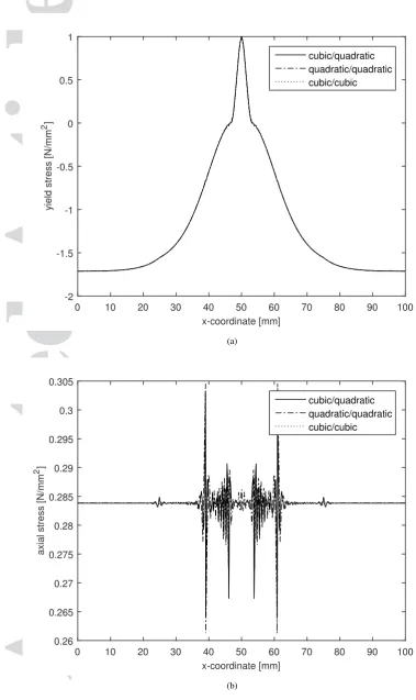
Figure 9. Yield stress (a) and axial stress (b) for different and same interpolation orders for the displacement/nonlocal effective plastic strain. Discretisation is with 128 elements and a exponential damage

A

c

c

e

p

te

d

A

r

ti

c

le

end displacement [mm]

0 0.002 0.004 0.006 0.008 0.01 0.012 0.014 0.016 0.018 0.02

force [N]

0 20 40 60 80 100 120 140 160 180 200

2nd order 64 el 2nd order 128 el 4th order 64 el 4th order 128 el

(a)

x-coordinate [mm]

0 10 20 30 40 50 60 70 80 90 100

nonlocal effective plastic strain

×10-4

-1 0 1 2 3 4 5 6 7

2nd order 64 el 2nd order 128 el 4th order 64 el 4th order 128 el

(b)

A

c

c

e

p

te

d

A

r

ti

c

le

end displacement [mm]

0 0.002 0.004 0.006 0.008 0.01 0.012 0.014 0.016

force [N]

0 20 40 60 80 100 120 140 160 180 200

2nd order 64 el 2nd order 128 el 4th order 64 el 4th order 128 el

(a)

x-coordinate [mm]

0 10 20 30 40 50 60 70 80 90 100

nonlocal effective plastic strain

×10-4

-2 0 2 4 6 8 10 12

2nd order 64 el 2nd order 128 el 4th order 64 el 4th order 128 el

(b)

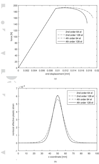
Figure 11. Tensile bar: Load-displacement curves (a) and nonlocal effective plastic strain profiles (b) for second-order and fourth-order gradient formulations discretised with different number of elements. An

A

c

c

e

p

te

d

A

r

ti

c

le

6. COMPARISON OF SECOND-ORDER AND FOURTH-ORDER GRADIENT FORMULATIONS

6.1. One-dimensional bar in tension

We revisit the problem of an imperfect bar subjected to tension discussed in the previous section (Figure 4). We now consider the second-order and the fourth-order implicit gradient plasticity formulations using a cubic interpolation for the displacements and a quadratic interpolation for the nonlocal effective plastic strain. We recall that for the second-order gradient formulation,ca=ℓ2,

cb= 0, and that for the fourth-order formulation ca =ℓ2/2, cb=ℓ4/8. The load-displacement

curves and nonlocal effective plastic strain profiles are shown in Figure 10 for a linear damage evolution.

Convergence is achieved in all cases, but significant differences occur between both formulations. The second-order implicit gradient formulation shows a more ductile response and a broader localisation band than the fourth-order formulation. This supports the results of the dispersion analysis, Figure 2, which point at a broader localisation band for the second-order formulation. The additional term due to the non-zero coefficientcb in the fourth-order formulation leads to a

higher peak of the nonlocal effective plastic strain in the fourth-order formulation, see Figure 10(b). The same trend is observed for the exponential damage evolution law, see Figure 11.

6.2. Square plate under uniaxial tension

Next, the two-dimensional panel is considered shown in Figure 12. The left side is fixed in thex

direction and the midpoint of this side is fixed in theydirection as well. A displacementu¯is imposed on the right side. Regarding the panel dimensions L= 10 mm, and the material properties are

E= 20000 N/mm2_{,H= 2000 N/mm}2_{, andσ}

y,0= 2 N/mm2. An exponential damage evolution

is assumed withβ= 3500and a length scaleℓ= 0.7 mm. The yield strength is reduced by5%at the bottom left corner of the panel to trigger localisation. Three uniformly refined meshes are considered with 256, 1,024 and 4,096 elements, respectively, see Figure 13, with a cubic interpolation for the displacements and a quadratic interpolation for the pressure.

Figure 12. Geometry and boundary conditions of two-dimensional panel subjected to uniaxial tension

A

c

c

e

p

te

d

A

r

ti

c

le

(a) (b)

(c)

Figure 13. Meshes of square panel indicating weakened elements: (a) 256 elements; (b) 1,024 elements; (c) 4,096 elements

displacement [mm] _×10-3

0 0.5 1 1.5 2 2.5 3

force [N]

0 2 4 6 8 10 12 14 16 18 20

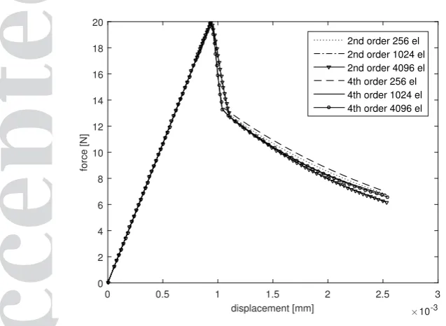
2nd order 256 el 2nd order 1024 el 2nd order 4096 el 4th order 256 el 4th order 1024 el 4th order 4096 el

Figure 14. Load-displacement curves for square panel.

Moreoever, this corroborates the results of the dispersion analysis which indicate that the second-order formulation has a bigger band width. Conversely, for explicit gradient plasticity formulations, shear localisation analyses [33, 34] show a broader localisation band for an explicit second-order gradient model compared to an explicit gradient model with fourth-order gradients.

A

c

c

e

p

te

d

A

r

ti

c

le

0 0.5 1 1.5 2 2.5 3 3.5 4 4.5 5 (a)

×10-4

0 0.5 1 1.5 2 2.5 3 3.5 4 4.5 5 (b)

×10-4

0 0.5 1 1.5 2 2.5 3 3.5 4 4.5 5 (c)

×10-4

0 0.5 1 1.5 2 2.5 3 3.5 4 4.5 5 (d)

×10-4

0 0.5 1 1.5 2 2.5 3 3.5 4 4.5 5 (e)

×10-4

0 0.5 1 1.5 2 2.5 3 3.5 4 4.5 5 (f)

Figure 15. Square panel: Distribution of nonlocal effective plastic strain for the second-order (left) and fourth-order (right) formulations

.

further localisation within the band is observed in Figures 17(e) and 17(f). This is in agreement with results from standard finite element simulations [8].

A

c

c

e

p

te

d

A

r

ti

c

le

x-coordinate [mm]

0 1 2 3 4 5 6 7 8 9 10

nonlocal effective plastic strain

×10-4

-0.5 0 0.5 1 1.5 2 2.5 3 3.5 4 4.5

2nd order 1024 el 2nd order 4096 el 4th order 1024 el 4th order 4096 el

Figure 16. Distribution of nonlocal effective plastic strain along the diagonal AB, cf. Figure 12

implicit gradient plasticity models using standard finite elements [8], meshless methods [13] and isogeometric analysis [14]. The angle of the shear band is lower than 45owhich is the theoretical solution for a shear band when using a Tresca plasticity model. Unlike for the Tresca yield function, the intermediate principal stress enters the Von Mises yield condition, and this results in a different condition for the onset of localisation, including the angle of shear bands, cf. [35]. It is finally noted that the curving upward of the shear band near the free boundary is related to the emergence of stationary Rayleigh waves [36], and has been observed in other simulations as well [37].

6.3. Biaxially compressed specimen

To further assess the capability of the model, a biaxially compressed plane-strain specimen is considered, Figure 18, cf. [12, 8]. The width L= 10 mm. All material parameters are as in the previous section except that nowβ= 2500andν= 0.3. The elements with reduced yield strength (by 5%) are shown in Figure 19.

A

c

c

e

p

te

d

A

r

ti

c

le

×10-4

0 0.1 0.2 0.3 0.4 0.5 0.6 0.7 0.8 0.9 1

(a)

×10-4

0 0.1 0.2 0.3 0.4 0.5 0.6 0.7 0.8 0.9 1

(b)

×10-4

0 0.1 0.2 0.3 0.4 0.5 0.6 0.7 0.8 0.9 1

(c)

×10-4

0 0.1 0.2 0.3 0.4 0.5 0.6 0.7 0.8 0.9 1

(d)

×10-4

0 0.1 0.2 0.3 0.4 0.5 0.6 0.7 0.8 0.9 1

(e)

×10-4

0 0.1 0.2 0.3 0.4 0.5 0.6 0.7 0.8 0.9 1

(f)

Figure 17. Evolution of the local (left) and the nonlocal (right) effective plastic strain at maximum displacement:u¯= 0.00093 mm_{– (a), (b);}u¯= 0.00096 mm_{– (c), (d);}u¯= 0.001 mm_{– (e), (f)}

A

c

c

e

p

te

d

A

r

ti

c

le

Figure 18. Biaxially compressed specimen: (a) geometry and boundary.

(a) (b) (c)

A

c

c

e

p

te

d

A

r

ti

c

le

displacement [mm] _×10-3

0 0.5 1 1.5 2 2.5 3 3.5

force [N]

0 2 4 6 8 10 12 14 16 18 20

2nd order 200 el 2nd order 800 el 2nd order 3200 el 4th order 200 el 4th order 800 el 4th order 3200 el

A

c

c

e

p

te

d

A

r

ti

c

le

×10-4

0 0.5 1 1.5 2 2.5 3 3.5 4 4.5 5

(a)

×10-4

0 0.5 1 1.5 2 2.5 3 3.5 4 4.5 5

(b)

×10-4

0 0.5 1 1.5 2 2.5 3 3.5 4 4.5 5

(c)

×10-4

0 0.5 1 1.5 2 2.5 3 3.5 4 4.5 5

(d)

×10-4

0 0.5 1 1.5 2 2.5 3 3.5 4 4.5 5

(e)

×10-4

0 0.5 1 1.5 2 2.5 3 3.5 4 4.5 5

(f)

Figure 21. Biaxial compression: Distribution of nonlocal effective plastic strain for the second-order (left) and fourth-order (right) formulations.

A

c

c

e

p

te

d

A

r

ti

c

le

The introduction of strain softening in plasticity models leads to a loss of well-posedness of the boundary value problem. Various approachs to regularise the problem exist, such as the use of nonlocal models, either in an integral sense by spatial averaging, or in a differential sense, by including higher-order spatial gradients of a history variable. It is now well established that both approaches are closely related [10].

Computationally, the addition of gradients is preferred, since in this approach a sparse, banded stiffness matrix is preserved, and it is possible to retain symmetry of the tangential stiffness matrix, which is different from nonlocal integral approaches [38]. Explicit second-order gradient plasticity models properly regularise the boundary value problem, as has been shown by dispersion analyses, and one-dimensional and two-dimensional finite element analyses of localisation. However, in explicit gradient plasticity the interpolation of the plastic multiplier must satisfyC1_{-continuity, since}

this is a necessary condition at the moving, internal elasto-plastic boundary [3]. This degree of continuity is difficult to satisfy using finite element approaches, and alternative formulations have been put forward [12, 13, 14].

The use of a second-order implicit gradient plasticity model, in which the nonlocal plastic strain is interpolated [8], is an alternative way to solve this issue since a C0_{-continuous interpolation}

for the nonlocal plastic equivalent strain suffices. However, it does not rigorously regularise the boundary value problem [17]. In this paper we have explored the use of a fourth-order implicit gradient plasticity model. A dispersion analysis and one-dimensional and two-dimensional numerical analyses show that a regularisation, with mesh-independent results, can be obtained. Unfortunately, as with the explicit second-order gradient plasticity model, this requires a C1

-continuous interpolation, now for the nonlocal plastic strain. Herein, it has been proposed to exploit isogeometric finite element analysis to meet this requirement.

It depends on the chosen damage relation whether the width of the localisation band tends to zero, thus resulting in a sharp crack, but also in a local loss of ellipticity. This is not different from the situation for second-order implicit gradient plasticity, but marks a clear difference with that for the second-order explicit gradient-plasticity model.

A

c

c

e

p

te

d

A

r

ti

c

le

Box 1. Algorithm for implicit gradient plasticity formulations (iterationj+ 1)

1. Compute the matrices Kaa, Kaλ, Kλa and Kλλ, and forces fe, fa and fλ, according to

Equations (69) – (74)

2. Solve fordaandd ¯Λusing Equation (68)

3. Update the total increments∆aj+1= ∆aj+ da, and∆Λj+1= ∆Λj+ dΛ.

4. Compute the following at each integration point:

∆εεεj+1=B∆aj+1,

∆¯λj+1 =hT∆ ¯Λj+1,

∇(∆λj+1) =QT∆Λj+1,

∇2_(∆λ

j+1) =pT∆Λj+1, ¯

κj+1= ¯κ0+ ∆λj+1,

∇κ¯j+1=∇¯κ0+∇(∆¯λj+1),

∇2_κ¯

j+1=∇2κ¯0+∇2(∆¯λj+1),

computeωj+1according to adopted damage evolution law

trial stressσσσt=σσσ0+De∆εεεj+1.

IfF(σσσt, κ0,κ¯j+1)>1×10−6,

then plastic state: computemt

compute∆γj+1 κj+1=κ0+ ∆γj+1,

compute the algorithmic stiffness operatorA

update the trial stress update according to Equation (38) else

elastic state: mt=0

σ σ

σj+1=σσσt

A=De

5. Check the global convergence criterion. If not converged, go to 1.

(•)0denotes value at previous converged load step and(•)jindicates value at previous iteration.

REFERENCES

1. Zdenˇek P Baˇzant, Ted B Belytschko, and Ta-Peng Chang. Continuum theory for strain-softening. Journal of Engineering Mechanics, 110:1666–1692, 1984.

2. Zdenˇek Baˇzant and Feng-Bao Lin. Non-local yield limit degradation. International Journal for Numerical Methods in Engineering, 26:1805–1823, 1988.

3. Ren´e de Borst and Hans-Bernd M¨uhlhaus. Gradient-dependent plasticity: Formulation and algorithmic aspects.

International Journal for Numerical Methods in Engineering, 35:521–539, 1992.

4. H-B M¨uhlhaus and E C Alfantis. A variational principle for gradient plasticity. International Journal of Solids and Structures, 28:845–857, 1991.

5. R de Borst, L J Sluys, H-B M¨uhlhaus, and Jerzy Pamin. Fundamental issues in finite element analyses of localization of deformation. Engineering Computations, 10:99–121, 1993.

6. R H J Peerlings, R de Borst, W A M Brekelmans, and J H P de Vree. Gradient enhanced damage for quasi-brittle materials. International Journal for Numerical Methods in Engineering, 39:3391–3403, 1996.

7. Harm Askes, Jerzy Pamin, and Ren´e de Borst. Dispersion analysis and element-free Galerkin solutions of second-and fourth-order gradient-enhanced damage models. International Journal for Numerical Methods in Engineering, 49:811–832, 2000.

8. Roy A B Engelen, Marc G D Geers, and Frank P T Baaijens. Nonlocal implicit gradient-enhanced elasto-plasticity for the modelling of softening behaviour. International Journal of Plasticity, 19:403–433, 2003.

A

c

c

e

p

te

d

A

r

ti

c

le

10. R H J Peerlings, M G D Geers, R de Borst, and W A M Brekelmans. A critical comparison of nonlocal and gradient-enhanced softening continua. International Journal of Solids and Structures, 38:7723–7746, 2001. 11. T. H. A. Nguyen, T. Q. Bui, and S. Hirose. Smoothing gradient damage model with evolving anisotropic nonlocal

interactions tailored to low-order finite elements. Computer Methods in Applied Mechanics and Engineering, 328:498–541, 2018.

12. Rene de Borst and Jerzy Pamin. Some novel developments in finite element procedures for gradient-dependent plasticity. International Journal for Numerical Methods in Engineering, 39:2477–2505, 1996.

13. Jerzy Pamin, Harm Askes, and Ren´e de Borst. Two gradient plasticity theories discretized with the element-free Galerkin method. Computer Methods in Applied Mechanics and Engineering, 192:2377–2403, 2003.

14. I. Kolo and R. de Borst. An isogeometric analysis approach to gradient plasticity. International Journal for Numerical Methods in Engineering, DOI: 10.1002/nme.5614.

15. R de Borst, J Pamin, R H J Peerlings, and L J Sluys. On gradient-enhanced damage and plasticity models for failure in quasi-brittle and frictional materials. Computational Mechanics, 17:130–141, 1995.

16. Giovanni Di Luzio and Zdenˇek P Baˇzant. Spectral analysis of localization in nonlocal and over-nonlocal materials with softening plasticity or damage. International Journal of Solids and Structures, 42:6071–6100, 2005. 17. L H Poh and S Swaddiwudhipong. Gradient-enhanced softening material models. International Journal of

Plasticity, 25:2094–2121, 2009.

18. Xilin Lu, Jean-Pierre Bardet, and Maosong Huang. Spectral analysis of nonlocal regularization in two-dimensional finite element models. International Journal for Numerical and Analytical Methods in Geomechanics, 36:219–235, 2012.

19. Milan Jir´asek and Simon Rolshoven. Comparison of integral-type nonlocal plasticity models for strain-softening materials. International Journal of Engineering Science, 41:1553–1602, 2003.

20. Milan Jir´asek and Simon Rolshoven. Localization properties of strain-softening gradient plasticity models. Part II: Theories with gradients of internal variables. International Journal of Solids and Structures, 46:2239–2254, 2009. 21. R A B Engelen, N A Fleck, R H J Peerlings, and M G D Geers. An evaluation of higher-order plasticity theories for predicting size effects and localisation. International Journal of Solids and Structures, 43:1857–1877, 2006. 22. Thomas J R Hughes, John A Cottrell, and Yuri Bazilevs. Isogeometric analysis: CAD, finite elements, NURBS,

exact geometry and mesh refinement. Computer Methods in Applied Mechanics and Engineering, 194:4135–4195, 2005.

23. Michael J Borden, Michael A Scott, John A Evans, and Thomas J R Hughes. Isogeometric finite element data structures based on B´ezier extraction of NURBS. International Journal for Numerical Methods in Engineering, 87:15–47, 2011.

24. R. de Borst, M. A. Crisfield, J. J. C. Remmers, and C. V. Verhoosel. Non-linear Finite Element Analysis of Solids and Structures. John Wiley & Sons, Chichester, second edition, 2012.

25. R H J Peerlings, R de Borst, W A M Brekelmans, J H P de Vree, and I Spee. Some observations on localisation in non-local and gradient damage models. European Journal of Mechanics A: Solids, 15:937–953, 1996.

26. Gerald Beresford Whitham. Linear and Nonlinear Waves. John Wiley & Sons, New York, 1974.

27. L J Sluys, R de Borst, and H-B M¨uhlhaus. Wave propagation, localization and dispersion in a gradient-dependent medium. International Journal of Solids and Structures, 30:1153–1171, 1993.

28. L J Sluys and R de Borst. Dispersive properties of gradient-dependent and rate-dependent media. Mechanics of Materials, 18:131–149, 1994.

29. M. G. Cox. The numerical evaluation of B-splines. IMA Journal of Applied Mathematics, 10:134–149, 1972. 30. C. de Boor. On calculating with B-splines. Journal of Approximation Theory, 6:50–62, 1972.

31. Julien Vignollet, Stefan May, and Ren´e de Borst. Isogeometric analysis of fluid-saturated porous media including flow in the cracks. International Journal for Numerical Methods in Engineering, 108:990–1006, 2016.

32. A Simone, H Askes, R H J Peerlings, and L J Sluys. Interpolation requirements for implicit gradient-enhanced continuum damage models. International Journal for Numerical Methods in Biomedical Engineering, 19:563– 572, 2003.

33. A Menzel and P Steinmann. On the continuum formulation of higher gradient plasticity for single and polycrystals.

Journal of the Mechanics and Physics of Solids, 48:1777–1796, 2000.

34. Xue-Bin Wang. Adiabatic shear localization for steels based on Johnson-Cook model and second- and fourth-order gradient plasticity models. Journal of Iron and Steel Research, International, 14:56–61, 2007.

35. J. W. Rudnicki and J. R. Rice. Conditions for the localization of deformation in pressure-sensitive dilatant materials.

Journal of the Mechanics and Physics of Solids, 23:371–394, 1975.

36. A. Needleman and M. Ortiz. Effect of boundaries and interfaces on shear-band localization. International Journal of Solids and Structures, 28:859–877, 1991.

37. R. de Borst, J. R´ethor´e, and M. A. Abellan. A numerical approach for arbitrary cracks in a fluid-saturated medium.

Archive of Applied Mechanics, 75:595–606, 2006.

38. G. Pijaudier-Cabot and A. Huerta. Finite element analysis of bifurcation in nonlocal strain softening solids.