Multi arrival wavefront tracking and seismic imaging

and Seismic Imaging

J¨

urg Hauser

October 2007

This thesis contains no material which has been accepted for the award of any other degree or diploma in any university or institution. To the best of my knowledge this thesis contains no material previously published or written by another person except where due reference is made in the text.

Acknowledgements

This work would not have succeeded without the assistance and support of those people around me.

First and foremost I would like to thank Dr. Malcolm Sambridge and Dr. Nick Rawlinson. This thesis greatly benefited from their knowledge, support and en-couragement. Their guidance and unfailing high standards significantly improved the end product.

The feedback provided by Prof. Brian Kennett on the occasion of my midterm review was invaluable.

I wish to thank Prof. Douglas Wiens for providing a copy of the velocity model for the seismic structure beneath the Tonga arc and Lau backarc basin.

Abstract

Multi Arrival Wavefront Tracking and Seismic Imaging

Multi valued travel times have traditionally not been used in seismic imaging, with only a handful of notable exceptions in the field of exploration geophysics. For studies on local and regional scales (e.g. local earthquake/teleseismic tomography), the focus has largely been on first arrivals. Numerous ray and grid based schemes have been developed for predicting this class of data. However, later arrivals often contribute to the length and shape of a recorded wavetrain, particularly in regions of complex geology. These arrivals are likely to contain additional information about seismic structure, as their two point path differs from that of the first arrival; in particular, they are more amenable to sampling regions of lower velocity.

Recently, several grid based schemes have been proposed for solving the multi valued travel time problem. Here a level set based scheme is investigated for its po-tential to accurately and robustly compute travel times in a seismological context. Although promising, it is shown that it, and other grid based multi arrival solvers, currently require significant computational resources for crustal scale problems, and further development is required before practical application becomes feasible. The main focus of this work is therefore on an alternative approach, sometimes referred to as wavefront construction. The wavefront construction principle is used as the basis of a new scheme for computing multi valued travel times that arise from smooth variations in both velocity structure and interface geometry. The idea is to represent the wavefront as a set of points, and use local ray tracing and interpolation to advance the wavefront in a series of time steps. The wavefront tracking is performed in reduced phase space, which significantly enhances the method’s ability to correctly resolve complex features such as triplications. The scheme is robust in the presence of strong velocity heterogeneity and interface cur-vature, with phases comprising multiple reflections, refractions and triplications successfully tracked.

1 Introduction 1

1.1 Motivation . . . 1

1.2 Ray based methods . . . 3

1.3 Grid based methods . . . 6

1.3.1 First arrival schemes . . . 6

1.3.2 Multi arrival schemes . . . 10

1.4 Wavefront tracking . . . 13

1.5 Outline . . . 15

2 Eulerian scheme 17 2.1 Formulation of interface propagation . . . 18

2.2 Level set method . . . 19

2.2.1 Level set equation . . . 20

2.2.2 Signed distance function . . . 21

2.2.3 Basic algorithm for interface evolution . . . 22

2.2.3.1 Solution in one dimensional space . . . 23

2.2.3.2 Solution in a higher dimensional space . . . 27

2.2.3.3 Higher order finite difference operator . . . 30

2.2.3.4 Numerical realisation . . . 34

2.2.4 Improved algorithms for interface propagation . . . 36

2.2.4.1 Reinitialisation . . . 37

2.2.4.2 Narrow band approach . . . 40

2.2.5 Three dimensions . . . 43

2.3 Reduced phase space . . . 44

2.4 Propagating the bicharacteristic strip in an Eulerian framework . . 46

2.4.1 Arrival time extraction . . . 48

2.5.1 Constant velocity . . . 50

2.5.2 Wave guide structure . . . 51

2.5.3 Subduction zone . . . 54

2.6 Summary . . . 56

3 Lagrangian scheme 59 3.1 Wavefront tracking in reduced phase space . . . 59

3.1.1 Local wavefront refinement . . . 61

3.1.2 Extracting arrival information . . . 65

3.1.3 Dynamic ray tracing . . . 67

3.2 Examples . . . 70

3.2.1 Constant velocity . . . 71

3.2.2 Constant velocity gradient . . . 72

3.2.3 Subduction zone . . . 76

3.2.4 Marmousi model . . . 79

3.2.5 Surface wave multipathing . . . 82

3.3 Summary . . . 86

4 Extensions of the Lagrangian scheme 89 4.1 Interfaces . . . 89

4.1.1 Representation of an interface . . . 90

4.1.2 Wavefront propagation in the presence of interfaces . . . 92

4.1.3 Ray path extraction in the presence of interfaces . . . 96

4.2 Gaussian beam method . . . 98

4.2.1 Gaussian beams in smoothly varying media . . . 99

4.2.2 Reflection and refraction of Gaussian beams . . . 106

4.3 Examples . . . 111

4.3.1 Global travel time model . . . 111

4.3.2 Receiver functions . . . 117

4.4 Summary . . . 123

5 Seismic tomography with later arrivals 125 5.1 Objective function . . . 127

5.2 Subspace method . . . 129

5.3 Fr´echet matrix . . . 132

5.4 Including later arrivals in tomography . . . 133

5.4.2 Layered velocity model . . . 141

5.5 Summary . . . 151

6 Multi valued travel times in three dimensions 153 6.1 Representing the wavefront . . . 154

6.1.1 Surface refinement . . . 157

6.1.2 Surface simplification . . . 162

6.1.3 Mesh quality . . . 164

6.1.4 Extracting arrival information . . . 171

6.2 Examples . . . 175

6.2.1 Constant velocity gradient . . . 175

6.2.2 Complex structure . . . 178

6.2.3 SEG/EAGE Salt dome model . . . 180

6.3 Summary . . . 184

7 Conclusions 187 Bibliography 193

Appendices

D.2 Fr´echet derivative for an interface node . . . 225

E Contents of enclosed CD 227 E.1 Animations . . . 227

Introduction

1.1

Motivation

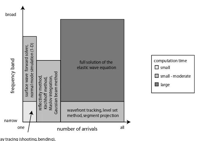
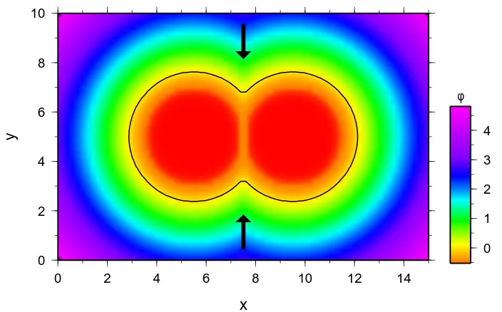
Both continuous and discontinuous variations in wave speed can cause seismic en-ergy to travel to a receiver along more than one path, a phenomenon commonly referred to as multipathing. This is illustrated in figure 1.1 where a wavefront trip-licates due to the presence of a low velocity anomaly, resulting in the detection of three separate arrivals at the receiver. The shape of the self-intersecting wavefront at time t+ ∆tresembles what is often described as a swallowtail. The first arrival path avoids the low velocity anomaly, which is subsequently sampled by the second and third arrival. Clearly, later arrivals sample different parts of the medium and therefore should carry additional structural information. However, current state of the art algorithms for tracking wavefronts or rays only provide the travel times of first arrivals (e.g. Rawlinson & Sambridge, 2004a; Buske & K¨astner, 2004; de Kool et al., 2006). The development of advanced and computationally practical schemes for tracking multiple arrivals through complex two and three dimensional media would allow the prediction of a far greater proportion of the seismic wavefield, which has the potential to benefit many areas of seismology. For example, seismic imaging schemes which also exploit later portions of the recorded wavetrain could result in more detailed and accurate maps of earth structure. Figure 1.2 shows an idealised schematic plot of how multi arrival wavefront tracking compares to other common seismic wave simulation techniques with regard to representation of frequency and arrival information. While it can predict all arrivals, it is limited to the high frequency approximation of the wave equation.

wavefront at time wavefront at time faster slower time source receiver

Figure 1.1: Schematic diagram showing ray paths for a medium containing a slow velocity anomaly. The wavefront triplicates and three arrivals are observed. The ray path for the first, second and third arrivals are shown in red, green and blue, respectively.

number of arrivals

fr

eq

ue

nc

y b

and _{elastic wave equation}full solution of the

wavefront tracking, level set method, segment projection

sur fac e w av e f or wa rd s o lv e r, nor m al mo de s imu la tio n ( 1-D)

ray tracing (shooting, bending), eikonal solvers, shortest path methods

broad

narrow

one all

small

small - moderate

large computation time re flec tivi ty met ho d , Ki rchh off me tho d, Ma slo v in te g ra tio n , Ga u ssian b ea m me tho d

of the elastic wave equation (e.g. Kelly et al., 1976; Graves, 1996; Komatitsch & Tromp, 1999; Bohlen, 2002) provide synthetic seismograms which already contain later arrivals, and hence there is no need for a high frequency approach. However, numerical solution of the full wave equation is computationally expensive and significant challenges confront its use in seismic imaging. While it is true that recent developments involving adjoint methods and scattering integral methods allow path sensitivity information to be extracted (e.g. Tromp et al., 2005; Chen et al., 2007a) and used in the gradient based inversion of the synthetic waveform, many issues, including non-linearity, stability and computation time, are yet to be resolved (e.g. Tape et al., 2007; Chen et al., 2007b).

The calculation of ray travel times through a medium with a heterogeneous velocity distribution still remains the foundation of many applications that rely on the high frequency component of seismic records, such as body wave tomography, migration of reflection data and earthquake relocation (e.g. Thurber, 1983; Gray & May, 1994; Hammer et al., 1994; Steck et al., 1998). Despite many decades of technique development (e.g. Julian & Gubbins, 1977; Vidale, 1988; Sethian & Popovici, 1999), there is still no single method that can accurately, efficiently and robustly overcome the non-linearity of the two point problem, and compute all multi arrivals in complex media. The aim of this thesis is to advance the current state of the art in seismic wavefront tracking in heterogeneous media, and to investigate the potential of multi arrival information for improving various seismic applications including tomography.

1.2

Ray based methods

syn-−40 −30 −20 −10 0

depth (km)

0 10 20 30 40 50 60 70 80 90 100

horizontal distance (km)

1 2 3 4 5 6 7 8 9 km/s

Figure 1.3: Rays generated by a uniform fan of 300 rays emitted from a source point (black star) in a smoothly varying heterogeneous velocity model. The angular distance between all adjectant paths is the same at the source. This relationship is no longer preserved as the rays are traced through the structure. Two rays with similar initial directions but very different overall geometries are marked in green and blue.

thetic seismograms based on these properties. For a layered structure one can use the reflection matrix approach of Kennett (1983) which allows the computation of a synthetic seismogram based on travel times and reflection and transmission coefficients at the interfaces. If geometrical spreading factors are computed and the number of caustics is known in advance, then the Maslov integration method can be applied (e.g. Chapman, 1985). Another approach is the so called Gaussian beam method of ˇCerven´y & Pˇsenˇc´ık (1984), which does not require the number of caustics along a ray to be known. It is also possible to take attenuation into account by computing a dissipation factor and convolving it with the seismogram (e.g. Weber, 1988).

The real challenge of boundary value ray tracing is to determine the initial direction vector of the ray that will hit a particular receiver. This two point problem of finding a source-receiver ray path can be formulated as an inverse problem, in which the unknown is the initial direction vector of the ray, and the function to be minimised is a measure of the distance between the ray endpoint and receiver. Since the optimisation problem is linear, a range of iterative non-linear and fully non-non-linear schemes has been employed (e.g. Julian & Gubbins, 1977; Sambridge & Kennett, 1990; Virieux & Farra, 1991; Velis & Ulrych, 1996).

sector of the model (horizontal distance x >85 km and depthz >₋20 km). There is significant defocusing of rays heading in this direction due to the fast region to the right of the source. Several rays end up propagating in a direction which differs by up to 180◦ _{from their initial direction. One commonly refers to these} as overturning rays (see green ray in figure 1.3). Small changes in the initial ray direction also have the potential to cause significant changes in the geometry of the resulting ray path (cf. the green and blue rays in figure 1.3)

in the temperature parameter, but in practice a finite step has to be used. Velis & Ulrych (2001) extend the method to three dimensions and implement a ver-satile model parameterization scheme. However their approach does not appear to be practical for finding all multipaths, and tends to be more computationally expensive than iterative non-linear solvers.

An alternative to ray shooting is to begin with an arbitrary initial path, and then iteratively adjust its geometry until it becomes a true ray path (i.e. it satis-fies Fermat’s principle of stationary time). A common approach to implementing this so called bending method is to derive a boundary value formulation of the kinematic ray tracing equations, which can then be solved iteratively (e.g. Julian & Gubbins, 1977). However, as in the shooting method the resulting ray path is not necessarily the first arrival ray path, as the technique cannot distinguish between a local an global extrema. This could be overcome if a fully non-linear search is used, but such an approach is likely to encounter similar limitations to the simulated annealing shooting scheme of Velis & Ulrych (1996, 2001). Pereyra et al. (1980) extend the ray bending technique so that interfaces can be included, and use shooting to obtain an initial ray path. They use a separate system of equations for each layer and couple them by applying the known discontinuity condition at each interface that is traversed by the ray path. In ray bending, a common method for obtaining a good initial guess for the ray path is to use the two point path from a laterally averaged version of the model (e.g. Thurber & Ellsworth, 1980; Sambridge & Kennett, 1990).

Ray tracing has been widely used in seismic tomography (see Iyer & Hirahara (1993) and Rawlinson & Sambridge (2003) for a comprehensive range of exam-ples); specific applications include imaging the structure between boreholes (e.g. Bregman et al., 1989), the source area of earthquakes (e.g. Zhao et al., 1996a), subducting slabs (e.g. Conder & Wiens, 2006) and mantle upwelling (e.g. Toomey et al., 1998).

1.3

Grid based methods

1.3.1

First arrival schemes

field implicitly contains the wavefront location as a function of time (i.e. isochrons of the travel time field), and all possible first arrival ray paths are given by the gradient of the travel time field. Grid based methods have evolved to the point where many can guarantee to locate the first arrival travel time and ray path to all points of the medium (e.g. Rawlinson & Sambridge, 2004a; Buske & K¨astner, 2004), even for highly heterogeneous media, where ray tracing is likely to fail. In figure 1.4, wavefronts have been computed using a finite difference eikonal solver for the same velocity model through which rays have been traced in figure 1.3. The wavefronts extracted from the travel time field appear to be stable despite the strong heterogeneity that causes significant focusing and defocusing of the rays. The last 15 years has seen the development of numerous grid based algorithms for efficient computation of arrival times using various finite difference solutions of the eikonal equation. One of the first attempts to compute the first arrival travel time field using a finite difference technique was made in two dimensions by Vidale (1988) who later extended it to three dimensions (Vidale, 1990). The scheme involves progressively integrating travel times along an expanding square in two dimensions or an expanding cube in three dimensions. However, the use of an expanding square to the define the shape of the computational front cannot always respect the direction of flow of travel time information. Hole & Zelt (1995) implement an iterative post sweeping scheme to help account for the non causal nature of the expanding square. Such an idea was first introduced by Schneider et al. (1992). During post sweeping, the travel time field is recomputed several times in different directions, to account for changes in the flow of travel time information caused by velocity heterogeneity. For a two dimensional structure one iteration of the post sweeping procedure involves computing a travel time field starting at the four boundaries of the computational domain. At each grid node the minimum between the newly computed solution and the last updated solution is chosen. Kim & Cook (1999) apply post sweeping in their scheme until the travel time field converges (i.e. the values of the travel time do not change significantly in future applications of the post sweeping steps). They conclude that two applications of their post sweeping procedure leads to sufficiently accurate travel times in their examples.

−40 −30 −20 −10 0

depth (km)

0 10 20 30 40 50 60 70 80 90 100

horizontal distance (km)

1 2 3 4 5 6 7 8 9 km/s

Figure 1.4: First arrival wavefronts calculated using an approach in which the travel time is computed along the boundaries of an expanding box with a fifth order WENO scheme and post sweeping. The algorithm used here is similar to the one described by Kim & Cook (1999). The velocity model is the same as in figure 1.3, and wavefronts are contoured at 1 s intervals.

therefore given by the viscous solution. The weighted essentially non oscillatory scheme (WENO) is a modification of the ENO scheme and has some advantages as far as computation time and stability are concerned (Liu et al., 1994; Jiang & Shu, 1996; Jiang & Peng, 2000).

therefore has the potential to improve accuracy.

Another popular method for determining first arrival travel times at all points of a gridded velocity model is the shortest path method (e.g. Nakanishi, 1985; Moser, 1991; Cheng & House, 1996). In essence, this is an application of graph theory to the problem of ray tracing (e.g. Bondy & Murty, 1976). Seismic ray paths are computed by calculating the shortest travel time path through a network, which represents the velocity medium, using Dijkstra-like algorithms (Dijkstra, 1959). According to Fermat’s principle the path taken between two points by a ray (e.g. light or a seismic wave) corresponds to an extremum (minimum or maximum) of the travel time. This means that the shortest time path between two points is a true ray path. In seismic imaging, shortest path ray tracing has been used by Nakanishi & Yamaguchi (1986) in local earthquake tomography, and Toomey et al. (1994) in the inversion of three dimensional refraction data. So called hybrid methods based on the graph method and ray bending have been used to image crustal structure (e.g. Korenaga et al., 2000). In this context the shortest path method is used to compute an initial ray path for a bending method. Another technique for computing the travel time of first arrivals is the fast marching method (e.g. Sethian & Popovici, 1999) or FMM, which is an Eulerian (i.e. grid based) wavefront evolution method that solves the eikonal equation using upwind finite differences. When compared with the previous finite difference tech-niques, FMM is able to compute correct travel times for overturning rays and can be implemented with unconditional stability (Sethian & Popovici, 1999). Kim & Cook (1999) claim that their grid based scheme is also unconditionally stable. In the case of FMM, the unconditional stability comes from the use of upwind entropy satisfying operators which are well behaved in the presence of discontinuities in the first arrival travel time field, together with a narrow band evolution technique that always satisfies causality. FMM can be extended to handle interfaces and hence the computation of travel times for refracted and reflected waves (Rawlinson & Sambridge, 2004b; de Kool et al., 2006).

is to reinitialise the computational front from the point of minimum travel time on the interface. As a consequence, separate travel time fields do not need to be computed for the receivers (e.g. Li & Ulrych, 1993; Rawlinson & Sambridge, 2004a,b), but it is no longer possible to compute multiple reflection paths.

As mentioned above, important advantages of grid based algorithms, and in particular FMM, compared to traditional ray tracing, are their computational efficiency, algorithmic simplicity, robustness and solution completeness, as long as the arrival time is single valued. If required, wavefronts and rays can be obtained a posteriori by either contouring the travel time field or following the travel time gradient from receiver to source, respectively (e.g. Rawlinson & Sambridge, 2004a; de Kool et al., 2006)

In the field of applied mathematics these schemes, where an actual travel time field is computed on a mesh of points, are commonly known as Eulerian methods (e.g. Sethian, 1999), as the propagation of the wavefront is described by computing its arrival time at the nodes of a fixed underlying grid. These grid based schemes have been used in a variety of seismological applications, and are particularly useful if large travel time datasets have to be computed, such as in seismic tomography (e.g. Rawlinson et al., 2006a,b) or the migration of coincident reflection sections (e.g. Gray & May, 1994; Bevc, 1997; Popovici & Sethian, 2002). However, if later arrivals are required, the methods discussed above are no longer appropriate.

1.3.2

Multi arrival schemes

The question of whether or not first arrivals are sufficient for imaging complex structures was posed soon after the appearance of first arrival finite difference techniques. In the context of exploration geophysics, Geoltrain & Brac (1993) conjectured that most of the wavefield energy is contained in later arrivals and therefore first arrival travel times are not sufficient to give a good migration image. There have been attempts to compute multi valued travel time fields using only a first arrival solver. However, these schemes often include a rather ad hoc procedure for dividing the computational domain into single valued subregions, followed by application of a first arrival solver in each subregion. The solutions for the different subregions are then superimposed to construct the multi valued travel time field (e.g. Fatemi et al., 1995; Benamou, 1999).

take advantage of the work of Osher & Sethian (1988), who pioneered the field of interface tracking. A wavefront at a certain moment in time can be interpreted as an interface between points of a grid which have been crossed by the wavefront and points which have not yet been crossed (i.e. an iso-contour of the travel time field). Their idea was to replace ray tracing (i.e. solving ordinary differential equations for Lagrangian trajectories and other associated Lagrangian variables), with the computation of Eulerian variables, (i.e. the solution of partial differential equations on a grid). To do this they developed the level set method, which keeps track of an interface by expressing it as the zero level set (zero contour line) of a function representing the signed distance to the interface. A signed distance function is an Eulerian variable used to describe the position of an interface. Its value at a certain node of an underlying grid is given by the distance to the closest point on the interface. The sign is used to determine on which side of the interface the node is located. For a closed interface the signed distance function is typically defined to be negative for points inside and positive for points outside of the interface. A signed distance function is an implicit description of an interface; its position is given by the zero iso-contour line or zero level set of the signed distance function. This is similar to a travel time field where the wavefronts are given by the isochrons. The concept of a signed distance function is discussed in much more detail in section 2.2.2.

The interface can be implicitly tracked by numerically solving a partial differ-ential equation that describes the evolution of the signed distance function on a grid. Interfaces cannot intersect each other, but they can merge like rain drops on a smooth surface. This means that it is not possible to describe a wavefront swallowtail using the level set method directly; only the first arrival part of the wavefront can be described. The level set method has become the state of the art algorithm for the description of the evolution of interfaces between fluids and gases in two dimensions (e.g. Mulder et al., 1992; Sussman et al., 1994; Chang et al., 1996). If an interface crosses each cell of a grid only once (e.g. like a flame front or the first arriving part of a wavefront) the level set method can be formulated much more efficiently as a boundary value problem, in which time becomes the de-pendent variable, leading to the fast marching method (Sethian, 1999), discussed in the previous section.

The state of a particle on a wavefront is characterised by its position vector x

real space or normal space. One can also define a phase space, which is spanned by components of the position vector and slowness vector. Phase space is part of the Hamiltonian formulation of ray theory (e.g. Chapman, 1985; Lambar´e et al., 1996). Rays in normal space are then replaced by bicharacteristics in phase space (e.g. Chapman, 1985). A three dimensional reduced phase space can be created from two dimensional normal space by simply using the direction θ of the local wavefront normal as the third coordinate. The wavefront is unfolded into a smooth curve, which is sometimes referred to as a bicharacteristic strip (Osher et al., 2002). One reason for referring to this phase space representation of the wavefront as a bicharacteristic strip is due to the fact that it is defined by the bicharacteristics of the eikonal equation, which are the phase space equivalent of the characteristics of the eikonal equation in real space, which correspond to rays. The advantage of phase space or reduced phase space is that when the wavefront self intersects and contains sharp corners, its corresponding bicharacteristics curve will be locally smooth and single valued.

In order to use the level set method to track multi arrival wavefronts, Os-her et al. (2002) describe the bicharacteristic strip in reduced phase space as the intersection of the zero level sets of two three dimensional functions. Engquist & Runborg (2003) devise the so called segment projection method, in which the bicharacteristic strip is represented as a set of segments. This scheme can be viewed as a compromise between explicit wavefront tracking (see next section) and the level set method. The segments are evolved independently on individual grids and the connectivity between segments is handled by interpolation. A more recent study by Qian & Leung (2004) uses the level set method for the computation of multi valued travel times that satisfy the paraxial wave equation.

Fomel & Sethian (2002) use the Liouville formulation of the ray tracing equa-tions, a system of time independent partial differential equations (referred to as escape equations), which can be solved numerically on a grid in reduced phase space. The solutions correspond to arrival times at the boundary from every point in the phase space domain. Multi arrival information such as wavefront geometry and two point travel times is extracted with post-processing.

approach for the computation of multi arrival travel times due to the implicit representation of the wavefront (e.g. Osher et al., 2002). In these schemes, however, the spatial resolution of the wavefront is always controlled by the underlying grid. To date no significant applications of these techniques have emerged in geo-physics (Benamou, 2003) and no comparisons between Eulerian level set methods and Lagrangian wavefront trackers have been published in seismology. Wavefront tracking in phase space has also not been extensively investigated in seismology, particularly in applications outside the exploration field. In addition, many of the algorithms above have only been tested in relatively simple two or three di-mensional media i.e. with smoothly varying velocities and restricted peak to peak amplitudes. Chapter 2 will therefore investigate the practicality of the scheme proposed by Osher et al. (2002) for the computation of multi valued travel times.

1.4

Wavefront tracking

In this work wavefront tracking refers to schemes in which the wavefront is de-scribed explicitly (i.e. by a set of points and not as the isochron of a travel time field). Lagrangian approaches to the problem of seismic wavefront tracking were introduced in two dimensions by Lambar´e et al. (1992) and Vinje et al. (1993) and in three dimensions by Vinje et al. (1999). In a Lagrangian method, the goal is to track the evolving wavefront explicitly using a set of points which describe the wavefront surface as opposed to implicit wavefront tracking where a fixed un-derlying grid of nodes is used (i.e. an Eulerian method). The basic principle is that a wavefront can be evolved by repeated applications of local ray tracing to a set of points lying on the wavefront. New points can be interpolated at each step to overcome the under sampling problems that may arise as the wavefront expands and distorts due to velocity heterogeneity. Redundant points could also be removed to improve efficiency, but to date, no published wavefront tracking scheme has implemented such a procedure.

Using initial value ray tracing, which is highly accurate, means that the main source of error for the location of the wavefront is the interpolation scheme. In practice, one is usually interested in the arrival time and ray path for a given receiver. This means that a scheme for interpolating an arrival time at a receiver from a set of wavefronts needs to be formulated.

−40 −30 −20 −10 0

depth (km)

0 10 20 30 40 50 60 70 80 90 100

horizontal distance (km)

1 2 3 4 5 6 7 8 9 km/s

Figure 1.5: Multi arrival wavefront tracking using the Lagrangian approach presented in chapter 3. The wavefronts are contoured at 1 s intervals.

Ettrich & Gajewski, 1996; Leidenfrost et al., 1999). The problem with using a refinement criterion based on metric distance is that it does not account for variations in wavefront curvature, so regions of high detail are likely to be under sampled. Sun (1992) recognised that the angular distance and therefore curvature should also be taken into account when adding points to the wavefront. Vinje et al. (1996b) use the distance between two points on the wavefront and the angle between the corresponding wavefront normal as a refinement criterion. In three dimensions, a set of triangles (Vinje et al., 1996b) or squares (Gibson Jr et al., 2005) can be used to describe the connectivity between nodes on the wavefront.

Compared with the previously introduced grid based methods like the fast marching method and shortest path ray tracing, Lagrangian wavefront tracking has the advantage that it can be used to calculate later arrivals in addition to first arrivals. This is illustrated in figure 1.5, where the evolving wavefront develops several swallowtails. By comparing the wavefronts extracted from the first arrival travel time field (figure 1.4) with the multi arrival wavefronts in figure 1.5 it is clear that the first arrival segments of the wavefronts only partially describe the geometric dissipation of seismic energy. The later arriving swallowtails gradually expand in size as time progresses and the associated rays turn away from their initial direction by up to 180◦ _{in some cases (cf. green ray in figure 1.3).}

Lucio et al. (1996), in three dimensions, use the Hamiltonian formulation of ray theory in full phase space for their wavefront tracking scheme. Using a full phase space or reduced phase space to represent the wavefront means that the bichar-acteristic strip is locally smooth and will not self intersect even if the wavefront triplicates.

In the field of exploration geophysics multi valued travel times and amplitude maps obtained by wavefront tracking have been used for the migration of reflectors in complex two dimensional (e.g. Ettrich & Gajewski, 1996; Xu & Lambar´e, 2004) and three dimensional media (Xu et al., 2004). However, it is worth noting that wavefront tracking has to date not been used in any solid earth applications, such as passive source tomography, the prediction of global phases, and so forth.

Using the expression Eulerian scheme to refer to grid based methods and La-grangian scheme to refer to methods based on explicit wavefront tracking is not common in seismology. The terminology is, however, widely used in the field of applied mathematics in reference to interface evolution techniques (e.g. Sethian, 1999; Osher et al., 2002; Osher & Fedkiw, 2003; Benamou, 2003). For convenience, and to acknowledge the important contributions made by applied mathematicians to this field of research, this terminology will be used in the following dissertation (see appendix A for a glossary).

1.5

Outline

In chapter 2 a level set method is developed for the computation of multi valued travel times. The scheme has previously been suggested by Osher et al. (2002), but so far has not been used in practical seismological problems. In any Eulerian approach, the spatial resolution of a wavefront (i.e. an isochron of the travel time field) is limited by the resolution of the underlying grid. It will be shown that for multi valued wavefront tracking in reduced phase space, the grid resolution imposes severe restrictions on the level of detail that can be retained during the propagation process.

The alternative approach of explicit wavefront tracking in reduced phase space using a Lagrangian scheme is presented in chapter 3. Wavefront tracking in real space has previously been suggested by Vinje et al. (1993) and is used in explo-ration geophysics. The new scheme will turn out to be much more suited to the computation of multi valued travel times than the Eulerian technique.

tracked in the presence of interfaces, which also give rise to later arrivals of reflected and refracted waves. Since identifying later arrivals in observations is a major issue, the Gaussian beam method is used for the computation of ray based seismograms, which could potentially help with the identification of later arrivals.

One of the goals in developing a scheme for the computation of later arrivals is to investigate how it might be used in seismic imaging. Chapter 5 explores the potential benefits and pitfalls of incorporating multi arrival travel times in seismic tomography. It will be shown that later arrivals can indeed improve the quality of results obtained by seismic imaging, but they also tend to make the inverse problem more non-linear.

The focus in this thesis up to and including chapter 5 is on later arrivals in two dimensional models. In chapter 6, wavefront tracking in three dimensional models using the full six dimensional phase space is discussed. Concepts for evolving surfaces first proposed in the field of computer graphics will be used here to describe propagating wavefronts. The results demonstrate that the proposed new technique is sufficiently stable for application to highly complex models.

Eulerian scheme

Propagating interfaces occur not only in seismic wavefront tracking but also in a wide variety of other settings, and include ocean waves, crystal growth, flame fronts and material boundaries (e.g. in fluid mechanics). The perspective on seis-mic wavefront tracking presented here emanates from a large and rapidly growing body of work which relies on a grid-based finite difference approach for comput-ing interface evolution (e.g. Sethian, 1999; Osher & Fedkiw, 2003). These methods have only recently been suggested as an alternative to Lagrangian wavefront track-ing (e.g. Sethian & Popovici, 1999; Fomel & Sethian, 2002; Osher et al., 2002; Qian & Leung, 2004). At their core lie two computational techniques: fast marching methods and level set methods. Both are characterised by a fundamental shift in how one views moving boundaries. They rethink the Lagrangian geometric per-spective and replace it with the finite difference solution of a partial differential equation on a grid. A wavefront is then defined as a contour line or surface of a discrete travel time field (Eulerian), and no longer by a set of points (Lagrangian).

In this chapter the initial value partial differential equation which describes interface motion is first formulated. This will lead to the concept of a signed distance function and eventually to the level set equation and its viscous solution. A reduced phase space is defined in order to track a self-intersecting wavefront. Finally, the method is used to calculate wavefronts for a constant velocity model, a wave guide model and a subduction zone setting.

γ

φ

φ

φ

Figure 2.1: Interface propagation under the influence of a velocity fieldv. The resultant

motion in the outward normal direction is defined by the speed functionF =n·v.

2.1

Formulation of interface propagation

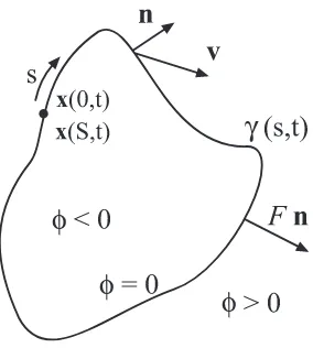
Consider a boundary a curve in two dimensions or a surface in three dimension -separating one region from another. The motion of this boundary is defined by a known speed functionF in a direction normal to itself, where the normal direction is oriented outward with respect to a pre-defined inside and outside. The boundary does not necessarily have to be a closed boundary as long as the orientation of the speedF with respect to the two possible normal directions has been defined. The goal is to track the motion of the interface as it evolves. Only the motion of the interface in its normal direction is considered; motions in the tangential directions are ignored. The speed function can depend on many factors including the position of the boundary, its curvature and normal direction.

Given a simple, smooth, closed initial curve γ in R2 _{and the family of curves} γ(t) generated by moving γ along its normal vector field with speed F, a natural approach is to parameterize γ at time t using the position vector x(s, t), where

s is the path length along the interface (see figure 2.1). The total length of the front is given by S with 0 _≤ s _≤ S which means that x(0, t) = x(S, t). This is a Lagrangian formulation because x(s, t) describes the moving front explicitly.

Under the assumption thatF > 0 the front always moves outward. An alter-native way to characterise the position of this expanding front is to calculate the arrival time T(x) of the front as it crosses each point of an underlying grid. The equation for this arrival time function T(x) is then given by

where Γ is the initial position of the interface and _∇T is the gradient of the arrival time field orthogonal to the front. The motion of the front is now described by the solution to a boundary value problem, which is an Eulerian formulation because the front is given by the contour line of the arrival time field which has been defined on a grid. This boundary value formulation eventually gives rise to the fast marching method. If the speedF depends only on the position (i.e.F =F(x)) then (2.1) reduces to what is known as the eikonal equation in seismology.

The eikonal equation is the so-called high frequency approximation of the full elastic wave equation (e.g. Aki & Richards, 2002). It is derived from the elastic wave equation under the assumption that the wavelength of the propagating wave is substantially shorter than the seismic heterogeneities it encounters (e.g. ˇCerven´y, 2001; Chapman, 2004). It is normally given as (Chapman, 2004)

|∇T_|=s (2.2)

where s = 1/F is slowness and T is a time function (the eikonal) which describes surfaces of constant phase (wavefronts) when T is constant.

However, if the speedF is permitted to vary in sign the front can move forward or backward and hence may pass over a point x of the underlying grid several times. In this case the crossing time or arrival time T(x) is no longer a single valued function. One way of accounting for this added complexity is to define the initial position of the front as the zero level set (zero contour line) of a higher dimensional function φ (i.e. a signed distance function). The evolution of this function φ can then be linked to the propagation of the interface through a time dependent initial value problem where the position for a given time corresponds to the zero level set of φ. This initial value formulation eventually leads to the level set method.

2.2

Level set method

2.2.1

Level set equation

The aim now is to derive an equation of motion for the level set function φ by matching the zero level set of φ with the evolving front. The level set value of a particle x(t) moving along with the front must always be zero, and therefore

φ(x(t), t) = 0. (2.3)

The time derivative of (2.3) is found with the chain rule

φt+∇φ(x(t), t)·xt(t) = 0, (2.4)

where φt and xt(t) denote derivatives with respect to time. Since the scalar speed

function F is defined as the speed in the outward normal direction, one can write

F =xt(t)·n, (2.5)

where n is the unit normal vector to the interface defined by

n= ∇φ

|∇φ_|. (2.6)

Substituting (2.6) into (2.5) yieldsF_|∇φ_|=_∇φ_·xt(t) and from (2.4) the evolution

equation for the signed distance function φ is:

φt+F|∇φ|= 0, given φ(x, t= 0). (2.7)

This is the level set equation formulated by Osher & Sethian (1988), and cor-responds to equations describing advective transport in an incompressible fluid. From a conservation law point of view (2.7) states that for a given point the change of a property with time (for example the concentration of a substance in a fluid) is equal to the flux of this property in the direction of the gradient. If the speed function F depends on the curvature of the interface, i.e. on the second derivative of the signed distance function, the level set equation becomes what is known as a hyperbolic conservation law.

velocity v(x), which is a vector field. The level set equation (2.7) then becomes

φt+v· ∇φ= 0, given φ(x, t= 0). (2.8)

The velocity v in (2.8) or the speed F in (2.7) may depend on many factors. For example, F can depend on local geometrical information associated with front curvature, or the direction of the local wavefront normal. In fluid dynamics it is common to encounter an interface evolving under curvature dependent motion (e.g. Osher & Sethian, 1988; Evans & Spruck, 1991). Examples of local properties influencing the evolution of an interface are bubble dynamics and two phase flow where surface tension plays a role (e.g. Sussman et al., 1994; Chang et al., 1996).

F can also be influenced by the global properties of a front (i.e. its shape and position), and might depend on integrals along the front and/or associated differ-ential equations. A particular example of this occurs when an interface is a source of heat that affects diffusion on either side of the interface which, in turn, affects the motion of the interface (e.g. Ruuth, 1998). In seismic wavefront tracking, the speed of the front is a function of position x, and does not depend on the shape of the front. It is also possible to define a speed which depends on more than one of these properties, for example, a gas bubble rising in a moving fluid.

2.2.2

Signed distance function

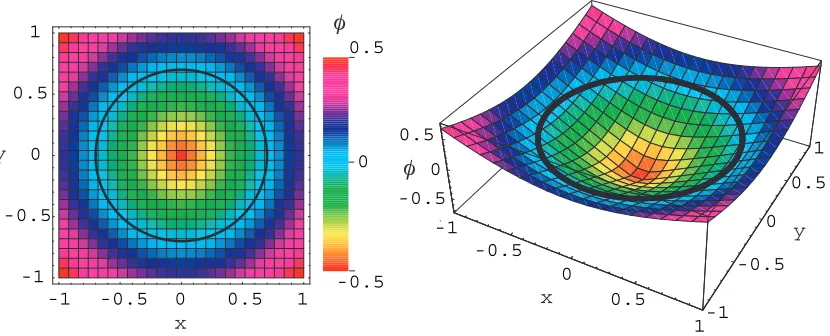
A natural choice for the implicit representation of a curve in two dimensions or a surface in three dimensions is a signed distance function. For each node of the underlying grid, the distance to the closest point on the curve or surface is calculated. The distance is negative for points inside of the front and positive for points outside of the front (see figure 2.2 for an example in two dimensions).

Such a signed distance function φ is well behaved when the absolute value of the gradient is equal to one for every point in the computational domain. In this situation (2.7) reduces to φt = −F and the values of φ either increase or

decrease, depending on the sign of F. When F > 0 the interface moves in the outward normal direction, and when F < 0 the interface moves in the inward normal direction. When F = 0 the equation reduces to φt = 0 and hence the

interface does not move.

-1 -0.5 0 0.5 1 -1

-0.5 0 0.5

1

0.5

-0.5

-1 -0.5

0

0.5 1

x

-1 -0.5

0 0.5

1

y

-0.5 0 0.5

φ

-x

y ₀

φ

Figure 2.2: Signed distance functionφused to implicitly define a circle with radius 0.75 and centre (0,0).

distance function has to exhibit a reasonable behaviour at the occasional kinks where _|∇φ_| is not defined.

The concept of a signed distance function requires that there is an inside and outside with respect to the interface. If the interfaces have multiple junctions, for example a network of soap bubbles or grain boundaries in a rock, the idea is to assign to each region (i.e. individual soap bubbles or grains) a separate signed distance function to describe its boundary (e.g. Merriman et al., 1994; Zhao et al., 1996b). The signed distance functions are then evolved independently, which means that gaps between the regions (i.e. soap bubbles or grains) are likely to develop. In a so called interaction step, the signed distance functions assigned to the different regions can be updated so that the junction points (i.e. where boundaries meet) show the desired behaviour (Merriman et al., 1994).

2.2.3

Basic algorithm for interface evolution

0 0.5 1 1.5 2 2.5 3 3.5 4

-4 -3 -2 -1 0 1 2 3 4

time t

distance x

A

B

Figure 2.3: Characteristic curves (red lines) for F = 1 in the x-t plane. u is constant along lines with slope 1.

2.2.3.1 Solution in one dimensional space

Consider the level set equation for a one dimensional problem, where the signed distance function is given by u:

ut(x, t) +F ux(x, t) = 0 with u(x,0) =f(x), (2.9)

where ut is the time derivative of u, ux the spatial derivative and F the speed.

Although it still can be viewed as a conservation law, (2.9) is also the one dimen-sional wave equation, and for constantF a solution is given byu(x, t) = f(x₋F t). This means that the solution u at any point x at time t is given by the value of the initial data at the point x₋F t on the x axis. In addition, the solution u

is constant along lines of slope F in the x-t plane (figure 2.3). Considering two points A and B in the x-t plane the solution at point A can be found by tracing back along a line with slope F to the point B on the x-axis. Hence, in formal terms, the domain of dependence of the point A is the point B. Conversely, the set of points on the line with slope F emanating from point B is referred to as the domain of influence of point B. The lines of constant uin the x-t plane are known as characteristics, and more specifically, those in figure 2.3 are the characteristics of the one dimensional wave equation (2.9) with F = 1.

x

t

∆

t

∆

x

(i,n)

time

distance

Figure 2.4: Computational grid used to solve (2.9).

a time step of ∆t (figure 2.4). Every grid point can then be represented by a coordinate pair (i, n) corresponding to the point (i∆x, n∆t). The time derivative

ut in (2.9) can be approximated by a forward finite difference operator,

ut=

un_i+1₋un i

∆t . (2.10)

Substituting the forward finite difference operator (2.10) for ut in (2.9) produces

the following expression for un_i+1,

un_t+1=un_{t −}∆tuxF, (2.11)

which can be used to approximate u ahead in time once the spatial derivative

ux is calculated. The spatial derivative can be discretised using a forward ∆+ux,

backward ∆−_u

x or centred ∆0ux finite difference operator. These operators are

given as

∆+ux = un

i+1−uni

∆x , (2.12)

∆−_u

x =

un

i −uni−1

∆x , (2.13)

∆0ux = un

i+1−uni−1

2∆x . (2.14)

0 0.5 1 1.5 2 2.5 3 3.5 4

-4 -3 -2 -1 0 1 2 3 4

time t

distance x

Figure 2.5: Characteristics of the one dimensional wave equation where F is a function of x and tgiven by F(x, t) =₋2₅x(t+1₄).

The backward scheme (2.13) in this situation is referred to as an upwind scheme because it uses values upwind of the direction of information propagation, which is clearly preferable, as it sends information in the direction that correctly matches the differential equation. Generally speaking, the numerical domain of dependence should contain the mathematical domain of dependence. One commonly refers to the set of nodes used for the computation of a spatial derivative at a certain node as a stencil.

IfF is function ofxand/ort, the characteristics are no longer given by a set of parallel straight lines (see figure 2.5). Instead lines may converge and form what is known as a shock in fluid dynamics, or diverge and form what is known as a rarefaction. Hence, which finite difference operator is chosen for the approximation of ux at the nodes along xfor a given time t, will depend on the local direction of

information flow, so that the numerical domain of dependence always includes the mathematical domain of dependence.

F(x1) > 0 F(x2) < 0

x1 x2

F(x1) < 0 F(x2) > 0

x1 x2

F(x1) < 0 F(x2) < 0

x1 x2

F(x1) > 0 F(x2) > 0

x1 x2

to the left to the right shock rarefaction

Figure 2.6: Possible configurations of characteristics around a point in thex-tplane.

Figure 2.6 shows all possible cases for the directions in which information is sent from a node of the computational grid at a given time.

1. F(x1), F(x2)<0: The wave moves to the left and information is sent from right to left. Therefore the forward finite difference operator should be used. 2. F(x1), F(x2)>0: The wave moves to the right and information is sent from left to right. Therefore the backward finite difference operator should be used.

3. F(x1)>0, F(x2)<0: Two waves collide and a shock develops, which moves with the sum of the two speeds, since the speed on the right is negative (the characteristics move to the left) and speed on the left is positive (character-istics move to the right).

4. F(x1)< 0, F(x2)> 0: The wave is split in two and a rarefaction develops, which does not move, since the speed on the right side is positive (character-istics go to the right), while the speed on the left is negative (character(character-istics move to the left).

One can then directly write down a finite difference scheme for ux, which chooses

the correct operator for all four cases:

ux =

p

max(∆−_u

x,0)2 + min(∆+ux,0)2 (2.15)

The resulting scheme for updating a discretised signed distance function in R1 _is

then given as

un_i+1 =un_{i −}∆tpmax(∆−_u

x,0)2+ min(∆+ux,0)2, (2.16)

with ∆−_u

x and ∆+ux given by (2.12) and (2.13) respectively. This solution of a

as a viscous solution or minimum entropy solution; by taking the flow of infor-mation into account the numerical scheme stays well behaved. In the following section the scheme will be extended to higher spatial dimensions.

2.2.3.2 Solution in a higher dimensional space

The level set equation (2.7) for three spatial dimensions can be written in the form of the general Hamilton-Jacobi equation

φt+H(φx, φy, φz, x, y, z) = 0, (2.17)

where H is known as the Hamiltonian, which for the level set equation (2.7) is given by

H(φx, φy, φz, x, y, z) =F

q

φ2

x+φ2y +φ2z. (2.18)

A one dimensional version of (2.17) can be written

φt+H(φx) = 0. (2.19)

Partial differentiation of (2.19) with respect to x reveals

∂φx

∂t + [H(φx)]x = 0. (2.20)

Substituting u=φx gives the hyperbolic conservation law

ut+ [H(u)]x= 0. (2.21)

This means that the viscous solution of the level set equation, as introduced in the previous section, can also be computed using schemes proposed for general Hamilton-Jacobi equations (Sethian, 1999). This link is useful, because there exists a wide variety of higher order numerical solvers for general Hamilton-Jacobi equations, which are known to converge to the viscous solution (e.g. Osher & Sethian, 1988; Jiang & Peng, 2000; Zhang & Shu, 2003; Bryson & Levy, 2003), and therefore can be used here.

for higher dimensional Hamilton-Jacobi equations for symmetric Hamiltonians can be built by simply replicating each spatial variable. This allows a finite difference scheme for the level set equation to be built for any given m dimensional space. By applying (2.16), a scheme for three spatial dimensions is given by (Osher & Sethian, 1988)

φn_i,j,k+1 =φn_{i,j,k −}∆t[max(Fi,j,k,0)∇++ min(Fi,j,k,0)∇−], (2.22)

where

∇+= [ max(∆−_φ

x,0)2 + min(∆+φx,0)2+

max(∆−_φ

y,0)2+ min(∆+φy,0)2+

max(∆−φz,0)2+ min(∆+φz,0)2]

1

2 (2.23)

and

∇−_{= [ max(∆}+_φ

x,0)2+ min(∆−φx,0)2+

max(∆+φy,0)2+ min(∆−φy,0)2+

max(∆+φz,0)2 + min(∆−φz,0)2]

1

2. (2.24)

∆−_φ

x, ∆−φy and ∆−φz are the first order backward finite difference operators in

thex,yandz direction, and ∆+_φ

x, ∆+φy and ∆+φz are the corresponding forward

first order finite difference operators. If the interface moves under the influence of a velocity v (see (2.8)) instead of the speed F in the outward normal direction (see (2.7)), the scheme for three spatial dimensions is as follows:

φn_i,j,k+1 =φn_i,j,k−∆t

[ max(vx_i,j,k,0)∆−_φ

x+ min(vi,j,kx ,0)∆+φx

max(vy_i,j,k,0)∆−_φ

y + min(vyi,j,k,0)∆ +_φ

y

max(vz_i,j,k,0)∆−φz+ min(vzi,j,k,0)∆+φz], (2.25)

where vx i,j,k, v

y

i,j,k and vzi,j,k are thex, y and z components of the velocity vector v

at the point (i, j, k).

0 2 4 6 8 10

y

0 2 4 6 8 10 12 14

x

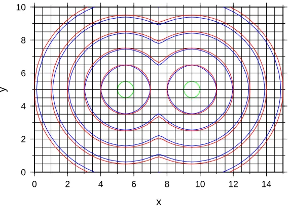
Figure 2.7: Two interfaces start off as a circles (green lines) and propagate with a constant speed of one in their outward normal direction. They merge and form one new interface. The interfaces are calculated using a first order accurate scheme (blue lines) and a fifth order WENO scheme (red lines) and plotted at 1 s intervals; interface segments parallel to the grid lines should therefore coincide with them.

dimensions or a surface in three dimensions. The first order scheme (2.22) will now be used to describe the evolution of an interface in two spatial dimensions. This means that derivatives with respect toz and the corresponding discretisation

k are simply omitted in (2.22), (2.23) and (2.24).

In figure 2.7 two interfaces begin as circles of radius 0.5 (shown in green). The grid for the signed distance function consists of 50_×75 nodes and the time step is 0.125 s. The speedF is defined in the outward normal direction and is equal to one. The interfaces are extracted after having up-sampled the signed distance functions using a cubic B-spline approximation. Due to the extraction of the zero level set contours at 1 s intervals, interface segments parallel to the grid lines in figure 2.7 should coincide with them. The interfaces computed using the first order method previously introduced are plotted in blue, while the red interfaces were computed using a higher order solver which will be introduced in the next section. Clearly the higher order approximation is preferable.

0 2 4 6 8 10

y

0 2 4 6 8 10 12 14

x

0 1 2 3 4

φ

Figure 2.8: Signed distance function for one time step of the merging circle example. The line along which the signed distance function is discontinuous is indicated by the black arrows. The interface is given by the black line. The discontinuity has been preserved by using a fifth order WENO scheme for the approximation of the spatial derivatives.

of the evolving boundary are handled naturally. This explains why the level set method has been widely used in the field of fluid dynamics (e.g. Mulder et al., 1992; Sussman et al., 1994; Chang et al., 1996).

It is worthwhile remembering at this stage that a seismic wavefront becomes self-intersecting as it develops a swallowtail pattern in the presence of a low veloc-ity anomaly (figure 1.1). Hence the level set method cannot be used directly to describe the wavefront. It will be shown later that it still can be used for wavefront tracking based on the concept of reduced phase space (see section 2.3), which al-lows the unfolding of a wavefront so that it no longer self-intersects (Osher et al., 2002). For the moment, however, the focus will be on further investigation of the level set method.

2.2.3.3 Higher order finite difference operator

x

x

centred finite difference operator

smoothest stencil

a) b)

Figure 2.9: The gradient of a signed distance function is computed for a node (filled circle) near a discontinuity using two different finite difference operators. The two dif-ferent gradients are plotted in the black boxes. (a) The stencil uses nodes on both sides. (b) The stencil is based on the smoothest set of nodes. Clearly only the scheme used in (b) can recover the correct gradient (red line).

tend to smooth out discontinuities in the signed distance function if their stencil includes a discontinuity like the one shown in figure 2.8. Here, a discontinuity in the signed distance function is visible along the line, indicated by the black arrows, along which the circles are merging. If it is important to represent this merging accurately, one has to avoid a smearing out of the discontinuity of the signed distance function.

The ideal approach is to use higher order accurate schemes designed for piece-wise smooth functions containing isolated discontinuities. ENO (essentially non oscillatory) and WENO (weighted essentially non oscillatory schemes) are such schemes, and have been developed with hyperbolic conservation laws and related Hamilton-Jacobi equations in mind. ENO schemes were first proposed by Harten et al. (1987). Their idea was to start with one or two nodes and then add one node at a time to the stencil from the two neighbour candidates to the left and right. The node which provides the smoother stencil is then chosen to be added to the stencil.

on the left side of the discontinuity are used) the correct gradient is computed (figure 2.9b).

In figure 2.8, the grid resolution used for the signed distance function is too coarse to reproduce the sharp corner where the circles merge. Up sampling the signed distance functions using a spline before the interface is extracted helps to reveal the sharp corners (see figure 2.7) one would expect for two merging circles. ENO schemes based on point values and TVD (total variation diminishing) Runge Kutta time discretisations for multiple space dimensions have been intro-duced by Shu & Osher (1988, 1989). In these schemes, the smoothest stencil is chosen at each node from a set of stencils which could be used to approximate the finite difference operator. Jiang & Shu (1996) and Liu et al. (1994) introduced weighted ENO (WENO) schemes as an improvement over the ENO schemes. They use a convex combination of all candidate stencils instead of just one as in the orig-inal ENO scheme.

The higher order approximation of the level set equation used in this work is based on a fifth order WENO discretisation in space together with a third order TVD Runge Kutta discretisation in time. This discretisation has previously been suggested by Jiang & Peng (2000). In general, there are many acceptable solvers for Hamilton-Jacobi equations that could be used to approximate the level set equation. One should also keep in mind that the field of solving hyperbolic conser-vation laws (e.g. Jiang & Tadmor, 1998; Ammar et al., 2006) and Hamilton-Jacobi equations (e.g. Serna & Qian, 2006; Lin & Liu, 2007) is vast and new techniques are continually under development. Comprehensive discussions of earlier work in the field of hyperbolic conservation laws have been given by LeVeque (1992) and Sod (1985).

In the scheme used here, which is based on a regular grid, space and time is discretised into a collection of grid points with a spatial spacing of ∆x and ∆y

and a time step ∆t. Every grid point is represented by a coordinate triplet (i, j, n) corresponding to the point (i∆x, j∆y, n∆t). The value of the signed distance function φ at the node (i, j) of the grid at time n∆t is given by φn

i,j. The spatial

derivatives are discretised using a fifth order WENO scheme in space. The forward ∆+ _{and backward ∆}− _{finite difference approximations for the first derivative of} the signed distance function in the xdirection at the grid node (i, j) are given by

∆±_φ

x,i,j = ±

(φi±1,j−φi,j)

The finite difference approximation to the second derivative in the x direction at the grid node (i, j) is given by

∆−∆+φx,i,j =

φi−1,j−2φi,j+φi+1,j

∆x2 . (2.27)

Analogously one can define the finite difference operators in the y direction.

WENO schemes are basically centred schemes in regions where the solution is smooth. If there is a discontinuity inside the stencil, the WENO scheme can effectively choose the smoothest sub stencil for the approximation and therefore avoid undesirable oscillations (Jiang & Shu, 1996). The backward (left) finite difference in the x direction is given by the following fifth order WENO scheme (Jiang & Peng, 2000)

∆−

W EN Oφx =

1 12(−∆

+_φ

x,i−2,j+ 7∆+φx,i−1,j+ 7∆+φx,i,j −∆+φx,i+1,j)−∆xΦW EN O(∆−∆+φx,i−2,j,

∆−∆+φx,i−1,j,∆−∆+φx,i,j∆−∆+φx,i+1,j), (2.28)

where

ΦW EN O(a, b, c, d) = 1

3ω0(a−2b+c) + 1 6(ω2−

1

2)(b−2c+d) (2.29) with weights defined as

ω0 =

α0 α0+α1+α2

, ω2 =

α2 α0+α1+α2

,

α0 =

1 (ǫ+β0)2

, α1 =

6 (ǫ+β1)2

, α2 =

3 (ǫ+β2)2

;

β0 = 13(a−b)2+ 3(a−3b)2, β1 = 13(b−c)2+ 3(b+c)2, β2 = 13(c−d)2+ 3(3c−d)2.

Here ǫ is used to prevent the denominators from becoming zero. The solution is relatively insensitive to the values chosen for ǫ. Jiang & Peng (2000) useǫ= 10−6

forward (right) finite difference in the x direction is given by

∆+_{W EN O}φx =

1 12(−∆

+_φ

x,i−2,j+ 7∆+φx,i−1,j+ 7∆+φx,i,j −∆+φx,i+1,j)−∆xΦW EN O(∆−∆+φx,i+2,j,

∆−_∆+_φ

x,i+1,j,∆−∆+φx,i,j,∆−∆+φx,i−1,j). (2.30)

By replacing the x direction with the y direction, expressions for ∆−

W EN Oφy and

∆+_{W EN O}φy can be written. One can then replace the first order finite difference

operators (e.g. ∆+_φ

x) for the spatial derivatives in (2.23) and (2.24) with the

corresponding fifth order WENO finite difference operator (e.g. ∆+_{W EN O}) so that (2.22) becomes a scheme with fifth order accuracy in space.

So far the focus has been on the spatial discretisation. It is important to note that near discontinuities, the fifth order WENO scheme essentially steps back to a third order ENO scheme so that the finite difference operator is based on the smoothest stencil. Hence a third order accurate finite difference operator in time is sufficient to match the spatial WENO scheme. Here, the third order TVD Runge Kutta scheme given by Shu & Osher (1988) and Gottlieb & Shu (1998) is used. Thus, the finite difference approximation to the level set equation becomes

φ1_i,j =φn_i,j−∆t[max(Fi,j,0)∇+,min(Fi,j,0)∇−], (2.31) φ2_i,j = 3

4φ n i,j + 1 4φ 1

i,j−∆t[max(Fi,j,0)∇+,min(Fi,j,0)∇−], (2.32) φn_i,j+1 = 1

3φ n i,j + 2 3φ 2 i,j− 2

3∆t[max(Fi,j,0)∇

+_,min(F

i,j,0)∇−]. (2.33)

2.2.3.4 Numerical realisation

and the speed F given by

max(F)∆t_≤∆x, (2.34)

where the maximum is taken over all values of F at all possible points within the domain, not simply those corresponding to the zero level set. Due to the CFL condition, increasing the grid resolution by a factor of two means that one must halve the time step.

The value ofF must be known at all grid nodes of the signed distance function. This poses no problem if the speed is given by an analytical function. On the other hand, if the speed is only known on a coarser grid, then some form of interpolation has to be applied. In the following, a cubic B-spline approximation is used for the speed F. If F is given on a regular grid as ci,j its value at an arbitrary position

(u, v) in the grid cell (i, j) is given by

Bi,j(u, v) = 2

X

l=−1 2

X

m=−1

blbmci+l,j+m, (2.35)

where u(0 _≤ u _≤ 1) and v(0 _≤ v _≤ 1) are expressed as a fraction of the grid spacing. The weighting factors bl, bm are the uniform cubic B-spline functions

(Bartels et al., 1987). When approximating the level set equation having a smooth speed function F is an advantage from a stability point of view. A cubic B-spline approximation has the property that the resulting field has continuous first and second derivatives (see appendix B), yet is locally controlled.

The computational domain is finite, so the finite difference stencils used to ap-proximate the spatial derivatives may extend outside of the computational domain when working near a boundary. This means that ghost nodes have to be added to the computational grid. Two types of boundary conditions are used.

1. Periodic boundary conditions: For each dimension, values from one end of the grid are copied across the grid to the ghost nodes at the other end of the grid and vice versa.

2. Extrapolating boundary conditions. The values of the signed distance func-tions are for each dimension linearly extrapolated away from zero into the ghost nodes.

the existence of a ghost interface, as the value of the signed distance function cannot become 0 for a ghost node.

Using all the concepts introduced so far, it is now possible to propagate an interface by updating the signed distance function for the whole computational domain. This is the so-called global level set method (e.g. Sethian, 1999; Osher & Fedkiw, 2003). However such an approach has two disadvantages. Firstly, only a few nodes of the underlying grid are actually near the interface and are essential to describing its position. Nodes distant from the zero level set still get updated but they tend to have little to no influence on the zero level set. Hence it can be inefficient to update all nodes of the underlying grid for each time step. Secondly, despite the stability preserving finite difference solvers, a signed distance function might develop kinks and could become very flat (_|∇φ < 1_|) or steep (_|∇φ > 1_|) near the interface. It therefore would be desirable to regularise the signed distance function from time to time so that the value of the gradient of the signed distance function is again equal to one for most nodes.

2.2.4

Improved algorithms for interface propagation

A global level set method can be improved using the following concepts:

• Reinitialisation: During the propagation process a signed distance function may become less well behaved i.e._|∇φ_{| 6}= 1. As this influences the accuracy of the scheme a reinitialisation of the signed distance function can be performed so that it is again well behaved for most of the grid nodes i.e._|∇φ_|= 1. This will generally increase the accuracy, especially for complex interface motion.

• Narrow band: In general only the zero level set of the signed distance function is of interest. One way of increasing the efficiency of the method involves updating the signed distance function in a narrow band around the zero level set. As the interface moves, the narrow band must be moved with it.

0 2 4 6 8 10

y

0 2 4 6 8 10

x

0 2 4 6 8 10

y

0 2 4 6 8 10

x

0.0 0.5 1.0 1.5

|∇φ|

a) b)

Figure 2.10: A circle (green line) has been expanded with a speed F in its outward normal direction given by F(x, y) = 1.0/(1.0 + exp(₋(y₋5.0)2). (a) Gradient of the signed distance function and zero level set (black line) with no reintialisation. (b) Same as (a) except now with reintialisation after each time step.

presented by Berger & Colella (1989) for solving hyperbolic conservation laws in two dimensions.

Recent implementations of the level set method tend to combine all three con-cepts (e.g. Losasso et al., 2006). Here, however, the focus will be on a narrow band level set method which requires that the signed distance function can be reinitialised at any given node. Hence, the concept of reinitialisation is introduced first.

2.2.4.1 Reinitialisation

For numerical accuracy the signed distance function has to be well behaved for most nodes of the grid. This means that except for isolated grid nodes the value of its gradient should be equal to one i.e.

|∇φ_|= 1. (2.36)

In figure 2.10a, a circle has been expanded in its local normal direction with a speed given by F(x, y) = 1.0/(1.0 + exp(₋(y₋5.0)2_{). Instead of the value of}

the signed distance function, the value of its gradient is plotted. Clearly, it is no longer equal to one near the interface. Therefore a procedure is needed to reset φ