in Tree Growth Prediction and Planning
A thesis submitted in fulfilment of the requirements for the degree of Doctor of Philosophy (Forestry).
Oliver Chikumbo
Department of Forestry
Australian National University Canberra, ACT 0200, Australia
But many of the priests and Levites and chief of the fathers, who were ancient men, that had seen the first house, when the foundation of this house was laid before their eyes, wept with a loud voice; and many shouted aloud for joy:
Ezra 3:12, -Holy Bible (KJV)
I
I I
I
1,'
I
_
,
,
,,II
1: 11
I, ' I
'
Except where otherwise indicated this thesis is
my
own work.I
Oliver Chikumbo
IV
Acknowledgments
Many thanks to my mum Regina Chikumbo and brother-in-law, Steve Moyo for their overwhelming support at the start of my research program. I am also grateful to my supervisors, Dr. Brian Turner and Dr. I.M.Y. Mareels, who had ample time to listen and to give me exceptionally constructive advice and a myriad of references to read. This helped me to clearly define my research problem.
Acquiring data proved to be a major problem and through Dr. Ryde James (Department of Forestry, Australian National University), I managed to secure data from the Forest Research Institute and Tasman Forestry (New Zealand) and I am really grateful to him. Many thanks to Stuart Christie (Forestek-CSIR, South Africa), who made it possible for me to work with Heyns Kotze (Forestek-CSIR, South Africa), which proved to be one of my most rewarding time in my research career. Through Forestek I secured data to fully authenticate system identification and optimal stand density control.
I am also grateful to the Department of Natural Resources and Environment (DNRE) and especially to Fiona Hamilton and Bruce Kilgour who managed to secure a job for me, so that I could complete my research. I am now
employed on a full-time basis as a Forest Biometrician for DNRE. I am also thankful to my friends, James Allnutt, James and Karen Nachipo, Deb O'Connell, Carol and Martin Mutendeudzi and Florence Soriano who stuck to me like family during my research. Many thanks to Roland Jahnke (Department of Forestry, Australian National University) for assisting me to acquire MatLab from Ceanet (Sydney).
Determining optimal thinning strategies on a stand basis for forest
plantations is a problem that forest analysts have solved with multi-stage
optimisation procedures based on dynamic programming ideas. Recent literature
suggests that the Principle of Optimality is violated by the forestry formulations of
dynamic programming - this is the neighbourhood storage concept that limits
exhaustive search of a solution at each decision stage, followed by a forward recursive
optimisation. This particular formulation has been largely driven by an attempt to
overcome the 'curse of dimensionality' forced on by computer memory limitations.
Another problem which confronts the analyst is the absence of suitable forest growth
models (ones directly related to the decision variable).
In this thesis, models based on control theory are used successfully to solve the optimal thinning strategy problem. These models are nonlinear dynamical
(input/ output) models (Systems Engineering terminology used to describe dynamic
systems, where control and controlled variables are identified). To fully account for the nonlinearities in the observed growth trends, a 2-stage modelling approach is adopted; in the first stage a linear dynamical model, acounting for the general growth trend, is identified and in the second stage the parameters from the model in the first stage are modelled as functions of initial densities, thus resulting in a nonlinear
dynamical model with good predictive properties; the growth dynamical models
developed for Pinus patula stands were significantly better in prediction than previously published growth models.
A state space control model is developed (from these dynamical models)
II
I
i
11 I
I I I I
I
Vl
vector of the number of standing trees (stems/ha)), stand basal area (m2 /ha) and
mean stand height (m)) represents sufficient growth information to predict the future
output; and the output (expressed as stand volume in m3 /ha) represents the growth
response.
In addition to this control model a cost functional is formulated to
maximise volume or value production over a specified rotation length. A control
sequence is then determined by using an iterative solution technique such as dynamic
programming or the maximum principle.
The silvicultural strategies determined from the control model were
comparable with those determined from long-term analysis of trial experimental data;
an indication of the reliability of the control model. In the event of changes in market
forces, political emphasis, climate or site productivity, the control model can be
reliably used to promptly determine alternative strategies by manipulating the
constraints and/ or the cost functional.
Growth data from Australia (Victorian Department of Natural Resources
and Environment), New Zealand (Forest Research Institute and Tasman Forestry) and
South Africa (Forestek-CSIR) were used. The data were from three types of forests
namely the Eucalyptus mixed-species forests (Victoria, Australia), Pinus radiata
plantation forests (New Zealand) and Pinus patula plantation forests (South Africa).
MatLab software is used for developing dynamical models and a
FORTRAN program called DMISER3, is used to find solutions to the optimal control
formulations.
CHAPTER 1
Introduction
1.1 Recent 'forestry dynamic programming' formulations
1.2 Aims
1.3 Theme and chapter outline
CHAPTER2
System Identification
2.1 System Identification
2.1.1 Dynamical Systems
2.1.2 System Identification procedure
2.2 The Linear Model Description
2.3 Modelling for Simulation, Prediction and Control
2.3.1 Simulation
2.3.2 Prediction
2.3.3 Control-Optimal
2.4 Arguments for dynamical models
2.5 Modelling Software: MatLab
2.5.1 MatLab Software
Endnote 2A: Detrending and Stabilisation of Variance
CHAPTER3
Models of Linear Time-Invariant Systems
3.1 Model Structures
3.2 Black-box models
3.3 State -Space Models
1 4
7
8
9
10
11
13
16
19
19
2021
24 31
33
35
38
39
40
Endnote 3A: AR process Endnote 3B: MA process
Endnote 3C: First- and second-order systems
CHAPTER4
Vlll 49 54 56
Dynamical Models for Plantation Forests 59
4.1 Introduction 59
4.2 Objective 59
4.3 Dataset 60
4.4 Method 63
4.4.1 Growth model types 65
4.4.2 Model development 66
4.5 Diameter Growth Modelling 69
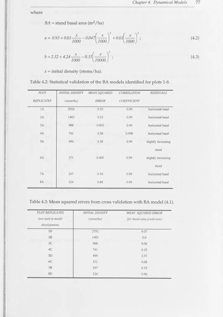
4.6 Model Structure Selection and Model Validation 73
4.6.1 Mortality function 75
4.6.2 Basal area function 76
4.6.3 Thinning responses 82
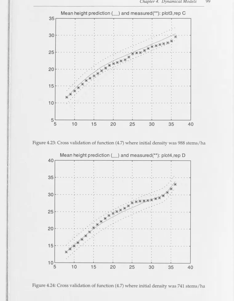
4.6.4 Average height function 93
4.6.5 Volume function 102
Appendix 4A: Correlation functions calculated within 99% confidence limits for
the cross validation plots and the BA model, (4.1). 109
Appendix 4B: Correlation functions calculated within 99% confidence limits for
the cross validation plots and the height model (4.5) 114
CHAPTERS
Plantation Performance Modelling 5.1 Introduction
5.2 Optimal Control
5.2.1 Optimum Management Strategies
5.4 Comparison of DMISER3 regimes and current South African P. patula regimes131
5.5 Prediction and Partitioning of Yield 136
5.6 Conclusion
Appendix SA: A typical DMISER3 output for a volume production stand regime
with a rotation age of 25 years and an initial planting density of 2000 stems/ha,
138
where 0 < u(t) < 1000, 'tit E [t, TJ. 140
CHAPTER6
Recursive Identification for Forest Dynamical Models
6.1 Mean dominant height
6.2 Recursive identification
6.3 Forestry example of recursive identification: development of a generic yield
curve
CHAPTER 7
Extensions
7.1 Hydrological applications
7.2 Economic improvements
7.3 Speculative applications
CHAPTERS
Conclusion
REFERENCES
142
142
146
148
154
154
154
157
159
APPENDIX I
Choosing a Model Class
1.1 Building Simple Models from Process Data
1.2 Comparison between different identification methods
1.3 Model structure determination
1.4 State space models
Endnote IA: Pole-zero plots
APPENDIX II
Optimal Control
II. l Historical Account
II.2 Control concepts for discrete-time systems
II.2.1 Stability
II.2.2 Controllability and Reachability
II.2.3 Observability
II.3 Multistage decision processes
II.4 Dynamic programming
11.5 Discrete maximum principle
II.6 General remarks on the MP and DP
II.7 Optimal design method: state space approach
II.7.1 Linear Quadratic Control
X
II.8 DP in the determination of Optimal Stand Density for Intensively managed
181
183
192
202
207
210
212
212
215
215
216
219
221
224
226
228
230
234
Plantation Forests 236
Endnote IIA: A typical example of a forestry DP formulation for a thinning
-I '
11
'
10
II
i
I
I
I I 'APPENDIX III
DMISER3: Information for the user 242
DMISER3 input data file 245
A MatLab constrained optimisation program for South African Pinus patula 265
I'
INDEX FOR KEYWORDS 270
CHAPTER 1
Introduction
Planning is the problem of determining an optimal procedure for attaining
a set of objectives (Luenberger, 1969). In timber production, planning has been
primarily concerned with 'forest regulation' based on the desirability of attaining some
'target forest' structure (Clutter, et al., 1983). Forest regulation was a harvesting
control that was determined from timber inventories conducted to find out the total
volume in a forest. This information was used in models to calculate a sustainable
yield for the forest, based on average forest-wide growth rates (Turner, 1995). Each
year the sustainable yield had to be removed from the forest after a thorough check of
maps to determine where the cut could be taken from. Usually this was done only for
the first few years; rarely was a check done to see whether at the end of the cutting
cycle or rotation it would be possible to begin again (Turner, 1995).
However, the objectives have changed in recent years and are more
concerned with immediate, rather than distant future, characteristics of the forest.
Planning the management of a plantation forest, which is the focus of this thesis, now
consists of defining operational area units and estimating the growth and yield for
each unit under a set of alternative activities (harvesting/ silvicultural practices).
Planning is the most important level of control in any forest enterprise because it is
primarily through planning that a high level manager exerts influence over his or her
organisation. Accurate estimations of growth and yield provide a basis for
determining the 'best' options for maximising management objectives; computer
decision support systems built from growth and yield models are used to evaluate the
different forest management options for bare land or existing forest stands. These
options are ranked in terms of volume or value production criteria and optimum
planting densities, thinning1 regimes or rotation ages can be determined.
1
The growth and yield models describe different components of plantation
growth and may include models for dominant height growth, survival, basal area
growth, volume growth, diameter distribution and height by diameter class (Harrison,
et al., 1994). A forest planning decision support system may incorporate a
mathematical programming formulation because a choice has to be made between
alternative options. Optimisation techniques have been and are still being used to
determine a schedule of activities to satisfy management objectives. An important
subclass of mathematical programming formulations is dynamic programming.
Problems which require sequential decision-making in forest planning ( or
any other discipline) can be dealt with effectively if considered in a multi-stage
optimisation framework. In a multi-stage optimisation formulation the outcomes at
each and every stage are calculated on the basis of the Principle of Optimality
(Bellman, 1957) that basically states that whatever the first decision is for an optimal
policy, the remaining decisions must constitute a policy with regard to the state
resulting from the first decision.
Various tools are available to find solutions to multi-stage optimisation
problems. Dynamic programming and maximum principle are the two solution
techniques that have received the most attention in the last half-century. The
availability of powerful computers and appropriate software, makes it possible for
many carefully formulated multi-stage optimisation problems to be solved. A major
break through in the mathematical formulations came with the introduction of state
space representation by Rudolf Kalman in 1960.
State space representation (see chapter three) defines a direct functional
relationship between the control variables and the equations that simulate the motion
(behaviour) of a system and these equations describe the state or the 'memory' of the
system. A state is a set of descriptive variables that provide all the information about
Chapter 1. Introduction 3
equations and the present and future control variables. The equations of motion are
mathematical approximations of how the state variables change in response to
management actions (control variables). The success of such a mathematical
formulation (state space representation) lies in the use of very 'simple' model
structures, called 'dynamical models' that enable one to model (only) the variables of
concern. Dynamical models are parametrically efficient in that only the lagged output
variable (response variable) and the input variable (control variable) constitute the
model structure (see chapter three). The models as such tend to have very good
statistical properties compared to multiple regression models. Multiple regression
models can be difficult to control by virtue of the number of explanatory variables
which themselves may have to be predicted, thereby increasing the estimation error.
Dynamical models can be used in conjunction with a cost functional to determine a sequence of control inputs that would yield an optimal performance. In the context of a thinning problem, the cost functional would be characterised by an economic return of a forest plantation.
The particular problem with dynamic programming formulation that Chen
et al., (1980) cited, was the need to define all the possible states at each stage and this
can be computer-memory demanding. To counter the problem foresters have
developed a dynamic programming formulation that requires user-specified possible
states that are common to all the finite stages in the planning period (Buongiorno and
Gilless, 1987). For brevity this formulation will be referred to as 'forestry dynamic
programming'. The forestry dynamic programming formulation has not taken
advantage of the state space representation and relies on specifying 2 to 3 states
(Garcia, 1990) at each stage. The choice of these states are based on expert knowledge
of the forests in question. The stages are normally specified at equal intervals of 5 to 10
years. This kind of formulation is very limiting in that decisions are confined to long
Ii
I! I: ,,
:
I
I
I
It
I
~
II
:,
11 It
11
there is no guarantee of finding a global optimum over the planning period. With the
forestry dynamic programming formulation, one can still obtain a sub-optimal
solution and there is no easy way of checking whether the solution is sub-optimal or
optimal. The forestry dynamic programming formulation can be described as heuristic
methods combined with recursive optimisation.
In contrast, dynamic programming and the maximum principle will search
all possible states as constrained by the equations of motions (see appendix II). The
maximum principle satisfies a necessary and sufficient condition (for an optimal path
to give a minimum cost) that a decisjon be chosen such that the Hamiltonian2 takes the
maximum possible value at each stage of the path (Boltiyanskii et al., 1962). Dynamic
programming employs the imbedding technique which enables an exhaustive search
of all the possible states at each stage in a backward recurrence mode (see appendix II).
Some examples of forestry dynamic programming are given in this chapter to set the
stage for the definition of the problem addressed in this thesis.
1.1 Recent 'forestry dynamic programming' formulations
Haight et al., (1985) developed a forestry dynamic programming algorithm
for determining thinning regimes for lodgepole pine (Pinus contorta Doug. ex Loud).
2
The Hamiltonian is a function H such that a given PARTIAL DIFFERENTIAL EQUATION of first
order can be rewritten as
where the variables are all functions of the parameter t (Borowski and Borwein, 1989). This is a
Hamilton-Jacobi type differential equation. The Hamiltonian exists for any equation
F( Xo, xl' ... , xn, u, pl' ... , p n)
=
0,Chapter 1. Introduction 5
The stages were set at twenty year intervals. The formulation had two decision
variables, thinning type and residual number of trees. A node represented a state
which was a four-element vector consisting of stand age, residual number of trees,
residual basal area and thinning type. To start the calculations, the following stand
information was provided: age, site index and a list of tree diameters and heights. A
simulator proceeded by updating the tree attributes annually and removing trees that
died from the list.
At a decision stage, all the thinning types were applied with a
predetermined intensity of harvest: thinning from below (trees removed from the
classes with the smallest diameters); mechanical thinning (a proportion of trees
removed from each tree class); thinning from above (trees removed from the tree
classes with the largest diameters); and no thinning. The resulting stand structure was
then used to calculate the present net worth (PNW) by using a stumpage value of the
harvested material of average diameter at breast height. The algorithm employed a
forward recursion, calculating at each stage a cumulative PNW and storing in
computer memory the highest value. The calculations terminated at a prescribed age
and the attributes of the stand with the 'optimal' PNW retrieved. Admittedly Haight
et al., (1985) pointed out the weakness of their methodology that the thinning sequence
selection was not based on an exhaustive search for an optimal state at each stage.
Filius and Dul (1992) investigated the impact of stumpage price on the
rotation and thinning strategies of Douglas-fir (Pseudotsuga menziesii (Mirb) Franco) by
using a forestry dynamic programming formulation. It was based on a forward
recurrence procedure with a three-state descriptor (a node) that consisted of age of the
stand in years, the basal area per hectare and the number of trees per hectare. Filius
and Dul (1992) limited their number of nodes at each stage by using the
'neighbourhood storage location' technique. For example, a state of 380 trees with a
defined as the interval 300-400 trees and 22-24m2 basal area at an age of 30 years.
Basal area to be removed was used as a decision variable and was related to the
interval of the state descriptor basal area. The authors managed to come up with a
solution to their problem (impact of stumpage price on rotation and thinning
strategies) and speculated on further developments of their algorithm such that it
could take into account thinning types, as in the previous example of Haight et al.,
(1985). The inability to search through all the possible states was a limiting feature of
the formulation.
Anderson and Bare (1994) also developed a forward recursion, discrete
two-state (number of trees per hectare and basal area per hectare), forestry dynamic
programming problem that maximised the PNW of harvested trees at each stage. The
neighbourhood storage concept was employed where a node represented a two-state
descriptor. It was not clear how the decisions were made on the harvest removed. The
residual stand structures were grown between nodes by using growth functions and
the states classified into neighbourhood storage classes. The stand structures
possessing the largest accumulated PNW at each stage were chosen as the 'optima'.
The process was repeated until the last stage was reached and stand structures
retrieved to form the 'optimal' trajectory.
Anderson and Bare (1994) compared their PNW results to those obtained
by Haight et al., (1985) and concluded that solutions produced by these optimisation
techniques were only local and not global. However they attributed the problem to
ill-behaved growth functions. They also suggested that the original work by Adam and
Ek (1974), on optimisation of uneven-aged hardwoods, may have resulted in local
optima.
Arthaud and Klemperer (1988) concluded that the neighbourhood storage
Chapter 1. Introduction 7
of Optimality; i.e. this formulation led to loss of paths that would have been optimal
over the long run, but were discarded because of lower values (generated through
thinning). These few examples illustrate the current concept of forestry dynamic
programming and by purely observing the results, some authors (e.g. Anderson and
Bare, 1994; Arthaud and Klemperer, 1988; Arthaud and Warnell, 1994; Pelkki, 1994;
Valsta, 1994) have found out that they may be just achieving local optima. In appendix
II more theoretical background and the mathematical formulation of forestry dynamic
programming are given, that will enhance an understanding of its main differences
from the dynamic programming formulation developed from control theory.
1.2 Aims
To redress the local optima and computer memory problems of forestry
dynamic programming formulation, appropriate stand level functions have to be
developed. These functions, integrated in a dynamic programming structure, enable
an exhaustive search for the optimum at each stage in the planning period. These are
the types of problems commonly addressesd by systems engineers in controlling
industrial systems. Thus, the aims of this research are to use a systems engineering
approach to:
(a) identify dynamical model structures that describe tree stand
growth trends ( dynamics of a system) and are parametrically
efficient;
(b) demonstrate how to adapt model structures in (a) to different
sites;
(c) demonstrate the development of a suitable diameter
distribution model that will partition growth estimated in (a)
into diameter classes; such a model could be used in (d) for
period and help redirect the thinning procedure to the
appropriate diameter classes; and
(d) develop a stand level control system (based on systems theory) that will assist in determining an optimal rotation and thinning strategy by using dynamic programming or maximum
principle formulation.
1.3 Theme and chapter outline
The concepts of system identification are covered in chapter two. There is a rudimentary introduction to control theory and its link to system identification. In chapter three specific model structures determined from system identification are given, the focus being on linear time-invariant models. A case study on modelling dynamical models for forest stand growth and the formulation of a thinning multi-stage optimisation problem are found in chapters four and five respectively. In chapter six the use of recursive identification to fine tune a 'guessed' growth model from a family of growth curves is demonstrated, with its emphasis on extending dynamical
models to different site qualities in a region. Such techniques (recursive identification) hold the key to extending the control formulation in chapter five beyond the stand
level modelling. Chapter seven is about possible extensions of system identification applications to other forest related problems and speculations are made on the future developments of an economic component that can be incorporated in the control model formulation of chapter five. The dissertation concludes with chapter eight that is a summary of the findings of this research work.
~ I
I
I
ii I,
I
1,
11
I!
1,
'
I
I
I
CHAPTER2
System identification
Forest management is the art and science of making decisions about the
use and organisation of forests. Such decisions may involve the long-term future of the forest or the day-to-day activities. Given the multi-dimensional nature of the
management of forests, the ability to make sound management decisions hinges on the
use of decision support systems. Correct use and interpretation of results from a decision support system will ensure optimal or near-optimal decisions. The problem
that is exclusively dealt with in this research is the development of a decision support system that can be used to determine and evaluate vanous silvicultural thinning strategies for forest plantations, and the literature review covers the concepts used to
develop this system.
These concepts of 'systems' theory apply to everyday situations and are simple and application-independent. Systems theory describes an abstract situation called a system that is characterised by a set of elements connected by information links
within some delineated system boundaries (Leigh, 1992). The system boundary is not
a physical boundary but rather a convenient abstract device. In this dissertation, a forest plantation is considered as a system characterised by the following elements: stand density; stand basal area; stand height; and stand volume. These elements ( or
variables) are connected (via mathematical functions - the information links) in such a way as to form and/ or act as an entire unit, that is 'the system'.
All techniques for analysis (or investigation of the properties of a system) and design (i.e. the choice and arrangement of system elements to perform specific tasks) of systems are based on the availability of appropriate functions that model the
process dynamics. The art of analysing a system was facilitated by the founding of
I
'
I
I
I
I .1
'I
Ii
II
I
i
11
identification and Professor L. Ljung gives a coherent coverage of this topic in his
textbook (Ljung, 1987) that is highly recommended for further reading on system
identification methods. A specific area of these methods is covered in this chapter that
is applicable to the models developed in chapter four for the control model in chapter
five.
System identification methods enable the determination of dynamical
models that are the mainstay of analysis and design of systems. The development of
dynamical models of physical systems require 80 - 90% of the total effort spent in
system analysis and design (Phillips and Harbor, 1991). In certain cases, laws of
physics can be used to obtain a system model for analysis. Some biological systems,
for instance, obey the second law of thermodynamics that describes all events
involving energy exchange (Raven, 1982).
2.1 System Identification
System identification is the problem of building mathematical models
('dynamical models') of a dynamical system based on input and output observations
from that system (Ljung, 1991). By definition an input variable is one that can be
measured and controlled by the observer. The output variable can also be measured
but the observer has no direct control; it is a response to the combined effect of the
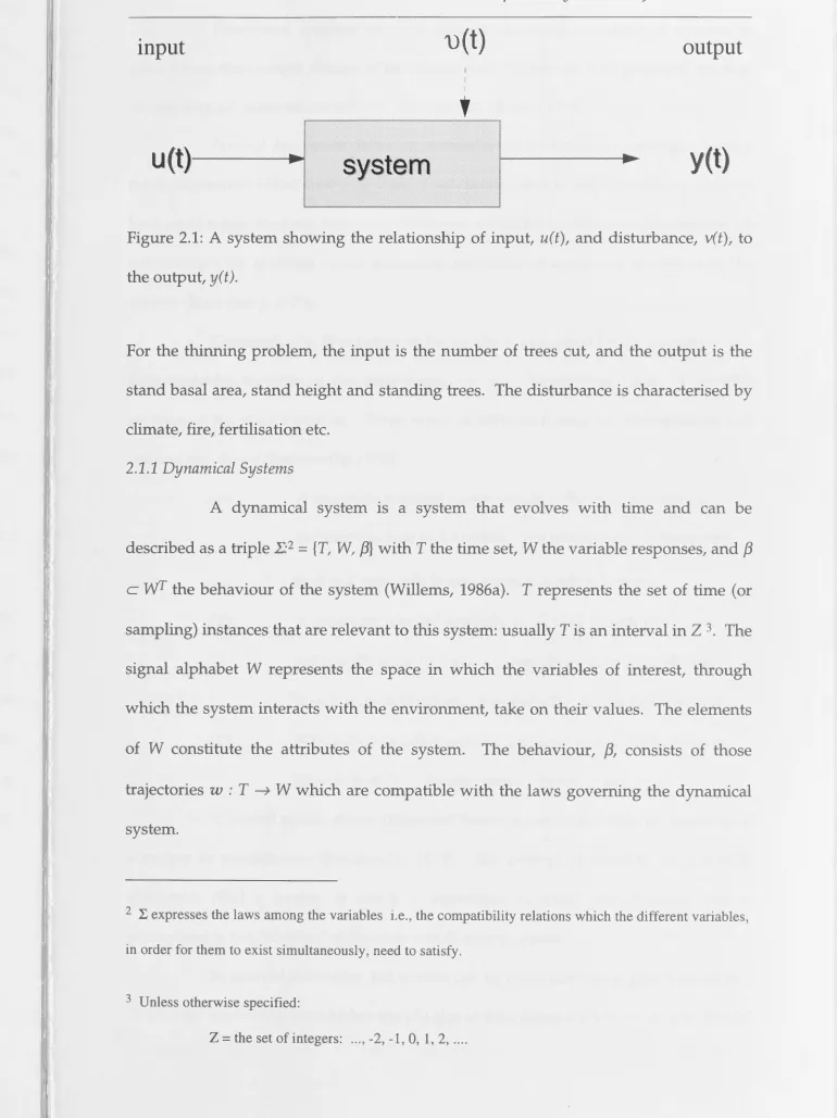
input and the external stimuli (disturbance or noise) that act on the system (see Figure
Chapter 2. System identification ll
input
u(t)
output
'
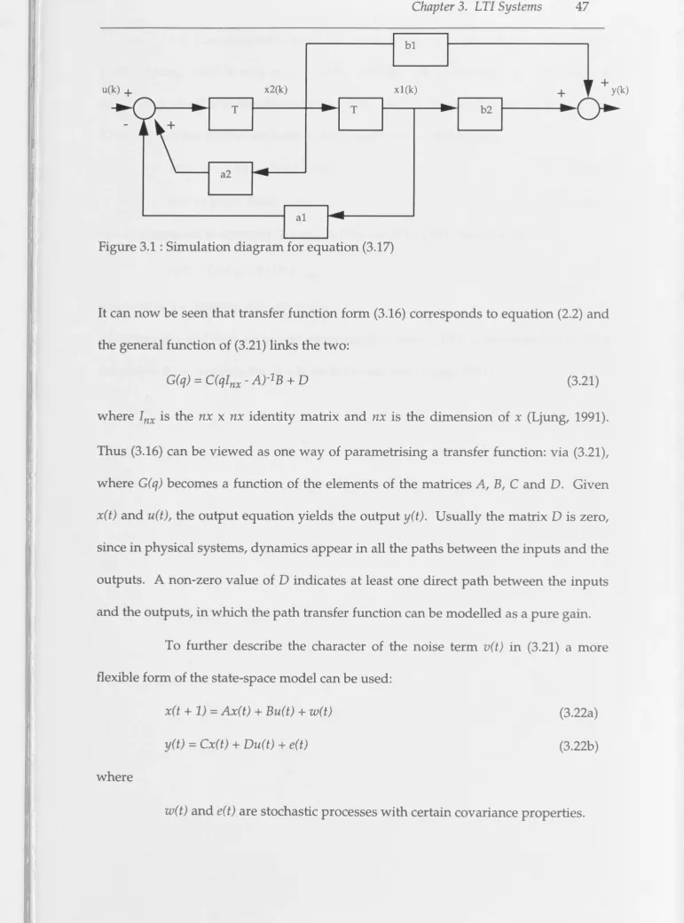
[image:22.786.0.770.38.1067.2]u(t)--~::
system
-
y(t)
Figure 2.1: A system showing the relationship of input, u(t), and disturbance, v(t), to
the output, y(t).
For the thinning problem, the input is the number of trees cut, and the output is the stand basal area, stand height and standing trees. The disturbance is characterised by
climate, fire, fertilisation etc.
2.1.1 Dynamical Systems
A dynamical system is a system that evolves with time and can be described as a triple .E:2
=
{T, W,/3}
with T the time set, W the variable responses, and/3
c WT the behaviour of the system (Willems, 1986a). T represents the set of time (or sampling) instances that are relevant to this system: usually Tis an interval in Z 3. The signal alphabet W represents the space in which the variables of interest, through which the system interacts with the environment, take on their values. The elements of W constitute the attributes of the system. The behaviour,
/3,
consists of those trajectories w : T ~ W which are compatible with the laws governing the dynamical system.2 L expresses the laws among the variables i.e., the compatibility relations
which the different variables,
in order for them to exist simultaneously, need to satisfy.
3 Unless otherwise specified:
Dynamical systems theory is concerned with the changes of systems in
time where the current change relies on the past. There are two principal ways of
description, i.e. internal and external descriptions (Rosen, 1971).
Internal description defines a system by all its internal couplings among a
set of n measures called state variables. Analytically, their change in time is expressed
by a set of n simultaneous first order difference equations (or differential equations for
continuous-time systems) called dynamical equations or equations of motion of the
system (Bertalanffy, 1973).
Geometrically, the change of the system is expressed by the trajectories the
state variables traverse in the state space, i.e. n
=
dimensional space of possiblelocation of the state variables. Three types of behaviour may be distinguished and
defined as follows (Bertalanffy, 1973):
(a) A trajectory is called asymptotically stable if all trajectories
sufficiently close to it at time,
t
=
to
(initial time) remain closeto it and approach it asymptotically when t --) 00 ;
(b) A trajectory is called neutrally stable if all trajectories
sufficiently close to it at
t
=
t
0, remain close to it for all latertime but do not necessarily approach it asymptotically; and
(c) A trajectory is called unstable if at least one of the trajectories
close to it at t
=
t0, do not remain close to it as t --) 00 •A central notion about dynamical theory is that of stability, i.e. response of
a system to perturbation (Bertalanffy, 1973). The concept of stability originates in
mechanics (that a motion is stable if insensitive to small perturbations) and is
generalised to the 'motions' of the state variables of a system.
In external description, the system can be considered as a 'grey box' or as a
Chapter 2. System identification 13
sets that have adjustable parameters with physical interpretation are called grey boxes.
In some cases standard models may be employed without reference to the physical
background. Such model sets whose parameters are basically viewed as vehicles for
adjusting the fit to the data and do not reflect physical considerations in the system,
are called black boxes (Ljung, 1987). A black box system description is typically
expressed in terms of input and output variables, via difference (or differential)
equations.
In principle it is usually possible to develop an internal description from
an external one and vice versa. In the case of linear systems formal techniques to
achieve this end are established (Willems, 1986a). When dealing with the general
nonlinear systems, such transformations are nontrivial. One moves from an internal
description to an external one by eliminating the state variables from the system
equation. By appropriately identifying a state variable defined via external variables
the external description can be transformed into an internal description.
In the context of system identification in particular where the physical
laws describing the system are too complex, external descriptions are easily obtained
and may be derived from data directly. It is essential to ensure that system
identification techniques lead to approximate system representations where the
quality of a model, depending on the objective of the modelling exercise, is expressed
by its predictive, simulation or control capabilities.
2.1.2 System Identification procedure
A dynamical model in discrete-time may be mathematically expressed as a
difference equation. In practice, circumstances usually do not allow an exact
mathematical representation of a system. However, if valid assumptions are made on
the system properties, a great deal of valuable information can be gained (Kuo, 1962).
To clarify the statement just made, it should be realised that all dynamical systems are
extremely difficult. Therefore, it is often necessary to assume that the system under
study behaves linearly over a range of operational conditions. The accuracy ( or
closeness to the truth) of the models can be improved by increasing the complexity of
the equations, but exactness (absolute truth) cannot be achieved. Therefore, it is
important to strive to develop a model that is adequate for the problem at hand
without making it overly complex. In some cases the assumption of linearity may
depart greatly from reality.
The procedure to determine a model of a dynamical system from observed
input/ output data involves three basic ingredients:
(a) the (input/ output) data;
(b) a set of candidate models ( the model structures); and
(c) a criterion to select a particular model in the set, based on the
information in the data (Ljung, 1991).
The input/ output data are sometimes recorded during a specifically
designed identification experiment, where the user makes a choice on what to
measure (signals) and when to measure (sampling instants) over some sampling
interval. The object with experimental design is thus to make these choices so that the
data becomes maximally informative. The key to success lies in:
(a) obtaining good quality data;
(b) a good knowledge (of the physics and/or ecology) of the
system; and
(c) having a good feel for the character of the model structure that
should be used (Ljung, 1987).
Without a reasonable data record not much can be done and there are
several reasons why such a record cannot be obtained in certain applications. A quite
obvious reason is that the time scale of the process is so slow that any informative data
Chapter 2. System identification 15
this problem. Another reason is that the input may not be open to manipulations.
Even if the manipulation of the input and measurement for long periods is possible, it
may be difficult to obtain a good data set. The prime reason for this is the presence of
unmeasurable disturbances that do not fit well into the standard picture of stochastic
processes.
The set of candidate models is obtained by specifying from which
collection of models4 to look for a suitable one. This is the most important and most
difficult part of the system identification procedure because it calls for:
(a) a priori knowledge and mathematical intuition; and
(b) an insight into modelling, e.g. constructing a model with some
unknown physical parameters from basic laws of nature and
other well established relationships or applying standard
linear models without reference to the physical background of
the system.
The 'best' model in the set is determined by applying diagnostic checks with the object
of uncovering possible lack of fit and diagnosing the cause. This can normally be
achieved by checking the mean squared error on how predictive the model is against
fresh data that were not used to construct the model. A bad choice of a model
structure cannot offer a good model, regardless of the amount and quality of the data.
Some processes will admit standard, ready-made (black box) model descriptions and
some, tailor-made model sets. In the latter, some physical insight is required before a
model can be estimated. This problem is clearly application dependent.
The identification process involves searching for a model structure by
computing the best model in the set and evaluating its properties to see if they are
satisfactory. The process can be listed as follows:
(a) Design an experiment and collect input/ output data;
(b) Examine the data; remove trends5 and outliers;
(c) Select and define a model from a set of candidate system
descriptions within which a model is to be found;
(d) Compute the best model according to (a) and a given criterion
of fit;
(e) Examine the obtained model's properties by checking against
fresh data; and
(f) If the model is good enough, then stop; OR go back to (c); OR
go back to (d); OR work further on (a) and (b).
It cannot, however, be sufficiently stressed that the key to successful
modelling lies in thinking, intuition and insight; these cannot be made obsolete by
automated model estimation.
2.2 The Linear Model Description
This section describes the way of mathematically defining the behavioural
patterns of linear dynamical systems. It is only when the dynamic characteristics of a
system are understood that intelligent direction, manipulation and control of the
system is possible. Concentration is on causal time-invariant linear systems, that were
found to be of great importance in deriving models that could accurately describe
suitable forest growth trends (Chikumbo et al., 1992; Chikumbo et al., 1993; Chikumbo
and Mareels, 1993; 1995a; 1995b). The growth models developed in this thesis were
nonlinear, but were characterised by linear time-invariant model structures as the
5 Care should be taken in removal of trends or detrending as this is applicable only to special types of
data. An example included in Endnote 2A illustrates the error that can result from inappropriate use of
Chapter 2. System identification 17
main building blocks. The following procedure was successfully adopted in
constructing the growth models:
(a) recognise linear-like responses and model these using
time-invariant linear model;
(b) recognise the critical system parameters that influence the
responses from the model in (a) and estimate them as linear
regression or polynomial functions;
(c) fit the functions from (b) to the model in (a) to give a
robust model.
Consider a system with a scalar input signal, u(t); t= 1, 2, ... , N, and a scalar
output signal y(t). The system is said to be time-invariant if its response to a certain
input signal does not depend on absolute time (Ljung, 1987). It is said to be linear if its
output response to a linear combination of inputs is the same linear combination of the
output responses of the individual inputs.
Introduction of the transfer function and impulse response concepts assists
in understanding linear system description. The modes of description are related and
each offers advantages and disadvantages in different fields of application and
circumstances (Box and Jenkins, 1971).
Let y(t) be represented as a function of the past values of u(t) and noise v(t), thus:
y(t)
=
g0u(t) + g1u(t-1) + g2u(t-2) + ... + v(t)(2.1)
or in shorthand,
y(t)
=
G(q)u(t) + v(t)(2.2)
where G(q)
=
g0 + g1q-1 + g2q-2 + ... , and q-1 is the backward shift operator defined as
qu(t)
=
u(t-1) and v(t) is a random variable with mean zero, a fixed covariancethe impulse response weights and a graph of these weights is called an impulse response
function.
Suppose that u is held indefinitely at some value, and the total change in y
is observed; the change in y(t) represents the sum of the impulse response weights, gk,
k
=
0, 1, 2, .... Therefore, this imposes a restriction that~
G(l)
=
Lgk < 00 (2.3)k=O
The value G(l) is the steady state gain of the system and it represents the total change in
y(t) for a unit change in u(t) held indefinitely at some new value (Vandaele, 1975). The
unit change in u(t), is a step change and the response that results from a step change is
an impulse response for a continuous-time system or pulse response for a
discrete-time system. A system that satisfies (2.2) is said to be stable, if the infinite series g0 +
g
1q
-
1 +g
2q
-
2 + ... converges for Iq
I ~ 1. Stability implies that a finite change in the inputresults in a finite change in the output. Thus for a stable system the sum of the
impulse response weights converges and is equal to the steady state gain of the system
(Box and Jenkins, 1971).
Under general conditions G(q) can be either approximated or exactly
represented by a ratio of two finite polynomials in
q:
G( )
=
B(q)q A(q) (2.4)
(2.5)
(2.6)
Without loss of generality the coefficient a0 can be normalised as unity. Equation (2.2)
thus becomes:
y(t)
=
B(q) u(t) + v(t)Chapter 2. System identification 19
It is possible that a delay or dead time, in the system's response can be present. To take
into account this generality -c, the dead time, is introduced to indicate the number of
periods it takes before u(t) starts influencing y(t). The transfer function model (2.7)
may then be written as:
y(t)
=
B(q) u(t - -r) + v(t)A(q)
In equation (2.2), v(t) can often be described as filtered white noise6 :
v(t)
=
H(q)e(t)where e(t) is white noise and
00
H(q)
=
Lh(k)q-kk=O
(2.8)
(2.9)
(2.10)
Noise can be a result of drift of the sensors that measure the signals or the influence of
signals that have the character of inputs but are not controlled by the observer. The
numbers {h(k)} are transfer functions from e toy. Equations (2.2) and (2.9) combined,
will thus become:
y(t) = G(q)u(t) + H(q)e(t) (2.11)
2.3 Modelling for Simulation, Prediction and Control
Objectives of a modelling exercise should be made clear at the outset so
that the effort spent in developing a model of a system is related to the application it is
intended for. After objectives have been set, selection of the most appropriate type of
model to achieve these objectives is carried out and decisions are made on the type of
modelling approach to use. This section considers three approaches in modelling
namely simulation, prediction and control. Throughout this section the system
description is assumed to take the form of equation (2.11).
Responses to various input scenarios {u*(t), t
=
1, 2, ... , N} are simulated.The undisturbed output will be as follows:
y*(t)
=
G(q)u*(t), t=
1, 2, ... , N (2.12)To evaluate the disturbance influence, a random generator is used to produce a
sequence of numbers e*(t), t
=
1, 2, ... , N, that can be used as a realisation of a whitenoise stochastic process with variance l. Hence
v*(t)
=
H(q)e*(t) (2.13)By presenting y*(t) and v*(t), an idea of the system response to u*(t) can be formed
(Ljung, 1987).
This way of experimenting on the model (2.11) rather than on the observed
physical process to evaluate its behaviour under different conditions (various input
scenarios) has become widely used in forestry, e.g. simulating silvicultural regimes
that have not been applied before.
2.3.2 Prediction
Consider the descriptions (2.9) and (2.11) and assume that y(s) and u(s) are
known for s ~t - 2. Since v(s)
=
y(s) - G(q)u(s), it also means that v(s) are known fors ~t - 2.
From (2.2) the conditional expectation of y(t) can be given as:
I\
y(t It - 1)
=
G(q)u(t) + v(tl t - 1)=
G(q)u(t) + [1 -H-l(q)Jv(t)=
G(q)u(t) + [1 - H-l(q)J[y(t) - G(q)u(t)Jy(t It -1)
=
H -1 (q)G(q)u(t) + [1 - H -1 (q)]y(t) (2.14)or
6 White noise defines disturbance or movement generated by independently distributed random variables
Chapter 2. System identification 21
H(q)y(t It -1)
=
G(q)u(t) + [H(q) - l]y(t) (2.15)Note that these expressions are shorthand notation for expansions. For
00
G(z)
example, let l(k) be defined by H(z) - L, l(k)z -k , and assume this is well defined for
k=O
I z I ;;? 1; H(z) has no zeros and G(z) no poles in I z I ;;? 1. Thus (2.14) means that
A = =
y(t It - 1)
=
L, l(k)u(t - k) + L,-h(k) y(t - k) (2.16)k=l k=l
The equations (2.14-16) make an assumption that the whole data record from time
minus infinity to t -1 is available. In practice, however, it is usually the case that only
data over the interval [O, t - 1] are known. The simplest thing to do would be to
replace the unknown data (Ljung, 1987). This is achieved by an approximation of the
actual conditional expectation of y(t), given data over [O, t - l]. The exact prediction
involves time-varying filter coefficients and can be computed using the
Wiener-Kalman-Bucy filter (Athans and Falb, 1966; Barnett and Cameron, 1985; Ljung, 1987).
A
From (2.11) and (2.14) the prediction error y(t) - y(t It - 1) is given by
ly(t) - ;(t It -1) = -H-l(q)G(q)u(t) + H-l(q)y(t) = e(t)I (2.17)
The variable e(t) thus represents that part of the output y(t) that cannot be predicted
from past data.
2.3.3 Control-Optimal
When considering physical systems, there are always some definite
objectives in the forefront and the aim is to accomplish some given task as 'cheaply' as
possible. In other words, the desire is to obtain the 'best' output which makes some
cost measure (or performance) large or small. The translation of these objectives into
the abstract language of dynamical systems gives rise to what is known as the control
(a) a dynamical system to be 'controlled';
(b) a desired output or objective of the system;
(c) a set of allowable (or admissible) 'controls' (i.e. inputs); and
(e) a performance or cost functional that measures the
effectiveness of a given 'control action'.
The essential elements arise out of the physical control-system design
problem. The mathematical model which represents the physical system, has been
examined in the preceding sections of this chapter, with the related concepts of input,
output and state. Thus in a more general way the problem addresses the control of a
dynamical system.
In translating a design problem into a control problem, one is faced with
the task of describing desirable physical behaviour in mathematical terms. The
objective of the system is often translated into a requirement on the output. The
control signals in physical systems cannot take on completely arbitrary values but are
subject to certain constraints. For example one cannot harvest more than the number
of trees in a forest and it is also not practical to harvest just one tree at a given time.
Constraints are thus imposed upon the inputs to the system. These constraints lead to
a set of admissible inputs (Athans and Falb, 1966; Boltyanskii, 1962).
Frequently the desired objective can be attained by many admissible
inputs, and so the designer seeks a measure of performance or cost of control that will
allow for choosing the 'best' input. Most of the time the cost functional chosen will
depend on the input and the pertinent variables (Elgerd, 1967). When a cost
functional has been decided upon, the designer formulates the control problem as
follows: Determine the admissible inputs which generate the desired output and
which, in so doing, optimise the chosen performance measure. At this point
optimal-control theory enters into the picture to aid the designer in finding a solution to the
Chapter 2. System identification 23
The word optimum may refer to either a maximum or a rrurumum
depending on the situation at hand (Elgerd, 1967; Maine and Iliff, 1985). The most
obvious method of optimisation is an outright search process for all possible solutions
in the total set of possible ones until the best one is found. Optimal control design
methods utilise, almost exclusively, state variables rather than transfer function
system descriptions, and therefore the index of performance as a rule will be
expressed as a scalar function, I, of the state and control-force vectors:
I= (2.18)
where
x= (x1(t), x2(t), ... , xn-1(t)), represents the state; and
u
=
(u1(t), u2(t), ... , ur(t)), the control parameters.The only constraints imposed upon the solution are those that relate to the physical
restrictions on the magnitudes of the components of x and u, i.e. x(t + 1)
=
Ftf x(t), u(t)J,t= 0, 1, ... , N - 2. Thus no a priori assumptions are made as to the system configuration
or linearity of control strategy. Translating this formulation to a forestry problem of
developing an optimal thinning strategy for a plantation stand, x would be the state
vector with state variables such as basal area, height, etc; u, the thinning strategy; Ft,
the economic value of the retained crop at time t; and I, the harvesting cost (index of
performance).
By observing the magnitude of the constraints, a u solution is sought
which optimises the chosen I criterion. The system difference equation. x(t + 1)
=
Ftf x(t), u(t)J, and the prescribed initial and final states, x(O) and x(tJ>, must be observed.
There are also constraints that are imposed on the optimisation problem (see chapter
I
[,
Ii
[,
'
'
I
I
: ,.,
To recapitulate, a control problem is the translation of a control system
design problem into mathematical terms; the solution of a control problem serves as a
guide in developing the actual working control system (Athans and Falb, 1966). More
on this topic is found in appendix II.
2.4 Arguments for dynamical models
Single equation regression models for tree growth are used to interpolate7
and extrapolate8 movements in a response variable by relating it to a set of
independent variables in an associative framework. Interpolation and extrapolation in
dynamical models are based on the dynamics of the response variable (output) that
are influenced by the input and the external stimuli.
Consider a time function g(t) which might represent an increment of some
tree stand attribute such as average stand diameter. It may or may not be possible to
explain (based on the observational parameters, i.e. external stimuli acting on the tree
stand system that the observer has no control over, such as drainage, exposure, soil
fertility and weather conditions) why g(t) behaved the way it did. Much of the
increment over time may have been due to factors that simply may not be explained or
accounted for, i.e. data are not available for those explanatory variables that are
believed to affect g(t). Even if data for all the variables that influence g(t) are available,
ill conditioning (or multicollinearity in the predictor variables) may be a problem.
7 Interpolation means prediction for new cases with independent variables not too different from values
of the independent variables in the construction sample (Weisberg, 1985). Interpolation is used
synonymously with simulation in this thesis. For a model, interpolation generally occurs when the
predictor is in the range observed in the construction sample.
8 Extrapolation is when the independent variable is estimated out of range of the observed data that was
Chapter 2. System identification 25
This is when one or more explanatory variables can be exactly expressed as a linear
combination (with various numerical coefficients) of other variables.
Assuming ill conditioning is not a problem, the estimation of a regression
model for g(t) might result in standard errors that are so large as to make most of the
estimated coefficients unreliable (Pindyck and Rubinfeld, 1981). Even if a statistically
significant regression equation for g(t) could be estimated, the result may not be useful
for interpolation and extrapolation. This could be attributed to any or all of the
following reasons:
(a) Statistical inferences derived from least squares regression
normally require that the residuals satisfy the Central Limit
Theorem. If this is violated robust regression methods such as
ridge regression or Maximum Likelihood Estimation can be
employed. The only problem is that up to now, no paradigm
has been developed that will specifically advocate a particular
treatment for problems that require robust regression (Draper
and Smith, 1981).
(b) The plot of the residuals against the predicted variable, g(t), or
explanatory variables may not be conforming to the 'horizontal
band' but indicating nonlinearity not accounted for by the
model or an increasing variance over time (Draper and Smith,
1981). Such a model would certainly not be reliable for
predictive purposes; maybe for simulation, but only if the
standard errors of the estimated coefficients of the model are
small, i.e. when the fit of the model to the data is good.
Possible remedies include transformation of the variables or
(c) The explanatory variables that are not lagged (or delayed)
may themselves have to be estimated, and this may be more
difficult than estimating g(t) itself (Pindyck and Rubinfeld,
1981). The standard error of the estimate of g(t) with expected
values of the known explanatory variables may be small (if the
regression equation fits well). However, when the expected
values of the explanatory variables are unknown, their
estimation errors may be so large as to make the estimation for
g(t) unacceptable.
Let's look, for instance, at a conventional growth model that is used by
many foresters for predicting stand basal area of a plantation species on known
productivity sites (identified by stand predominant heights at some specific age of a
forest). The Sullivan and Clutter (1972) stand basal area model (2.19) based on the
Schumacher (1939) model has a structure with two unspecified parameters (C1 and C2)
that can be fitted by means of data:
where
BAF Exp [ ~: lnBA1 + C1 (
1 -
~J
+C
2 (1
-
~:
J
S]
BA1
=
initial stand basal area (m2 ha-1)BA2
=
final stand basal area (m2 ha-1)A 1
=
initial stand age (years)A2
=
final stand age (years)S
=
site index (i.e. dominant height (m) at age 20)ln
=
natural logarithmsC1 and C2
=
coefficients.Chapter 2. System identification 27
Suppose there is lack of fit between data and model (2.19), and it has been
verified that this lack of fit is not due to randomness or data variance but that the
modelling structure is not capable of adequately explaining the observed trend. The
modelling exercise then becomes one of altering the model structure.
The model (2.19) can be expressed as follows:
(2.20)
where
From equation (2.20) it is easy to see that model (2.19) has no shape parameter other
than A2k that determines the maximum value of stand basal area. This makes model
(2.19) inflexible in representing a class of models. There is also no obvious systematic
means of increasing the parametric complexity of model (2.19) so that it can capture a
more complex trend. An attempt to increase its parametric complexity can be difficult
to formulate and time consuming; the potential of statistical and mathematical
complexity is high. It may not be inconceivable to select a completely different
modelling structure with all the drawbacks this entails.
It is no wonder model (2.19) could not be reliably used to model thinned
stands, even after incorporating a thinning correction factor (Brack, 1985; Chikumbo,
1991; McMullan, 1978). However, Knoebel et al., (1986) overcame this thinning
problem by using three models with model structure (2.19) parameterised for:
(a) before thinning;
(b) after first thinning; and
( c) after second and subsequent thinnings.
Thinning alters the shape of the basal area trend and a nonlinear function is desirable
that is sensitive to changes in stand density, and is capable of mapping the
corresponding changes in the basal area trend. In this dissertation such a model
A dynamical model, in contrast, comes from a class of 'flexible' model sets
(see chapter three) that can explain a variety of system behaviours without looking
into their internal structures. These model sets have increasing levels of parametric
complexity with corresponding capabilities of capturing increasing complex
behaviour in trends. As a result if one modelling structure is unsuitable, the next level
can be easily and promptly tried.
The simplest dynamical model (first order) such as the mean stand
diameter model (2.21) developed by Chikumbo et al., (1992) has two parameters, a and
b, that control shape and scale of the mean stand diameter trend respectively:
Dm(t)=aDm(t-1) + b(l-a) (2.21)
where
Dm
=
mean stand diameter (cm)There is thus a level of flexibility in model (2.21) that is not achievable in model (2.19).
Another popular growth function used often by foresters is the von
Bertalanffy's generalised Chapman-Richards' model that represent a family of curves
and is as follows:
y(t)
=
b(l-e-at)C (2.22)where y(t) is the growth response, b, the asymptotic value of biological carrying
capacity, a, the shape parameter, and c, the point of inflection in the growth curve.
Model (2.22) is essentially a dynamical model in continuous-time and in discrete-time
it becomes:
[y(t)]l/c
=
e-aT [y(t -1)]1/c+
b(l- e-aT) (2.23)where T
=
one time period.Chapter 2. System identification 29
aHe-aT ·
I
b(l - a) H b(l - e -aT); and
However, data acquisition in forestry (or any other discipline) is in discrete-time and it
follows that discrete-time model development is adequate. Ratkowsky (1983)
demonstrated that the least squares estimates of the parameters a and c in model (2.22)
undergo considerable variation making it hard to estimate them. This is because
model (2.22) requires detailed sampled data to estimate its parameters. Such data are
expensive to obtain.
This parameter instability led Ratkowsky (1983) to recommend
'reparameterisation' where one of the offending (sensitive) parameters is expressed as
a function of the other parameters of the same model, without the expression
containing the explanatory variables or the error term. Maximum likelihood
estimation can be used for specifying the loss function or the objective function to
maximise (Press et. al., 1992). Nonlinear least squares routines (Press et. al., 1992) such
as the Levenberg-Marquardt method (also called Marquardt method) can be
employed for the gradient search, because of their increased robustness and iterative
efficiency.
Growth and yield models in forestry are mostly used for projection; forest
planners want to know, with reasonable accuracy, the response of a tree crop to
improved stock, cuttings, different densities etc., (Dargavel,
J.
per. comm., 1992). Dataused for modelling are always collected from a particular site or sites and crops are
well looked after which is atypical in the plantations or natural forests. Structural
models developed from these data may not behave as expected when used for