ELECTROMAGNETICS
VT Publishing
Blacksburg, Virginia
ELECTROMAGNETICS
STEVEN W. ELLINGSON
This textbook is licensed with a Creative Commons Attribution Share-Alike 4.0 license https://creativecommons.org/licenses/by-sa/4.0. You are free to copy, share, adapt, remix, transform and build upon the material for any purpose, even commercially as long as you follow the terms of the license https://creativecommons.org/licenses/by-sa/4.0/legalcode.
You must:
Attribute — You must give appropriate credit, provide a link to the license, and indicate if changes were made. You may do so in any reasonable manner, but not in any way that suggests the licensor endorses you or your use.
Suggested citation: Ellingson, Steven W. (2018) Electromagnetics, Vol. 1. Blacksburg, VA: VT Publishing. https://doi.org/10.21061/electromagnetics-vol-1 Licensed with CC BY-SA 4.0 https://creativecommons.org/licenses/by-sa/4.0
ShareAlike — If you remix, transform, or build upon the material, you must distribute your contributions under the same license as the original.
You may not:
Add any additional restrictions — You may not apply legal terms or technological measures that legally restrict others from doing anything the license permits.
This work is published by VT Publishing, a division of University Libraries at Virginia Tech, 560 Drillfield Drive, Blacksburg, VA 24061, USA [email protected].
The print version of this book is printed in the United States of America. Publication Cataloging Information
Ellingson, Steven W., author
Electromagnetics (Volume 1) / Steven W. Ellingson Pages cm
ISBN 978-0-9979201-8-5 (print) ISBN 978-0-9979201-9-2 (ebook)
DOI: https://doi.org/10.21061/electromagnetics-vol-1 1. Electromagnetism. 2. Electromagnetic theory. I. Title
QC760.E445 2018 621.3
Cover Design: Robert Browder
Cover Image: © Michelle Yost. Total Internal Reflection https://flic.kr/p/dWAhx5 is licensed with a Creative Commons Attribution-ShareAlike 2.0 license https://creativecommons.org/licenses/by-sa/2.0/ (cropped by Robert Browder)
What is an Open Textbook?
Open textbooks are complete textbooks that have been funded, published, and licensed to be freely used, adapted, and distributed. As a particular type of Open Educational Resource (OER), this open textbook is intended to provide authoritative, accurate, and comprehensive subject content at no cost, to anyone including those who utilize technology to read and those who cannot afford traditional textbooks. This book is licensed with a Creative Commons Share-Alike 4.0 license (see p. iv.), which allows it to be adapted, remixed, and shared under the same license with attribution. Instructors and other readers may be interested in localizing, rearranging, or adapting content, or in transforming the content into other formats with the goal of better addressing student learning needs, and/or making use of various teaching methods.
Open textbooks in a variety of disciplines are available via the Open Textbook Library: https://open.umn.edu/opentextbooks.
Feedback Requested
The editor and author of this book seek content-related suggestions from faculty, students, and others using the book. Methods for providing feedback are presented in the User Feedback Guide at:
http://bit.ly/userfeedbackguide
• Submit suggestions (anonymous) http://bit.ly/electromagnetics-suggestion
• Annotate using Hypothes.is http://web.hypothes.is (instructions are in the feedback guide) • Send suggestions via email: [email protected]
Additional Resources
These following resources for Electromagnetics Vol 1 are available at: http://hdl.handle.net/10919/84164 • Downloadable PDF of the text
• Source files (LaTeX tarball) • Errata for Volume 1
• Problem sets & solution manual
• Information for book’s community portal and listserv
If you are a professor reviewing, adopting, or adapting this textbook please help us understand a little more about your use by filling out this form: http://bit-ly/vtpublishing-updates
Contents
Preface xii
1 Preliminary Concepts 1
1.1 What is Electromagnetics? . . . 1
1.2 Electromagnetic Spectrum . . . 3
1.3 Fundamentals of Waves . . . 5
1.4 Guided and Unguided Waves . . . 9
1.5 Phasors . . . 9
1.6 Units . . . 13
1.7 Notation . . . 15
2 Electric and Magnetic Fields 17 2.1 What is a Field? . . . 17
2.2 Electric Field Intensity . . . 17
2.3 Permittivity . . . 20
2.4 Electric Flux Density . . . 21
2.5 Magnetic Flux Density . . . 22
2.6 Permeability . . . 25
2.7 Magnetic Field Intensity . . . 26
2.8 Electromagnetic Properties of Materials . . . 27
CONTENTS vii
3 Transmission Lines 30
3.1 Introduction to Transmission Lines . . . 30
3.2 Types of Transmission Lines . . . 31
3.3 Transmission Lines as Two-Port Devices . . . 33
3.4 Lumped-Element Model . . . 34
3.5 Telegrapher’s Equations . . . 35
3.6 Wave Equation for a TEM Transmission Line . . . 37
3.7 Characteristic Impedance . . . 38
3.8 Wave Propagation on a TEM Transmission Line . . . 39
3.9 Lossless and Low-Loss Transmission Lines . . . 41
3.10 Coaxial Line . . . 42
3.11 Microstrip Line . . . 44
3.12 Voltage Reflection Coefficient . . . 47
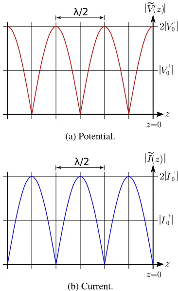
3.13 Standing Waves . . . 49
3.14 Standing Wave Ratio . . . 51
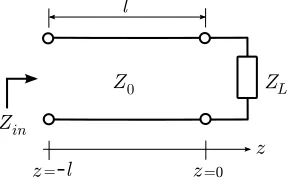
3.15 Input Impedance of a Terminated Lossless Transmission Line . . . 52
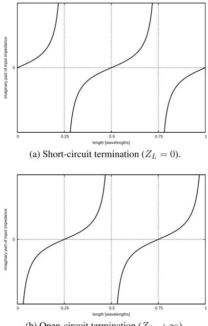
3.16 Input Impedance for Open- and Short-Circuit Terminations . . . 54
3.17 Applications of Open- and Short-Circuited Transmission Line Stubs . . . 55
3.18 Measurement of Transmission Line Characteristics . . . 56
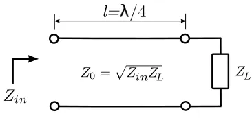
3.19 Quarter-Wavelength Transmission Line . . . 57
3.20 Power Flow on Transmission Lines . . . 60
3.21 Impedance Matching: General Considerations . . . 62
3.22 Single-Reactance Matching . . . 63
3.23 Single-Stub Matching . . . 66
4 Vector Analysis 70 4.1 Vector Arithmetic . . . 70
4.3 Cylindrical Coordinates . . . 77
4.4 Spherical Coordinates . . . 81
4.5 Gradient . . . 84
4.6 Divergence . . . 85
4.7 Divergence Theorem . . . 87
4.8 Curl . . . 88
4.9 Stokes’ Theorem . . . 90
4.10 The Laplacian Operator . . . 91
5 Electrostatics 93 5.1 Coulomb’s Law . . . 93
5.2 Electric Field Due to Point Charges . . . 95
5.3 Charge Distributions . . . 95
5.4 Electric Field Due to a Continuous Distribution of Charge . . . 96
5.5 Gauss’ Law: Integral Form . . . 100
5.6 Electric Field Due to an Infinite Line Charge using Gauss’ Law . . . 101
5.7 Gauss’ Law: Differential Form . . . 103
5.8 Force, Energy, and Potential Difference . . . 105
5.9 Independence of Path . . . 107
5.10 Kirchoff’s Voltage Law for Electrostatics: Integral Form . . . 108
5.11 Kirchoff’s Voltage Law for Electrostatics: Differential Form . . . 109
5.12 Electric Potential Field Due to Point Charges . . . 110
5.13 Electric Potential Field due to a Continuous Distribution of Charge . . . 112
5.14 Electric Field as the Gradient of Potential . . . 113
5.15 Poisson’s and Laplace’s Equations . . . 115
5.16 Potential Field Within a Parallel Plate Capacitor . . . 116
5.17 Boundary Conditions on the Electric Field Intensity (E) . . . 118
CONTENTS ix
5.19 Charge and Electric Field for a Perfectly Conducting Region . . . 122
5.20 Dielectric Media . . . 123
5.21 Dielectric Breakdown . . . 124
5.22 Capacitance . . . 124
5.23 The Thin Parallel Plate Capacitor . . . 126
5.24 Capacitance of a Coaxial Structure . . . 128
5.25 Electrostatic Energy . . . 130
6 Steady Current and Conductivity 134 6.1 Convection and Conduction Currents . . . 134
6.2 Current Distributions . . . 135
6.3 Conductivity . . . 136
6.4 Resistance . . . 138
6.5 Conductance . . . 141
6.6 Power Dissipation in Conducting Media . . . 143
7 Magnetostatics 146 7.1 Comparison of Electrostatics and Magnetostatics . . . 146
7.2 Gauss’ Law for Magnetic Fields: Integral Form . . . 147
7.3 Gauss’ Law for Magnetism: Differential Form . . . 148
7.4 Ampere’s Circuital Law (Magnetostatics): Integral Form . . . 149
7.5 Magnetic Field of an Infinitely-Long Straight Current-Bearing Wire . . . 150
7.6 Magnetic Field Inside a Straight Coil . . . 152
7.7 Magnetic Field of a Toroidal Coil . . . 155
7.8 Magnetic Field of an Infinite Current Sheet . . . 157
7.9 Ampere’s Law (Magnetostatics): Differential Form . . . 159
7.10 Boundary Conditions on the Magnetic Flux Density (B) . . . 160
7.12 Inductance . . . 163
7.13 Inductance of a Straight Coil . . . 165
7.14 Inductance of a Coaxial Structure . . . 167
7.15 Magnetic Energy . . . 169
7.16 Magnetic Materials . . . 170
8 Time-Varying Fields 174 8.1 Comparison of Static and Time-Varying Electromagnetics . . . 174
8.2 Electromagnetic Induction . . . 175
8.3 Faraday’s Law . . . 178
8.4 Induction in a Motionless Loop . . . 180
8.5 Transformers: Principle of Operation . . . 183
8.6 Transformers as Two-Port Devices . . . 185
8.7 The Electric Generator . . . 187
8.8 The Maxwell-Faraday Equation . . . 189
8.9 Displacement Current and Ampere’s Law . . . 190
9 Plane Waves in Lossless Media 194 9.1 Maxwell’s Equations in Differential Phasor Form . . . 194
9.2 Wave Equations for Source-Free and Lossless Regions . . . 196
9.3 Types of Waves . . . 198
9.4 Uniform Plane Waves: Derivation . . . 199
9.5 Uniform Plane Waves: Characteristics . . . 203
9.6 Wave Polarization . . . 206
9.7 Wave Power in a Lossless Medium . . . 209
A Constitutive Parameters of Some Common Materials 213 A.1 Permittivity of Some Common Materials . . . 213
CONTENTS xi
A.3 Conductivity of Some Common Materials . . . 215
B Mathematical Formulas 217
B.1 Trigonometry . . . 217
B.2 Vector Operators . . . 217
B.3 Vector Identities . . . 219
C Physical Constants 220
Preface
About This Book
[m0146]
Goals for this book.This book is intended to serve as a primary textbook for a one-semester introductory course in undergraduate engineering
electromagnetics, including the following topics: electric and magnetic fields; electromagnetic properties of materials; electromagnetic waves; and devices that operate according to associated electromagnetic principles including resistors, capacitors, inductors, transformers, generators, and transmission lines.
This book employs the “transmission lines first” approach, in which transmission lines are introduced using a lumped-element equivalent circuit model for a differential length of transmission line, leading to one-dimensional wave equations for voltage and current.1 This is sufficient to address transmission
line concepts, including characteristic impedance, input impedance of terminated transmission lines, and impedance matching techniques. Attention then turns to electrostatics, magnetostatics, time-varying fields, and waves, in that order.
What’s new.This version of the book is thesecond public release of this book. The first release, known as “Volume 1 (Beta),” was released in January 2018. Improvements from the beta version include the following:
• Correction of errors identified in the beta version errata and many minor improvements.
• Addition of an index.
1Are you an instructor who is not a fan of the “transmission
lines first” approach? Then see “What are those little numbers
in square brackets?” later in this section.
• Accessibility features: Figures now include “alt text” suitable for screen reading software.
• Addition of a separate manual of examples and solutions (see the web site).
• Addition of source files for the book (see the web site).
Target audience.This book is intended for electrical engineering students in the third year of a bachelor of science degree program. It is assumed that readers are familiar with the fundamentals of electric circuits and linear systems, which are normally taught in the second year of the degree program. It is also assumed that readers have received training in basic
engineering mathematics, including complex numbers, trigonometry, vectors, partial differential equations, and multivariate calculus. Review of the relevant principles is provided at various points in the text. In a few cases (e.g., phasors, vectors) this review consists of a separate stand-alone section.
Notation, examples, and highlights.Section 1.7 summarizes the mathematical notation used in this book. Examples are set apart from the main text as follows:
Example 0.1. This is an example.
“Highlight boxes” are used to identify key ideas as follows:
This is a key idea.
What are those little numbers in square brackets? This book is a product of the
Open Electromagnetics Project. This project provides a large number of sections (“modules”) which are
xiii
assembled (“remixed”) to create new and different versions of the book. The text “[m0146]” that you see at the beginning of this section uniquely identifies the module within the larger set of modules provided by the project. This identification is provided because different remixes of this book may exist, each consisting of a different subset and arrangement of these modules. Prospective authors can use this identification as an aid in creating their own remixes.
Why do some sections of this book seem to repeat material presented in previous sections?In some remixes of this book, authors might choose to eliminate or reorder modules. For this reason, the modules are written to “stand alone” as much as possible. As a result, there may be some redundancy between sections that would not be present in a traditional (non-remixable) textbook. While this may seem awkward to some at first, there are clear
benefits: In particular, it never hurts to review relevant past material before tackling a new concept. And, since the electronic version of this book is being offered at no cost, there is not much gained by eliminating this useful redundancy.
Why cite Wikipedia pages as additional reading? Many modules cite Wikipedia entries as sources of additional information. Wikipedia represents both the best and worst that the Internet has to offer. Most authors of traditional textbooks would agree that citing Wikipedia pages as primary sources is a bad idea, since quality is variable and content is subject to change over time. On the other hand, many Wikipedia pages are excellent, and serve as useful sources of relevant information that is not strictly within the scope of the curriculum. Furthermore, students benefit from seeing the same material presented differently, in a broader context, and with additional references cited by Wikipedia pages. We trust instructors and students to realize the potential pitfalls of this type of resource and to be alert for problems.
Acknowledgments.Here’s a list of talented and helpful people who contributed to this book:
The staff of VT Publishing, University Libraries, Virginia Tech:
Editor: Anita Walz
Advisors: Peter Potter, Corinne Guimont Cover: Robert Browder, Anita Walz
Other VT contributors:
Assessment: Tiffany Shoop, Anita Walz Accessibility: Christa Miller
Virginia Tech students:
Alt text writer: Stephanie Edwards Figure designer: Michaela Goldammer Figure designer: Kruthika Kikkeri Figure designer: Youmin Qin
Copyediting:
Melissa Ashman, Kwantlen Polytechnic University
External reviewers:
Samir El-Ghazaly, University of Arkansas Stephen Gedney, University of Colorado Denver Randy Haupt, Colorado School of Mines Karl Warnick, Brigham Young University
About the Open Electromagnetics
Project
[m0148]
TheOpen Electromagnetics Projectwas established at Virginia Tech in 2017 with the goal of creating no-cost openly-licensed textbooks for courses in undergraduate engineering electromagnetics. While a number of very fine traditional textbooks are available on this topic, we feel that it has become unreasonable to insist that students pay hundreds of dollars per book when effective alternatives can be provided using modern media at little or no cost to the student. This project is equally motivated by the desire for the freedom to adopt, modify, and improve educational resources. This work is distributed under a Creative Commons BY SA license which allows – and we hope encourages – others to adopt, modify, improve, and expand the scope of our work.
About the Author
[m0153]
Steven W. Ellingson ([email protected]) is an Associate Professor at Virginia Tech in Blacksburg, Virginia in the United States. He received PhD and MS degrees in Electrical Engineering from the Ohio State University and a BS in Electrical & Computer Engineering from Clarkson University. He was employed by the US Army, Booz-Allen & Hamilton, Raytheon, and the Ohio State University
Chapter 1
Preliminary Concepts
1.1
What is Electromagnetics?
[m0037]
The topic of this book is applied engineering
electromagnetics. This topic is often described as “the theory of electromagnetic fields and waves,” which is both true and misleading. The truth is that electric fields, magnetic fields, their sources, waves, and the behavior these waves are all topics covered by this book. The misleading part is that ourprincipalaim shall be to close the gap between basic electrical circuit theory and the more general theory that is required to address certain topics that are of broad and common interest in the field of electrical engineering. (For a preview of topics where these techniques are required, see the list at the end of this section.)
In basic electrical circuit theory, the behavior of devices and systems is abstracted in such a way that the underlying electromagnetic principles do not need to be considered. Every student of electrical
engineering encounters this, and is grateful since this greatly simplifies analysis and design. For example, a resistor is commonly defined as a device which exhibits a particular voltageV =IRin response to a currentI, and the resistor is thereforecompletely described by the valueR. This is an example of a “lumped element” abstraction of an electrical device. Much can be accomplished knowing nothing else about resistors; no particular knowledge of the physical concepts of electrical potential, conduction current, or resistance is required. However, this simplification makes it impossible to answer some frequently-encountered questions. Here are just a few:
• What determinesR? How does one go about designing a resistor to have a particular resistance?
• Practical resistors are rated for power-handling capability; e.g., discrete resistors are frequently identified as “1/8-W,” “1/4-W,” and so on. How does one determine this, and how can this be adjusted in the design?
• Practical resistors exhibit significant reactance as well as resistance. Why? How is this
determined? What can be done to mitigate this?
• Most things which are not resistors also exhibit significant resistance and reactance – for
example, electrical pins and interconnects. Why? How is this determined? What can be done to mitigate this?
The answers to the these questions must involve properties of materialsandthe geometry in which those materials are arranged. These are precisely the things that disappear in lumped element device models, so it is not surprising that such models leave us in the dark on these issues. It should also be apparent that what is true for the resistor is also going to be true for other devices of practical interest, including capacitors (and devices unintentionally exhibiting capacitance), inductors (and devices unintentionally exhibiting inductance), transformers (and devices unintentionally exhibiting mutual impedance), and so on. From this perspective, electromagnetics may be viewed as a generalization of electrical circuit theory that addresses these considerations. Conversely basic electric circuit theory may be viewed a special case of
electromagnetic theory that applies when these considerations are not important. Many instances of this “electromagnetics as generalization” vs. “lumped-element theory as special case” dichotomy appear in the study of electromagnetics.
There is more to the topic, however. There are many devices and applications in which electromagnetic fields and waves areprimaryengineering
considerations that must be dealt with directly. Examples include electrical generators and motors; antennas; printed circuit board stackup and layout; persistent storage of data (e.g., hard drives); fiber optics; and systems for radio, radar, remote sensing, and medical imaging. Considerations such as signal integrity and electromagnetic compatibility (EMC) similarly require explicit consideration of
electromagnetic principles.
Although electromagnetic considerations pertain to all frequencies, these considerations become increasingly difficult to avoid with increasing frequency. This is because the wavelength of an electromagnetic field decreases with increasing frequency.1 When wavelength is large compared to the size of the region of interest (e.g., a circuit), then analysis and design is not much different from zero-frequency (“DC”) analysis and design.
For example, the free space wavelength at 3 MHz is about 100 m, so a planar circuit having dimensions 10 cm×10 cm is just 0.1% of a wavelength across at this frequency. Although an electromagnetic wave may be present, it has about the same value over the region of space occupied by the circuit. In contrast, the free space wavelength at 3 GHz is about 10 cm, so the same circuit is one full wavelength across at this frequency. In this case, different parts of this circuit observe the same signal with very different magnitude and phase.
Some of the behaviors associated with non-negligible dimensions are undesirable, especially if not taken into account in the design process. However, these behaviors can also be exploited to do some amazing and useful things – for example, to launch an electromagnetic wave (i.e., an antenna) or to create
1Most readers have encountered the concepts of frequency and
wavelength previously, but can refer to Section 1.3, if needed, for a quick primer.
filters and impedance matching devices consisting only of metallic shapes, free of discrete capacitors or inductors.
Electromagnetic considerations become not only unavoidable but central to analysis and design above a few hundred MHz, and especially in the
millimeter-wave, infrared (IR), optical, and ultraviolet (UV) bands.2 The discipline of electrical engineering encompasses applications in these frequency ranges even though – ironically – such applications may not operate according to principles that can be considered “electrical”! Nevertheless, electromagnetic theory applies.
Another common way to answer the question “What is electromagnetics?” is to identify the topics that are commonly addressed within this discipline. Here’s a list of topics – some of which have already been mentioned – in which explicit consideration of electromagnetic principles is either important or essential:3
• Antennas
• Coaxial cable
• Design and characterization of common discrete passive components including resistors,
capacitors, inductors, and diodes
• Distributed (e.g., microstrip) filters
• Electromagnetic compatibility (EMC)
• Fiber optics
• Generators
• Magnetic resonance imaging (MRI)
• Magnetic storage (of data)
• Microstrip transmission lines
• Modeling of non-ideal behaviors of discrete components
• Motors
2See Section 1.2 for a quick primer on the electromagnetic
spec-trum and this terminology.
3Presented in alphabetical order so as to avoid the appearance of
1.2. ELECTROMAGNETIC SPECTRUM 3
• Non-contact sensors
• Photonics
• Printed circuit board stackup and layout
• Radar
• Radio wave propagation
• Radio frequency electronics
• Signal integrity
• Transformers
• Waveguides
In summary:
Applied engineering electromagnetics is the study of those aspects of electrical engineering in situations in which theelectromagnetic proper-ties of materialsandthe geometry in which those materials are arranged is important. This re-quires an understanding of electromagnetic fields and waves, which are ofprimaryinterest in some applications.
Finally, here are two broadly-defined learning objectives that should now be apparent: (1) Learn the techniques of engineering analysis and design that apply when electromagnetic principles are important, and (2) Better understand the physics underlying the operation of electrical devices and systems, so that when issues associated with these physical principles emerge one is prepared to recognize and grapple with them.
1.2
Electromagnetic Spectrum
[m0075]
Electromagnetic fields exist at frequencies from DC (0 Hz) to at least1020Hz – that’s at least 20 orders of magnitude!
At DC, electromagnetics consists of two distinct disciplines:electrostatics, concerned with electric fields; andmagnetostatics, concerned with magnetic fields.
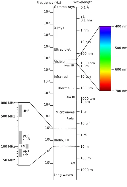
At higher frequencies, electric and magnetic fields interact to form propagating waves. Waves having frequencies within certain ranges are given names based on how they manifest as physical phenomena. These names are (in order of increasing frequency): radio,infrared(IR),optical(also known as “light”), ultraviolet(UV),X-rays, andgamma rays(γ-rays). See Table 1.1 and Figure 1.1 for frequency ranges and associated wavelengths.
The termelectromagnetic spectrum refers to the various forms of electromagnetic phenomena that exist over the continuum of frequencies.
The speed (properly known as “phase velocity”) at which electromagnetic fields propagate in free space is given the symbolc, and has the value
∼
= 3.00×10⁸m/s. This value is often referred to as the “speed of light.” While it is certainly the speed of light in free space, it is also speed ofany
electromagnetic wave in free space. Given frequency
f, wavelength is given by the expression
λ= c
f in free space
Table 1.1 shows the free space wavelengths associated with each of the regions of the electromagnetic spectrum.
Regime Frequency Range Wavelength Range
γ-Ray >3×10¹⁹Hz <0.01nm
X-Ray 3×10¹⁶Hz –3×10¹⁹Hz 10–0.01 nm
Ultraviolet (UV) 2.5×10¹⁵–3×10¹⁶Hz 120–10 nm
Optical 4.3×10¹⁴–2.5×10¹⁵Hz 700–120 nm
Infrared (IR) 300 GHz –4.3×10¹⁴Hz 1 mm – 700 nm
Radio 3 kHz – 300 GHz 100 km – 1 mm
Table 1.1: The electromagnetic spectrum. Note that the indicated ranges are arbitrary but consistent with common usage.
effects become important at frequencies as low as the optical, IR, or radio bands. (A prime example is the photoelectric effect; see “Additional References” below.) Thus, caution is required when applying the classical version of electromagnetic theory presented here, especially at these higher frequencies.
Theory presented in this book is applicable to DC, radio, IR, and optical waves, and to a lesser extent to UV waves, X-rays, andγ-rays. Cer-tain phenomena in these frequency ranges – in particular quantum mechanical effects – are not addressed in this book.
The radio portion of the electromagnetic spectrum alone spans 12 orders of magnitude in frequency (and wavelength), and so, not surprisingly, exhibits a broad range of phenomena. This is shown in Figure 1.1. For this reason, the radio spectrum is further subdivided into bands as shown in Table 1.2. Also shown in Table 1.2 are commonly-used band identification acronyms and some typical applications.
Similarly, the optical band is partitioned into the familiar “rainbow” of red through violet, as shown in Figure 1.1 and Table 1.3. Other portions of the spectrum are sometimes similarly subdivided in certain applications.
Additional Reading:
• “Electromagnetic spectrum” on Wikipedia.
• “Photoelectric effect” on Wikipedia.
400 nm
500 nm
600 nm
700 nm
1000 m 100 m 10 m 1 m 10 cm 1 cm 1 mm 1000 µm 100 µm 10 µm 1 µm 1000 nm 100 nm 10 nm 0.1 Å
0.1 nm 1Å
1 nm Wavelength
1017
1016
1015
1014
1013
1012
1011
1010
109
108
106 Frequency (Hz)
1018 1019
UHF
VHF 7-13
FM VHF 2-6 1000 MHz
500 MHz
100 MHz
50 MHz
Gamma-rays
X-rays
Ultraviolet
Visible
Near IR
Infra-red
Thermal IR
Far IR
Microwaves
Radar
Radio, TV
AM
Long-waves 107
c
[image:19.576.281.495.258.572.2]V. Blacus CC BY-SA 3.0
1.3. FUNDAMENTALS OF WAVES 5
Band Frequencies Wavelengths Typical Applications
EHF 30-300 GHz 10–1 mm 60 GHz WLAN, Point-to-point data links
SHF 3–30 GHz 10–1 cm Terrestrial & Satellite data links, Radar
UHF 300–3000 MHz 1–0.1 m TV broadcasting, Cellular, WLAN
VHF 30–300 MHz 10–1 m FM & TV broadcasting, LMR
HF 3–30 MHz 100–10 m Global terrestrial comm., CB Radio
MF 300–3000 kHz 1000–100 m AM broadcasting
LF 30–300 kHz 10–1 km Navigation, RFID
VLF 3–30 kHz 100–10 km Navigation
Table 1.2: The radio portion of the electromagnetic spectrum, according to a common scheme for naming ranges of radio frequencies. WLAN: Wireless local area network, LMR: Land mobile radio, RFID: Radio frequency identification.
Band Frequencies Wavelengths
Violet 668–789 THz 450–380 nm
Blue 606–668 THz 495–450 nm
Green 526–606 THz 570–495 nm
Yellow 508–526 THz 590–570 nm
Orange 484–508 THz 620–590 nm
Red 400–484 THz 750–620 nm
Table 1.3: The optical portion of the electromagnetic spectrum.
1.3
Fundamentals of Waves
[m0074]
In this section, we formally introduce the concept of a wave and explain some basic characteristics.
To begin, let us consider not electromagnetic waves, but rather sound waves. To be clear, sound waves and electromagnetic waves are completely distinct phenomena. Sound waves are variations in pressure, whereas electromagnetic waves are variations in electric and magnetic fields. However, the mathematics that govern sound waves and electromagnetic waves are very similar, so the analogy provides useful insight. Furthermore, sound waves are intuitive for most people because they are readily observed. So, here we go:
Imagine standing in an open field and that it is completely quiet. In this case, the air pressure everywhere is about 101 kPa (101,000 N/m2) at sea
level, and we refer to this as thequiescent air pressure. Sound can be described as thedifferential air pressurep(x, y, z, t), which we define as the absolute air pressure at the spatial coordinates
(x, y, z)minus the quiescent air pressure. So, when there is no sound,p(x, y, z, t) = 0. The functionpas an example of ascalar field.4
Let’s also say you are standing atx=y=z= 0and you have brought along a friend who is standing at
x=d; i.e., a distancedfrom you along thexaxis. Also, for simplicity, let us consider only what is happening along thexaxis; i.e.,p(x, t).
Att= 0, you clap your hands once. This forces the air between your hands to press outward, creating a region of increased pressure (i.e.,p >0) that travels outward. As the region of increased pressure moves outward, it leaves behind a region of low pressure wherep <0. Air molecules immediately move toward this region of lower pressure, and so the air pressure quickly returns to the quiescent value,p= 0. The traveling disturbance inp(x, t)is the sound of the clap. The disturbance continues to travel outward until it reaches your friend, who then hears the clap.
At each point in time, you can make a plot ofp(x, t)
versusxfor the current value oft. This is shown in Figure 1.2. At timest <0, we have simply
p(x, t) = 0. A short time aftert= 0, the peak pressure is located at slightly to the right ofx= 0. The pressure is not a simple impulse because interactions between air molecules constrain the
4Although it’s not important in this section, you can read about
p(x,t)
x
p(x,t)
x
c
Y. Qin CC BY 4.0
Figure 1.2: The differential pressurep(x, t)(top) a short time after the clap and (bottom) a slightly longer time after the clap.
pressure to be continuous over space. So instead, we see a rounded pulse representing the rapid build-up and similarly rapid decline in air pressure. A short time laterp(x, t)looks very similar, except the pulse is now further away.
Now: What precisely isp(x, t)? Completely skipping over the derivation, the answer is thatp(x, t)is the solution to theacoustic wave equation (see “Additional References” at the end of this section):
∂2p
∂x2− 1
c2
s ∂2p
∂t2 = 0 (1.1)
wherecsis the speed of sound, which is about 340 m/s at sea level. Just to emphasize the quality of the analogy between sound waves and
electromagnetic waves, know that the acoustic wave equation is mathematically identical to equations that that govern electromagnetic waves.
Although “transient” phenomena – analogous to a clap – are of interest in electromagnetics, an even more common case of interest is the wave resulting from a sinusoidally-varying source. We can
demonstrate this kind of wave in the context of sound as well. Here we go:
In the previous scenario, you pick up a trumpet and
blow a perfect A note. The A note is 440 Hz, meaning that the air pressure emerging from your trumpet is varying sinusoidally at a frequency of 440 Hz. Let’s say you can continue to blow this note long enough for the entire field to be filled with the sound of your trumpet. Now what does the pressure-versus-distance curve look like? Two simple observations will settle that question:
• p(x, t)at anyconstant positionxis a sinusoid as a function ofx. This is because the acoustic wave equation is linear and time invariant, so a sinusoidal excitation (i.e., your trumpet) results in a sinusoidal response at the same frequency (i.e., the sound heard by your friend).
• p(x, t)at anyconstant timetis also a sinusoid as a function ofx. This is because the sound is propagating away from the trumpet and toward your friend, and anyone in between will also hear the A note, but with a phase shift determined by the difference in distances.
This is enough information to know that the solution must have the form:
p(x, t) =Amcos (ωt−βx+ψ) (1.2)
whereω= 2πf,f = 440Hz, andAm,β, andψ remain to be determined.
You can readily verify that Equation 1.2 satisfies the acoustic wave equation when
β= ω
cs
(1.3)
In this problem, we findβ∼= 8.13rad/m. This means that at any given time, the difference in phase measured between any two points separated by a distance of 1 m is 8.13 rad. The parameterβgoes by at least three names:phase propagation constant, wavenumber, andspatial frequency. The term “spatial frequency” is particularly apt, sinceβplays precisely the same role for distance (x) asωplays for time (t) – This is apparent from Equation 1.2. However, “wavenumber” is probably the more commonly-used term.
1.3. FUNDAMENTALS OF WAVES 7
Note thatAmandψare not determined by the wave equation, but instead are properties of the source. Specifically,Amis determined by how hard we blow, andψis determined by the time at which we began to blow and the location of the trumpet. For simplicity, let us assume that we begin to blow at timet≪0; i.e., in the distant past so that the sound pressure field has achieved steady state byt= 0. Also, let us set
ψ= 0and setAm= 1in whatever units we choose to expressp(x, t). We then have:
p(x, t) = cos (ωt−βx) (1.4)
Now we have everything we need to make plots of
p(x)at various times.
Figure 1.3(a) showsp(x, t= 0). As expected,
p(x, t= 0)is periodic inx. The associated period is referred to as thewavelengthλ. Sinceλis the distance required for the phase of the wave to increase by2πrad, and because phase is increasing at a rate of
βrad/m, we find:
λ= 2π
β (1.5)
In the present example, we findλ∼= 77.3cm.
Wavelengthλ = 2π/β is the distance required for the phase of a sinusoidal wave to increase by one complete cycle (i.e.,2πrad) at any given time.
Now let us consider the situation att= +1/4f, which ist= 568µs andωt=π/2. We see in Figure 1.3(b) that the waveform has shifted a distance
λ/4to the right. It is in this sense that we say the wave is propagating in the+xdirection.
Furthermore, we can now compute aphase velocity
vp: We see that a point of constant phase has shifted a distanceλ/4in time1/4f, so
vp=λf (1.6)
In the present example, we findvp∼= 340m/s; i.e., we have found that the phase velocity is equal to the speed of soundcs. It is in this sense that we say that the phase velocity is the speed at which the wave propagates.5
5It is worth noting here is that “velocity” is technically a vector;
i.e., speed in a given direction. Nevertheless, this quantity is actually just a speed, and this particular abuse of terminology is generally accepted.
p(x,t)
x λ
p(x,t)
x
p(x,t)
x
c
Y. Qin CC BY 4.0
Figure 1.3: The differential pressurep(x, t) for (a)
Phase velocityvp = λf is the speed at which a point of constant phase in a sinusoidal waveform travels.
Recall that in Equation 1.2 we declared thatβxis subtracted from the argument of the sinusoidal function. To understand why, let’s change the sign of
βxand see if it still satisfies the wave equation – one finds that it does. Next, we repeat the previous experiment and see what happens. The result is shown in Figure 1.3(c). Note that points of constant phase have traveled an equal distance, but now in the−x
direction. In other words, this alternative choice of sign forβxwithin the argument of the cosine function represents a wave that is propagating in the opposite direction. This leads us to the following realization:
If the phase of the wave is decreasing withβx, then the wave is propagating in the+xdirection. If the phase of the wave is increasing with βx, then the wave is propagating in the−xdirection.
Since the prospect of sound traveling toward the trumpet is clearly nonsense in the present situation, we may neglect the latter possibility. However, what happens if there is a wall located in the distance, behind your friend? Then, we expect an echo from the wall, which would be a second wave propagating in the reverse direction and for which the argument of the cosine function would contain the term “+βx.”
Finally, let us return to electromagnetics.
Electromagnetic waves satisfy precisely the same wave equation (i.e., Equation 1.1) as do sound waves, except that the phase velocity is much greater. Interestingly, though, the frequencies of
electromagnetic waves are also much greater than those of sound waves, so we can end up with wavelengths having similar orders of magnitude. In particular, an electromagnetic wave withλ= 77.3cm (the wavelength of the “A” note in the preceding example) lies in the radio portion of the
electromagnetic spectrum.
An important difference between sound and
electromagnetic waves is that electromagnetic waves are vectors; that is, they havedirectionas well as magnitude. Furthermore, we often need to consider multiple electromagnetic vector waves (in particular,
both theelectric fieldand themagnetic field) in order to completely understand the situation. Nevertheless the concepts of wavenumber, wavelength, phase velocity, and direction of propagation apply in precisely the same manner to electromagnetic waves as they do to sound waves.
Additional Reading:
• “Wave Equation” on Wikipedia.
1.4. GUIDED AND UNGUIDED WAVES 9
1.4
Guided and Unguided Waves
[m0040]
Broadly speaking, waves may be eitherguidedor unguided.
Unguided waves include those that are radiated by antennas, as well as those that are unintentionally radiated. Once initiated, these waves propagate in an uncontrolled manner until they are redirected by scattering or dissipated by losses associated with materials.
Examples of guided waves are those that exist within structures such as transmission lines, waveguides, and optical fibers. We refer to these as guided because they are constrained to follow the path defined by the structure.
Antennas and unintentional radiators emit un-guided waves. Transmission lines, waveguides, and optical fibers carryguided waves.
1.5
Phasors
[m0033]
In many areas of engineering, signals are
well-modeled as sinusoids. Also, devices that process these signals are often well-modeled as linear time-invariant (LTI) systems. The response of an LTI system to any linear combination of sinusoids is another linear combination of sinusoids having the same frequencies.6In other words, (1) sinusoidal
signals processed by LTI systems remain sinusoids and are not somehow transformed into square waves or some other waveform; and (2) we may calculate the response of the system for one sinusoid at a time, and then add the results to find the response of the system when multiple sinusoids are applied simultaneously. This property of LTI systems is known assuperposition.
The analysis of systems that process sinusoidal waveforms is greatly simplified when the sinusoids are represented asphasors. Here is the key idea:
Aphasoris a complex-valued number that repre-sents a real-valued sinusoidal waveform. Specif-ically, a phasor has the magnitude and phase of the sinusoid it represents.
Figures 1.4 and 1.5 show some examples of phasors and the associated sinusoids.
It is important to note that a phasor by itself is not the signal. A phasor is merely a simplified mathematical representation in which the actual, real-valued physical signal is represented as a complex-valued constant.
Here is a completely general form for a physical (hence, real-valued) quantity varying sinusoidally with angular frequencyω= 2πf:
A(t;ω) =Am(ω) cos (ωt+ψ(ω)) (1.7)
whereAm(ω)is magnitude at the specified frequency, ψ(ω)is phase at the specified frequency, andtis time. Also, we require∂Am/∂t= 0; that is, that the time
6A “linear combination” of functionsfi(t)wherei= 1,2,3, ...
Amej
magnitu de Im{C}
Re{C}
Am phase ( )
-jAm
Am-jBm
Bm
Figure 1.4: Examples of phasors, displayed here as points in the real-imaginary plane.
variation ofA(t)is completely represented by the cosine function alone. Now we can equivalently expressA(t;ω)as a phasorC(ω):
C(ω) =Am(ω)ejψ(ω) (1.8)
To convert this phasor back to the physical signal it represents, we (1) restore the time dependence by multiplying byejωt, and then (2) take the real part of the result. In mathematical notation:
A(t;ω) =ReC(ω)ejωt (1.9)
To see why this works, simply substitute the right hand side of Equation 1.8 into Equation 1.9. Then:
A(t) =Re
n
Am(ω)ejψ(ω)ejωt
o
=RenAm(ω)ej(ωt+ψ(ω))
o
=Re{Am(ω) [cos (ωt+ψ(ω))
+jsin (ωt+ψ(ω))]}
=Am(ω) cos (ωt+ψ(ω))
as expected.
It is common to write Equation 1.8 as follows, dropping the explicit indication of frequency
t
t
t
A
mA
me
jψA
m-
jB
mt
-
jA
mnote slightly larger amplitude
note now a sine function
1.5. PHASORS 11
dependence:
C=Amejψ (1.10)
This does not normally cause any confusion since the definition of a phasor requires that values ofCandψ
are those that apply at whatever frequency is
represented by the suppressed sinusoidal dependence
ejωt.
Table 1.4 shows mathematical representations of the same phasors demonstrated in Figure 1.4 (and their associated sinusoidal waveforms in Figure 1.5). It is a good exercise is to confirm each row in the table, transforming from left to right and vice-versa.
It is not necessary to use a phasor to represent a sinusoidal signal. We choose to do so because phasor representation leads to dramatic simplifications. For example:
• Calculation of the peak value from data representingA(t;ω)requires a time-domain search over one period of the sinusoid. However, if you knowC, the peak value ofA(t)is simply
|C|, and no search is required.
• Calculation ofψfrom data representingA(t;ω)
requires correlation (essentially, integration) over one period of the sinusoid. However, if you knowC, thenψis simply the phase ofC, and no integration is required.
Furthermore, mathematical operations applied to
A(t;ω)can be equivalently performed as operations onC, and the latter are typically much easier than the former. To demonstrate this, we first make two important claims and show that they are true.
Claim 1: LetC1andC2be two complex-valued constants (independent oft). Also,
ReC1ejωt =Re
C2ejωt for allt. Then,
C1=C2.
Proof:Evaluating att= 0we find
Re{C1}=Re{C2}. SinceC1andC2are constant with respect to time, this must be true for allt. At
t=π/(2ω)we find
ReC1ejωt =Re{C1·j}=−Im{C1}
and similarly
ReC2ejωt =Re{C2·j}=−Im{C2}
therefore Im{C1}=Im{C2}. Once again: SinceC1 andC2are constant with respect to time, this must be true for allt. Since the real and imaginary parts ofC1 andC2are equal,C1=C2.
What does this mean?We have just shown that if two phasors are equal, then the sinusoidal waveforms that they represent are also equal.
Claim 2: For any real-valued linear operatorT and complex-valued quantityC,
T(Re{C}) =Re{T(C)}.
Proof:LetC=cr+jciwherecrandciare real-valued quantities, and evaluate the right side of the equation:
Re{T(C)}=Re{T(cr+jci)}
=Re{T(cr) +jT(ci)}
=T(cr)
=T(Re{C})
What does this mean?The operators that we have in mind forT include addition, multiplication by a constant, differentiation, integration, and so on. Here’s an example with differentiation:
Re
∂
∂ωC
=Re
∂
∂ω(cr+jci)
= ∂
∂ωcr
∂
∂ωRe{C}= ∂
∂ωRe{(cr+jci)}= ∂ ∂ωcr
A(t) C
Amcos (ωt) Am
Amcos (ωt+ψ) Amejψ Amsin (ωt) =Amcos ωt−π2 −jAm Amcos (ωt) +Bmsin (ωt) =Amcos (ωt) +Bmcos ωt−π2 Am−jBm
Table 1.4: Some examples of physical (real-valued) sinusoidal signals and the corresponding phasors.Amand Bmare real-valued and constant with respect tot.
Summarizing:
Claims 1 and 2 together entitle us to perform op-erations on phasors as surrogates for the physi-cal, real-valued, sinusoidal waveforms they rep-resent. Once we are done, we can transform the resulting phasor back into the physical waveform it represents using Equation 1.9, if desired.
However, a final transformation back to the time domain is usuallynotdesired, since the phasor tells us everything we can know about the corresponding sinusoid.
A skeptical student might question the value of phasor analysis on the basis that signals of practical interest are sometimes not sinusoidally-varying, and therefore phasor analysis seems not to apply generally. It is certainly true that many signals of practical interest are not sinusoidal, and many are far from it. Nevertheless, phasor analysisisbroadly applicable. There are basically two reasons why this is so:
• Many signals, although not strictly sinusoidal, are “narrowband” and therefore well-modeled as sinusoidal. For example, a cellular
telecommunications signal might have a bandwidth on the order of 10 MHz and a center frequency of about 2 GHz. This means the difference in frequency between the band edges of this signal is just 0.5% of the center
frequency. The frequency response associated with signal propagation or with hardware can often be assumed to be constant over this range of frequencies. With some caveats, doing phasor analysis at the center frequency and assuming the results apply equally well over the bandwidth of interest is often a pretty good approximation.
• It turns out that phasor analysis is easily extensible to any physical signal, regardless of bandwidth. This is so because any physical signal can be decomposed into a linear combination of sinusoids – this is known as Fourier analysis. The way to find this linear combination of sinusoids is by computing the Fourier series, if the signal is periodic, or the Fourier Transform, otherwise. Phasor analysis applies to each frequency independently, and (invoking superposition) the results can be added together to obtain the result for the complete signal. The process of combining results after phasor analysis results is nothing more than integration over frequency; i.e.:
Z +∞
−∞
A(t;ω)dω
Using Equation 1.9, this can be rewritten:
Z +∞
−∞
ReC(ω)ejωt dω
We can go one step further using Claim 2:
Re
Z +∞
−∞
C(ω)ejωtdω
The quantity in the curly braces is simply the Fourier transform ofC(ω). Thus, we see that we can analyze a signal of arbitrarily-large
bandwidth simply by keepingωas an
1.6. UNITS 13
Summarizing:
Phasor analysis does not limit us to sinusoidal waveforms. Phasor analysis is not only applica-ble to sinusoids and signals that are sufficiently narrowband, but is also applicable to signals of arbitrary bandwidth via Fourier analysis.
Additional Reading:
• “Phasor” on Wikipedia.
• “Fourier analysis” on Wikipedia.
1.6
Units
[m0072]
The term “unit” refers to the measure used to express a physical quantity. For example, the mean radius of the Earth is about 6,371,000 meters; in this case the unit is the meter.
A number like “6,371,000” becomes a bit
cumbersome to write, so it is common to use a prefix to modify the unit. For example, the radius of the Earth is more commonly said to be 6371 kilometers, where one kilometer is understood to mean
1000 meters. It is common practice to use prefixes, such as “kilo-,” that yield values in the range0.001to
10,000. A list of standard prefixes appears in Table 1.5.
Writing out the names of units can also become tedious. For this reason, it is common to use standard abbreviations; e.g., “6731 km” as opposed to
“6371 kilometers,” where “k” is the standard abbreviation for the prefix “kilo” and “m” is the standard abbreviation for “meter.” A list of
commonly-used base units and their abbreviations are shown in Table 1.6.
To avoid ambiguity, it is important to always indicate the units of a quantity; e.g., writing “6371 km” as opposed to “6371.” Failure to do so is a common source of error and misunderstandings. An example is
Prefix Abbreviation Multiply by:
exa E 1018
peta P 1015
tera T 1012
giga G 109
mega M 106
kilo k 103
milli m 10−3
micro µ 10−6
nano n 10−9
pico p 10−12
femto f 10−15
atto a 10−18
Unit Abbreviation Quantifies:
ampere A electric current
coulomb C electric charge
farad F capacitance
henry H inductance
hertz Hz frequency
joule J energy
meter m distance
newton N force
ohm Ω resistance
second s time
tesla T magnetic flux density
volt V electric potential
watt W power
weber Wb magnetic flux
Table 1.6: Some units that are commonly used in elec-tromagnetics.
the expression:
l= 3t
wherelis length andtis time. It could be thatlis in meters andtis in seconds, in which case “3” really means “3 m/s”. However, if it is intended thatlis in kilometers andtis in hours, then “3” really means “3 km/h” and the equation is literally different. To patch this up, one might write “l= 3tm/s”; however, note that this does does not resolve the ambiguity we just identified – i.e., we still don’t know the units of the constant “3.” Alternatively, one might write “l= 3twherelis in meters andtis in seconds,” which is unambiguous but becomes quite awkward for more complicated expressions. A better solution is to write instead:
l= (3m/s)t
or even better:
l=at wherea= 3m/s
since this separates this issue of units from the perhaps more-important fact thatlis proportional tot
and the constant of proportionality (a) is known.
The meter is the fundamental unit of length in the International System of Units, known by its French acronym “SI” and sometimes informally referred to as the “metric system.”
In this work, we will use SI units exclusively.
Although SI is probably the most popular for engineering use overall, other systems remain in common use. For example, the English system, where the radius of the Earth might alternatively be said to be about 3959 miles, continues to be used in various applications and to a lesser or greater extent in various regions of the world. An alternative system in common use in physics and material science
applications is the CGS (“centimeter-gram-second”) system. The CGS system is similar to SI, but with some significant differences. For example, the base unit of energy is the CGS system is not the “joule” but rather the “erg,” and the values of some physical constants become unitless. Therefore – once again – it is very important to include units whenever values are stated.
SI defines seven fundamental units from which all other units can be derived. These fundamental units are distance in meters (m), time in seconds (s), current in amperes (A), mass in kilograms (kg), temperature in kelvin (K), particle count in moles (mol), and luminosity in candela (cd). SI units for electromagnetic quantities such as coulombs (C) for charge and volts (V) for electric potential are derived from these fundamental units.
A frequently-overlooked feature of units is their ability to assist in error-checking mathematical expressions. For example, the electric field intensity may be specified in volts per meter (V/m), so an expression for the electric field intensity that yields units of V/m is said to be “dimensionally correct” (but not necessarily correct), whereas an expression that cannot be reduced to units of V/mcannotbe correct.
Additional Reading:
• “International System of Units” on Wikipedia.
1.7. NOTATION 15
1.7
Notation
[m0005]
The list below describes notation used in this book.
• Vectors: Boldface is used to indicate a vector; e.g., the electric field intensity vector will typically appear asE. Quantities not in boldface are scalars. When writing by hand, it is common to write “E” or “−→E” in lieu of “E.”
• Unit vectors: A circumflex is used to indicate a unit vector; i.e., a vector having magnitude equal to one. For example, the unit vector pointing in the+xdirection will be indicated asx. Inˆ
discussion, the quantity “x” is typically spokenˆ
“xhat.”
• Time: The symboltis used to indicate time.
• Position: The symbols(x, y, z),(ρ, φ, z), and
(r, θ, φ)indicate positions using the Cartesian, cylindrical, and polar coordinate systems, respectively. It is sometimes convenient to express position in a manner which is
independent of a coordinate system; in this case, we typically use the symbolr. For example, r= ˆxx+ ˆyy+ ˆzzin the Cartesian coordinate system.
• Phasors:A tilde is used to indicate a phasor quantity; e.g., a voltage phasor might be indicated asVe, and the phasor representation of Ewill be indicated asE.e
• Curves, surfaces, and volumes:These
geometrical entities will usually be indicated in script; e.g., an open surface might be indicated asSand the curve bounding this surface might be indicated asC. Similarly, the volume enclosed by a closed surfaceSmay be indicated asV.
• Integrations over curves, surfaces, and volumes will usually be indicated using a single integral sign with the appropriate subscript. For example:
Z
C· · ·
dl is an integral over the curveC
Z
S· · ·
ds is an integral over the surfaceS
Z
V· · ·
dv is an integral over the volumeV.
• Integrations over closed curves and surfaceswill be indicated using a circle superimposed on the integral sign. For example:
I
C· · ·
dl is an integral over the closed curveC
I
S
···ds is an integral over the closed surfaceS
A “closed curve” is one which forms an unbroken loop; e.g., a circle. A “closed surface” is one which encloses a volume with no openings; e.g., a sphere.
• The symbol “∼=” means “approximately equal to.” This symbol is used when equality exists, but is not being expressed with exact numerical precision. For example, the ratio of the
circumference of a circle to its diameter isπ, whereπ∼= 3.14.
• The symbol “≈” also indicates “approximately equal to,” but in this case the two quantities are unequal even if expressed with exact numerical precision. For example,ex= 1 +x+x2/2 +...
as a infinite series, butex≈1 +xforx≪1. Using this approximatione0.1≈1.1, which is in good agreement with the actual value
e0.1∼= 1.1052.
• The symbol “∼” indicates “on the order of,” which is a relatively weak statement of equality indicating that the indicated quantity is within a factor of 10 or so the indicated value. For example,µ∼105for a class of iron alloys, with exact values being being larger or smaller by a factor of 5 or so.
• The symbol “,” means “is defined as” or “is equal as the result of a definition.”
• Complex numbers:j,√−1.
• See Appendix C for notation used to identify commonly-used physical constants.
Image Credits
Fig. 1.1 cV. Blacus, https://commons.wikimedia.org/wiki/File:Electromagnetic-Spectrum.svg, CC BY SA 3.0 (https://creativecommons.org/licenses/by-sa/3.0/).
Fig. 1.2: cY. Qin, https://commons.wikimedia.org/wiki/File:M0074 fClap.svg, CC BY 4.0 (https://creativecommons.org/licenses/by/4.0/).
Chapter 2
Electric and Magnetic Fields
2.1
What is a Field?
[m0001]
A field is the continuum of values of a quantity as a function of position and time.
The quantity that the field describes may be a scalar or a vector, and the scalar part may be either real- or complex-valued.
In electromagnetics, the electric field intensityEis a real-valued vector field that may vary as a function of position and time, and so might be indicated as “E(x, y, z, t),” “E(r, t),” or simply “E.” When expressed as a phasor, this quantity is complex-valued but exhibits no time dependence, so we might say instead “Ee(r)” or simply “Ee.”
An example of a scalar field in electromagnetics is the electric potential,V; i.e.,V(r, t).
Awaveis a time-varying field that continues to exist in the absence of the source that created it and is therefore able to transport energy.
2.2
Electric Field Intensity
[m0002]
Electric field intensityis a vector field we assign the symbolEand has units of electrical potential per distance; in SI units, volts per meter (V/m). Before offering a formal definition, it is useful to consider the broader concept of theelectric field.
Imagine that the universe is empty except for a single particle of positive charge. Next, imagine that a second positively-charged particle appears; the situation is now as shown in Figure 2.1. Since like charges repel, the second particle will be repelled by the first particle and vice versa. Specifically, the first particle isexerting forceon the second particle. If the second particle is free to move, it will do so; this is an expression of kinetic energy. If the second particle is somehow held in place, we say the second particle possesses an equal amount of potential energy. This potential energy is no less “real,” since we can convert it to kinetic energy simply by releasing the particle, thereby allowing it to move.
Now let us revisit the original one particle scenario.
F
c
M. Goldammer CC BY SA 4.0
Figure 2.1: A positively-charged particle experiences a repulsive forceFin the presence of another particle which is also positively-charged.
F
c
M. Goldammer CC BY SA 4.0
Figure 2.2: A map of the force that would be expe-rienced by a second particle having a positive charge. Here, the magnitude and direction of the force is indi-cated by the size and direction of the arrow.
In that scenario, we could make a map in which every position in space is assigned a vector that describes the force that a particle having a specified chargeq
would experience if it were to appear there. The result looks something like Figure 2.2. This map of force vectors is essentially a description of the electric field associated with the first particle.
There are many ways in which the electric field may be quantified. Electric field intensityEis simply one of these ways. We defineE(r)to be the forceF(r)
experienced by a test particle having chargeq, divided byq; i.e.,
E(r), lim
q→0 F(r)
q (2.1)
Note that it is required for the charge to become vanishingly small (as indicated by taking the limit) in order for this definition to work. This is because the source of the electric field is charge, so the test particle contributes to the total electric field. To accurately measure the field of interest, the test charge must be small enough not to significantly perturb the field. This makes Equation 2.1 awkward from an engineering perspective, and we’ll address that later in this section.
According the definition of Equation 2.1, the units of Eare those of force divided by charge. The SI units for force and charge are the newton (N) and coulomb
(C) respectively, soEhas units of N/C. However, we typically expressEin units of V/m, not N/C. What’s going on? The short answer is that 1 V/m=1 N/C:
N
C =
N·m C·m =
J C·m=
V m
where we have used the fact that 1 N·m=1 joule (J) of energy and 1 J/C=1 V.
Electric field intensity (E, N/C or V/m) is a vec-tor field that quantifies the force experienced by a charged particle due to the influence of charge not associated with that particle.
The analysis of units doesn’t do much to answer the question of why we should prefer to expressEin V/m as opposed to N/C. Let us now tackle that question.
Figure 2.3 shows a simple thought experiment that demonstrates the concept of electric field intensity in terms of an electric circuit. This circuit consists of a parallel-plate capacitor in series with a 9 V battery.1
The effect of the battery, connected as shown, is to force an accumulation of positive charge on the upper plate, and an accumulation of negative charge on the lower plate. If we consider the path from the position labeled “A,” along the wire and through the battery to the position labeled “B,” the change in electric potential is+9V. It must also be true that the change in electric potential as we travel from B to A through the capacitor is−9V, since the sum of voltages over any closed loop in a circuit is zero. Said differently, the change in electric potential between the plates of the capacitor, starting from node A and ending at node B, is+9V. Now, note that the spacing between the plates in the capacitor is 1 mm. Thus, the rate of change of the potential between the plates is 9 V divided by 1 mm, which is 9000 V/m. This is literally the electric field intensity between the plates. That is, if one places a particle with an infinitesimally-small charge between the plates (point “C”), and then measures the ratio of force to charge, one finds it is 9000 N/C pointing toward A. We come to the following remarkable conclusion:
1It is not necessary to know anything about capacitors to get to
2.2. ELECTRIC FIELD INTENSITY 19
A B
+
-9V
1mm
c
Y. Qin CC BY 3.0
Figure 2.3: A simple circuit used to describe the con-cept of electric field intensity. In this example,E at point C is 9000 V/m directed from B toward A.
Epoints in the direction in which electric poten-tial is most rapidly decreasing, and the magnitude ofEis the rate of change in electric potential with distance in this direction.
The reader may have noticed that we have defined the electric field in terms of what itdoes. We have have not directly addressed the question of what the electric fieldis. This is the best we can do using classical physics, and fortunately, this is completely adequate for the most engineering applications. However, a deeper understanding is possible using quantum mechanics, where we find that the electric field and the magnetic field are in fact manifestations of the same fundamental force, aptly named the electromagnetic force. (In fact, the electromagnetic force is found to be one of just four fundamental forces, the others beinggravity, thestrong nuclear force, and theweak nuclear force.) Quantum mechanics also facilitates greater insight into the nature of electric charge and of thephoton, which is the fundamental constituent of electromagnetic waves. For more information on this topic, an excellent starting point is the video “Quantum Invariance & The Origin of The Standard Model” referenced at the end of this section.
Additional Reading:
• “Electric field” on Wikipedia.
• PBS Space Time video “Quantum Invariance &
2.3
Permittivity
[m0008]
Permittivity describes the effect of material in determining the electric field in response to electric charge. For example, one can observe from laboratory experiments that a particle having chargeqgives rise to the electric field
E= ˆRq 1
4πR2 1
ǫ (2.2)
whereRis distance from the charge,Rˆ is a unit vector pointing away from the charge, andǫis a constant that depends on the material. Note thatE increases withq, which makes sense since electric charge is the source ofE. Also note thatEis inversely proportional to4πR2, indicating thatE decreases in proportion to the area of a sphere surrounding the charge – a principle commonly known as theinverse square law. The remaining factor1/ǫis the constant of proportionality, which captures the effect of material. Given units of V/m for Eand C forQ, we find thatǫmust have units of farads per meter (F/m). (To see this, note that 1 F=
1 C/V.)
Permittivity (ǫ, F/m) describes the effect of ma-terial in determining the electric field intensity in response to charge.
In free space (that is, a perfect vacuum), we find that
ǫ=ǫ0where:
ǫ0∼= 8.854×10⁻¹²F/m (2.3)
The permittivity of air is only slightly greater, and usually can be assumed to be equal to that of free space. In most other materials, the permittivity is significantly greater; that is, the same charge results in a weaker electric field intensity.
It is common practice to describe the permittivity of materials relative to the permittivity of free space. Thisrelative permittivity is given by:
ǫr, ǫ ǫ0
(2.4)
Values ofǫrfor a few representative materials is given in Appendix A.1. Note thatǫrranges from 1
(corresponding to a perfect vacuum) to about 60 or so in common engineering applications. Also note that relative permittivity is sometimes referred to as dielectric constant. This term is a bit misleading, however, since permittivity is a meaningful concept for many materials that are not dielectrics.
Additional Reading:
• “Permittivity” on Wikipedia.
• Appendix A.1 (“Permittivity of Some Common Materials”).
2.4. ELECTRIC FLUX DENSITY 21
2.4
Electric Flux Density
[m0011]
Electric flux density, assigned the symbolD, is an alternative to electric field intensity (E) as a way to quantify an electric field. This alternative description offers some actionable insight, as we shall point out at the end of this section.
First, what is electric flux density? Recall that a particle having chargeqgives rise to the electric field intensity
E= ˆRq 1
4πR2 1
ǫ (2.5)
whereRis distance from the charge andRˆ points away from the charge. Note thatEis inversely proportional to4πR2, indicating thatEdecreases in proportion to the area of a sphere surrounding the charge. Now integrate both sides of Equation 2.5 over a sphereSof radiusR:
I
S
E(r)·ds= I
S
ˆ
Rq 1
4πR2 1
ǫ
·ds (2.6)
Factoring out constants that do not vary with the variables of integration, the right-hand side becomes:
q 1
4πR2 1
ǫ
I
S
ˆ
R·ds
Note thatds= ˆRdsin this case, and also that
ˆ
R·Rˆ = 1. Thus, the right-hand side simplifies to:
q 1
4πR2 1
ǫ
I
S
ds
The remaining integral is simply the area ofS, which is4πR2. Thus, we find:
I
S
E(r)·ds= q
ǫ (2.7)
The integral of a vector field over a specified surface is known asflux(see “Additional Reading” at the end of this section). Thus, we have found that the flux of Ethrough the sphereSis equal to a constant, namely
q/ǫ. Furthermore, this constant is the same regardless of the radiusRof the sphere. Said differently, the flux ofEis constant with distance, and does not vary asE itself does. Let us capitalize on this observation by
making the following small modification to
Equation 2.7: I
S
[ǫE]·ds=q (2.8)
In other words, the flux of the quantityǫEis equal to the enclosed charge, regardless of the radius of the sphere over which we are doing the calculation. This leads to the following definition:
The electric flux densityD = ǫE, having units of C/m2, is a description of the electric field in terms of flux, as opposed to force or change in electric potential.
It may appear thatDis redundant information given Eandǫ,