The Standard Cosmological Model: Basic Geometric
and Kinematic Features
Dmitrij Nagirner1,† , and Svetlana Jorstad2,‡,1,†
1 2 3 4 5 6 7 8 9 10 11 12 13 14
1 AstronomyDepartment,St.PetersburgStateUniversity,UniversitetskijPr.28,Petrodvorets,198504St.
Petersburg,Russia
2 BostonUniversity,725CommonwealthAve.,Boston,MA,02215,USA
* Correspondence:[email protected]
Abstract: Wepresentabrief historyofthe constructionof models ofthe universe, followedby calculationsofquantitativecharacteristicsofbasicgeometricandkinematicpropertiesoftheStandard CosmologicalModel(ΛCDM).UsingtheFriedmannequationsofuniformspace,wederiveequations characterizingaΛCDMmodelthatdescribesauniversecorrespondingtocurrentobservational data. Theequationstake intoaccounttheeffectsofradiationandultra-relativisticneutrinos. It isshownthattheuniverseatveryearlyandlatestagescanbedescribedtosufficientaccuracyby simpleformulas.Certainimportantmomentsofcosmicevolutionaredetermined:thetimeswhen densitiesofthegravitationalcomponentsoftheuniversebecomeequal,whentheycontributeequally tothegravitationalforce,whentheacceleratingexpansionofspacebegins,andseveralothers.The dependencesofdifferentdistancesonredshiftandthescalefactorofspacearederived.Thedistance tothespherethatexpandswiththespeedoflight(theHubbledistance),anditscurrentandfuture acceleration,arefound.Conceptsofahorizon,secondinflation,andsecondhorizonarediscussed. Weconsidertheremotefutureoftheuniverseandtheopportunity,inprinciple,ofconnectionwith extraterrestrialcivilizations.
Keywords: Standardmodel,firstandsecondhorizons,cosmologicalconstant 15
1. Introduction 16
We present a brief history of the construction of cosmological models, starting with the models of 17
A. Einstein, V. de Sitter, A. Friedmann, and J. Lemaître, and describe observational attempts to choose 18
model parameters such as the Hubble constant and the sign of curvature of space-time. We follow the 19
evolution of understanding of the role of the cosmological constant from its (1) introduction by Einstein 20
to compensate for gravitational attraction, (2) later near-elimination from the theory, (3) association 21
with some substance, and (4) recognition of this substance as the main component of the universe, 22
currently named “dark energy,” that defines the acceleration of the expansion of space. All of these, 23
along with ongoing technological progress, have led to the formulation of the so-called “Standard” 24
model, which is the model that most adequately describes the existing universe. 25
We use the metric of Friedmann-Robertson-Walker and equations of Friedmann-Lemaître, which 26
form the foundation of the majority of the models. We recall the definition of the “critical density” 27
and discuss the densities of four noninteracting components of the universe: dark energy, dust matter, 28
which includes baryonic and dark matter, radiation, and ultrarelativistic neutrinos. We derive the laws 29
of evolution of the density of these components. Inclusion of these components allow to obtain the 30
general solution of the equations while highlighting the case of flat space-time. 31
We consider the problem of the propagation of radiation in the universe from a source to the 32
observer, a term of the geometrical horizon that arises in this case, and discuss different concepts of 33
distances in the universe. The relationship between a time derivative of the metric distance, interpreted 34
as the speed of expansion, and the distance itself — the Hubble-Lemaître law — and redshift is given. 35
We explain why the cosmological redshift is not similar to the classic Doppler effect. 36
We adopt the modern parameters of the Standard model: the temperature of the cosmic microwave 37
background (CMB), the temperature of neutrino gas associated with the CMB, the Hubble constant, 38
and a share of dark energy in the total density. These parameters allow us to calculate analytically the 39
evolution of the mass density of the four components and their relative contributions to the critical 40
density, which are employed to specify relations between scale characteristics of the model and time. 41
We derive approximate formulas of these relations at the initial and remote-future epochs of expansion. 42
The evolution of a role of the components at different epochs is analysed and values of distances, 43
speeds, and accelerations as functions of redshift are calculated. We estimate a duration of the time 44
interval needed to detect a change of the redshift and apparent luminosity of a remote object with time. 45
The reasons for the existence of a second inflation and a second horizon are explained. Distances 46
to the horizons and to the place where the rate of expansion is equal to the speed of light (the Hubble 47
distance) are determined along with their speeds and accelerations. Finally, we discuss whether a 48
connection with extraterrestrial civilizations can be established in principle. 49
Based on the Standard model, the anisotropy of the cosmic microwave background, primary 50
nucleosynthesis, and the formation of large-scale structures in the universe are reproduced quite 51
accurately, as is presented in well known monographs, for example, [1–5]. Here we provide an 52
overview of the geometric and kinematic properties of the modern Standard cosmological model. 53
2. Stages of building a model 54
The path to the construction of a cosmological model, now known as the Standard model or 55
ΛCDM, was quite long. The history of this path is described in many cosmology textbooks. Here we 56
summarize the main stages of this history. 57
The intention to build a cosmological model, that is, a model of the entire universe, and not only 58
the solar system or the Galaxy, appeared as soon as A. Einstein (1917) has formulated the equations 59
of the general theory of relativity [7] (1916), which describe gravitational fields and the behavior of 60
matter in them. He applied the equations to the homogeneous and isotropic distribution of matter 61
(following the “cosmological principle”) and tried to find a stationary solution of these equations to 62
avoid problems of an origin and initial ultra-dense stages in the history of the universe. To achieve 63
this, he had to supplement the equations with the cosmological term, so-called cosmological constant, 64
orΛparameter [7], which corresponds not to gravitational attraction, but to repulsion. The stationary 65
solution was obtained only for a closed universe and, moreover, as A. Eddington showed [8], turned 66
out to be unstable. 67
Another stationary solution was obtained by de Sitter [9] (1917) also for a closed universe, but not 68
containing matter (empty space). In this model, the passage of time at a certain point of space depends 69
on the distance to this position from the observer. The redshift of the spectrum of a remote object was 70
explained by the fact that a clock around it was running more slowly than that of an observer on the 71
Earth. According to this theory, the radius of the curvature of space that does not change with time, 72
R=R0, is directly connected with the cosmological constant:Λ=3/R20. This model has prompted 73
numerous works on the study of the "de Sitter World" itself, in which properties of the symmetry of 74
space in different coordinates (see the references in [8]) were considered. In fact, these works are more 75
of a mathematical character than of cosmological insight, although they deal with some astronomical 76
aspects and observed values (speeds of galaxies, size of universe, etc.). 77
The first non-stationary solutions of the Einstein equations were obtained by a Russian 78
mathematician, fluid mechanician, and meteorologist A.A. Friedmann (1888–1925) for a matter without 79
pressure, uniformly distributed in space, first with a positive curvature [10] (1922), then with a negative 80
curvature [11] (1924). In these works he also studied cases with positive and negative values of the 81
cosmological constant. 82
The Belgian theorist G. Lemaître (1894–1966) also obtained non-stationary solutions [12] in 1927, 83
not knowing about the works by Friedmann (when reprinting the article in English, he mentioned the 84
and analytically derived the Hubble law ahead of its observational discovery (now this law is called 86
the Hubble—Lemaître law). The idea of the Big Bang at the beginning of the expansion of the universe 87
belongs to Lemaître as well [13]. 88
As for the cosmological constant, Einstein first doubted the need for its introduction [14], and 89
completely abandoned it when non-stationary solutions of the equations were obtained [15]. In 1929 90
E. Hubble, using the 100-inch Mount Wilson Telescope, discovered that the redshift of lines (translated 91
by him into speed) in spectra of weak nebulae (which he had found to be galaxies) increases with the 92
distance to them. He interpreted this as recession. This was considered as a proof of a non-stationarity 93
of the universe. However, the values of the parameters relevant to the universe remained uncertain 94
and had to be determined by observations. 95
Observers turned to clarification of the cardinal question of whether the universe is closed or 96
open, that is, what is larger: the actual mass density of matter in space,ρ, or the critical density,ρc, 97
delimiting closed and open models. At that time it was believed that the universe consists of primarily 98
observable objects that radiate or absorb light, such as planets, stars, galaxies, gas, and dust that form 99
the baryonic component of the universe. Later, the dark matter was added to the baryonic component, 100
the amount of which is determined indirectly. This dark matter is manifested through the attractive 101
force of gravity: its existence explains the flat rotation curves of spiral galaxies, the compactness of rich 102
galaxy clusters, to which the virial theorem is applicable, and gravitational lensing effect. The nature 103
of this matter has not been established, but its existence explains the observations. 104
Many observational works have been devoted to answering the cardinal question. These works 105
use cosmological tests that determine the ratioΩ0=ρ/ρc(or deceleration parameterq=Ω0/2). The 106
review by [17] describes four different tests that allow one to reconcile theory and observation by 107
comparing the theoretical dependence of some quantity on cosmological redshiftzwith its observable 108
behavior for different values ofΩ0. One of the tests suggests observations at different distances of a 109
“standard candle,” that is, an object (for example, a galaxy) of known intrinsic luminosity. For a long 110
time, no such object was available, since there is a variety of galaxy and quasar luminosities and the 111
evolution of luminosities is not fully understood. 112
The value of the Hubble constant H0 is very significant, since it is used to determine the 113
critical density. The initial estimate of this constant by Hubble himself, H0 = 558 km/s/Mpc, 114
was overestimated by almost ten times, because he mistook bright objects, identified later by radio 115
astronomy methods as HII regions, for stars, whereas the former are much brighter than the latter. As 116
a result, luminosities were overestimated, distances derived from them were underestimated, hence 117
the value ofH0was overestimated, as established by A. Sandage in 1958 [18]. As time went on, the 118
Hubble constant was refined. This was the focus of a series of papers by [19]. The distance scale was 119
based on the brightest blue and red giants in galaxies, with reference to Cepheid variables. The results 120
were summarized in a review [20], although it was noted that different methods give values ofH0that 121
differ by several times due to systematic errors of the methods. A detailed history of construction of 122
cosmological models and creation of the observational basis of cosmology is available in the book [21]. 123
The cosmological term was sometimes taken into account without clarifying its meaning; more 124
often it was ignored (see the review by [22]). The physical meaning to the cosmological term was given 125
by E.B. Gliner [23]. Considering various forms of non-traditional energy-momentum tensors, he also 126
interpreted the cosmological term as such a tensor corresponding to some substance, characterizing 127
the substance as vacuum-like. Currently this substance is called “dark energy.” Its repulsive effect 128
leads to models of exponential time-dependent expansion of the universe. In the 1980s, these solutions 129
were used in the theory of cosmological inflation, which describes the earliest stages of the evolution 130
of the universe [24,25]. 131
Substantial progress in determining cosmological parameters was achieved by technological 132
advances in the end of 20th century, which provided improved instruments for ground-based 133
telescopes, increased the sensitivity of receivers in different regions of the electromagnetic spectrum, 134
astrophysics, including cosmology, has become a multi-wavelength science. The decisive step towards 136
the most adequate model of the real universe was made by two groups that used as a standard candle 137
supernovae (SN) of type Ia, since the light curves of such SNs reliably determine their luminosity. 138
Group one ([26]) using 10 SNs and group two ([27]) using 42 SNs have found that the main contribution 139
to the critical density corresponds to the cosmological constantΛ. Both papers mentioned above 140
describe the history of employing SN of this type as a standard candle. For example, this was done by 141
[19], who used 16 SNs from the Coma Berenices and Virgo clusters to construct a Hubble diagram, 142
with the calibration based on two close supernovae, 1937c in the galaxy IC4182 and 1954a in NGC4214. 143
However, this was insufficient to make accurate conclusions. 144
Subsequently, the observations were extended to the highest redshifts, up to z=1 and soon to 145
z=1.8 [28], which confirmed the conclusion of [26,27], and rejected other interpretations (see [22]). 146
Confirmations were obtained by other types of observations as well. Therefore, the conclusion by 147
[26,27] thatΛplays a significant role in the cosmos became a fundamental aspect of the Standard 148
model that best describes the universe. Although refinement of the parameters of the model continues, 149
results of the Wilkinson Microwave Anisotropy Probe (WMAP) [29] and Plank [30,31] missions have 150
allowed us to specify the value ofH0with an accuracy of 10% or even 7%. 151
3. Basic equations of homogeneous cosmological models 152
In order to show the peculiarities of the Standard model we begin with a brief presentation of the 153
general theory of homogeneous cosmological models. 154
3.1. Space-time metric 155
Any construction of a space-time model begins with the establishment of its metric. For cosmological models the metric in conventional notation has the common form: ds2=c2dt2−dl2. It is convenient to determine the following alternative functions, related by the equation cs2kχ+ksn2kχ=1:
snkχ=
sinχ for k=1,
χ for k=0,
shχ for k=−1,
cskχ=sn0kχ=
cosχ for k=1, 1 for k=0, chχ for k=−1.
(1)
Then the cosmological principle, according to which everything in the universe on large scale at each moment is distributed uniformly and isotropically, is accepted, so that all points of space are equal. Everything that occurs in each of them and with respect to them is completely the same. This leads to the metric of space:
dl2=R2(η) h
dχ2+sn2kχdω2 i
, dω2=dθ2+sin2θdϕ2, (2)
where η and χ are dimensionless (conformal) time and spatial coordinates, with k=1,0,−1 156
corresponding to closed, flat, and open space, respectively, R(η) is the radius of curvature, and 157
dω2is the metric on a sphere of unit radius, with angular coordinatesθandϕ. The curvature,k/R2, is 158
constant at every moment over entire space. The only point of space that needs to be specified is the 159
location of the observer (humanity), and the reference time, which is the current epoch. 160
parallel and pole; the latter is not the center of the parallel, and a ray goes along the meridian, which is not a straight line.) The connection oflandrwith a radius of curvature is expressed by the following equations:
l=R(η)χ, r=R(η)snkχ, (3)
whereinl>ratk=1,l<ratk=−1, andl=ratk=0. 161
The adoption of a space metric defines all geometric properties of space. For example, the volume of space in a sphere whose points lay on the distancel=R(η)χfrom O (χ=0). A radius of the sphere isR(η)snk(χ0)fork6=0 is equal to
V(η,χ) =R3(η)4π χ0
Z 0
sn2kχdχ=R3(η)2π
χ0− 1
2snk(2χ0)
. (4)
Fork = 1 the total volume of the space, 2π2R3(η), is finite, sinceχ ≤ π. Fork = 0, it is formally 162
necessary to replace snk(2χ0)by its Taylor series representation up to theχ30term. 163
The conformal time η is connected with the usual time, which is fixed by the value of the density, by the equality cdt = R(η)dη. In these variables, the metric takes the form of the Friedmann-Robertson-Walker metric:
ds2=R2(η) h
dη2−dχ2−sn2kχdω2 i
. (5)
3.2. The Friedmann Equations 164
From the equations of the Einstein theory of gravitation (GR) with the metric (3), two equations 165
for the radius of curvature can be derived, known as the Friedmann equations: 166
¨
R=−4πG
3
ρ+3P c2
R+Λc
2
3 R, (6)
˙
R2= 8πG
3 ρR
2+Λc2 3 R
2−kc2. (7)
Here ρ is the total mass density of matter and radiation, P is their total pressure, and Λ is the 167
cosmological constant. 168
The terms with the cosmological constant in Eqs. (6)–(7) can be appended to the first term in each expression, which allows us to determine the total mass density and pressure, as well as the gravitational mass density:
ρt=ρ+ρΛ, Pt=P+PΛ, ρg=ρt+3Pt
c2. (8)
To satisfy these relations, it is necessary to determine the density and pressure corresponding to the cosmological term as follows:
ρΛ= Λc 2
8πG, PΛ=− Λc4
8πG. (9)
It is negative pressure that produces repulsion. 169
Then the equations can be written in shorter form: 170
¨
R=−4πG
3 ρgR, (10)
˙
R2= 8πG
3 ρtR
or, for a scale factora= R
R0 = 1 1+z,
¨
a=−4πG
3 ρga, ˙a
2= 8πG 3 ρta
2−kc2
R20. (12)
The past corresponds to the valuesa <1; at the current epocht= t0,R= R0,a= 1, and redshift 171
z=0; and for the futurea>1,−1<z<0. According to its definition, the scale factor is tied to the 172
current epoch. 173
For compatibility of the equations, an additional condition is required:
˙ ρt=−3
ρt+ Pt
c2
H, (13)
where the new variable,H = R˙
R, like the radius of curvature, depends only on time. We call it the “Hubble parameter.” Its current value,H0, is the Hubble constant. The relation (13) can be interpreted as the condition of adiabatic expansion of space along with its contents, since it implies that the differential of the total energy in volumeVsatisfies
d(c2ρtV) =−PtdV. (14)
Equation (10) also yields an equation that the Hubble parameter obeys:
˙
H=−H2−4πG
3 ρg. (15)
3.3. Non-interacting components 174
After the annihilation of electron-positron pairs, the composition of the universe became simpler, 175
and since then its components have been the non-relativistic matter (including baryons and dark 176
matter), radiation, neutrinos, and so-called dark energy (formerly called the vacuum), whose density 177
and pressure are given by formulas (9). Of course, at high temperatures the matter was relativistic, but 178
then its abundance was small. Similarly, due to the finiteness of the mass, at low temperatures neutrinos 179
transformed from ultrarelativistic to relativistic (moderately or weakly) or even non-relativistic, but by 180
then their mass fraction was small and difference of their masses from zero do not affect evolution 181
of the universe [32]. Therefore, we assume that during the entire evolution of the universe over the 182
period under consideration, the matter has not exerted pressure. This means that the matter has been 183
non-relativistic (dust-like), while all kinds of neutrinos can be treated as ultra-relativistic. 184
We can assume that during this period the four components did not interact with each other. Dark 185
energy in general does not interact with anything, while the interaction of cosmological neutrinos with 186
matter essentially ceased before the annihilation epoch. Radiation interacted with matter, namely, free 187
electrons and photons interacted until the end of the recombination epoch. However, after annihilation 188
and establishment of equilibrium distributions, Compton (Thompson) scattering changes significantly 189
neither the number of photons and electrons nor their energies. Therefore, the evolution of the 190
components took place independently thereafter. 191
In view of the foregoing, the equations of state of the four indicated components: the dust matter (d), the radiation (r), neutrinos (ν), and dark energy (Λ) are written in the form
Pd=0, Pr = c2
3ρr, Pν= c2
3ρν, PΛ=−c 2
ρΛ. (16)
The condition (13) is fulfilled for each non-interacting component separately:
˙
The equations are easily integrated, which provides the evolution of the densities of the components:
ρd= ρ0dR30
R3 = ρ0d
a3, ρr= ρ0rR40
R4 = ρ0r
a4, ρν= ρ0νR40
R4 = ρ0ν
a4, ρΛ=ρ 0
Λ. (18)
Here, as above, the index 0 means belonging to the current epoch. 192
3.4. Critical parameters 193
In theory, the critical density, which plays an important role, and the fraction of all components in it are defined as:
ρc= 3H 2
8πG, ρt−ρc=k 3c2
8πGR2, Ωt= ρt
ρc, Ωt−1= kc
2
˙
R2. (19)
The sign of differencesρt−ρcandΩt−1 coincides with the sign ofk. Ifρt−ρc=0 thenΩt−1=0 andk=0. The shares of individual components are also determined:
Ωd= ρd
ρc, Ωr= ρr
ρc, Ων= ρν
ρc, ΩΛ= ρΛ
ρc, Ωt=Ωd+Ωr+ΩΛ. (20)
The densities of the components are expressed in terms of the current critical density and their current shares in it:
ρd=ρ0cΩ 0 d
a3 , ρr=ρ 0 c
Ω0 r
a4, ρν=ρ0c Ω0
ν
a4, ρΛ=ρ 0
cΩ0Λ, ρ0c = 3H 2 0
8πG. (21)
Since radiation and neutrinos evolve in the same way, one can introduce their common density and pressure:
ρrν=ρr+ρν=ρ
0 c
Ω0 rν
a4 , Prν=Pr+Pν=
c2
3ρrν, Ωrν= ρrν
ρc. (22)
Using introduced quantities, the second equation for the scale factor (12) is rewritten in the form:
H= a˙
a = H0
a2 s
Ω0
rν+Ω0da+Ω0Λa4− kc2 R20H20a
2. (23)
The first equation has already been taken into account in formulas (21). A solution of equation (23) 194
represents an implicit dependency of the scaling factor on time. At the right hand of (23) under the 195
square-root there is a fourth-order polynomial with respect toa. This form of the solution was obtained 196
by Lemaître [12]. Friedmann’s solutions [10,11] did not take into account the radiation, so that the 197
polynomial under the root was of the third order. 198
3.5. Radiation, horizon, and distances 199
The equation of motion of a photon along the rayθ = θ0,ϕ = ϕ0toward us follows from the 200
equality ds = 0, and connects its spatial and temporal coordinates: χ = η0−η. At the instant of 201
emissionχe=η0−ηe. Sinceηe≥0, it follows thatχe≤η0. The equalityχe=η0defines a spherical 202
horizon; photons left this horizon at the initial moment. Forχe>η0a photon, even released in our 203
direction, still has not managed to reach us. This is a geometric horizon. There is also a physical 204
horizon, which is the sphere of the last scattering during cosmological recombination. One can look 205
beyond it: the theory of nucleosynthesis and the interpretation of distortions of the cosmic microwave 206
background or relic radiation allow us to do so. However, it is impossible in principle to look behind 207
the geometric horizon. 208
In cosmology, several concepts of distances can be introduced. McCrea [33] was the first to pay 209
1. A metric distancel, which is the distance along the line of sight drawn from the observer with 211
fixed angles (see formula (3)). 212
Other distances are determined by a common principle: the expression for any value in an 213
expanding and, generally speaking, non-planar space, is written down, and then this expression 214
is equated to the expression that would be true for the usual Euclidean space at a given distance. 215
The distance is named according to the quantity for which formulas are written. Usually, the 216
following distances from the observer are used (we define these at an arbitrary epoch,t=t(η), 217
but for the selected point where we, humanity, are located). 218
2. For the angular size. For the angular size. Let two signals issue at momenttsource=t(η−χ)from 219
two points located from the observer at equal distance corresponding to the spatial coordinate 220
χ, and separated by an infinitesimally small angular distance, dω. Let these signals arrive 221
at the observer at momentt = t(η). Then the linear distance between the points is dDad = 222
R(η−χ)snk(χ)dω=laddω. This implies that the distancelad=R(η−χ)snkχis the radius of 223
the sphere with quasi-center coinciding with the observer. The momentη−χcorresponds to 224
points for which this distance is determined. The distance becomes zero forχ=0 (at the point of 225
the observer, as one might expect) and whenχ=η(on the horizon). At some point the angular 226
size has a minimum value. This means that the angular size of objects with the same linear size 227
decreases in the beginning as the object recedes from the observer, and after passing the distance 228
at which the angular size reaches its minimum value, it increases. This is due to the fact that in 229
remote areas that correspond to earlier stages of expansion, the universe had a smaller scale, so 230
that the lines of sight were closer to each other. Similarly, when a rail of a certain size is crossing 231
from one pole of the Earth to another, first its angular size decreases, and then increases, since 232
the meridians converge approaching the poles. 233
3. For the parallaxlpl =R(η)snkχ, which is the radius of the sphere, but rather with a quasicenter 234
at the point to which the distance is measured, and at the time of the measurement. 235
4. For the number of photons received by the observer from the source, taking into account the 236
difference in passage of time at the source and the observer,lnb=lpl p
R(η)/R(η−χ). 237
5. For the apparent bolometric luminosity (called also photometric distance)lbb=lplR(η)/R(η−χ), where in addition to the difference in the passage of time, the loss of radiative energy due to redshift is taken into account. If the luminosity of an object located at the position corresponding to the radius of curvatureR(η)is equal toLO, then the observed luminosity according to the definition of distance derived from the bolometric brightness is equal to:
Lbb= LO
4πl2bb. (24)
To obtain the current values of these distances, it is necessary to substituteη=η0, andR(η0) =R0. Modern distances are related as follows:
l0bb=lnb0 √1+z=lpl0(1+z) =lad0 (1+z)2=R0snk(χ)(1+z). (25) Sincez≥0, in this chain of equalities the magnitude of the distances decreases from left to right. 238
The velocity of change of metric distance, which is the expansion rate at an arbitrary epoch,η, complies with the Hubble–Lemaître law:
l=R(η)χ, v=l˙=R˙χ= ˙ R
Rl=Hl. (26)
The Hubble distance, at which the expansion velocity is equal to the speed of light, islH=c/H; the 239
The relationship between speed and redshift is more complex than that between speed and distance [34]. At the current epoch the relation is:
v c =H0
z
Z 0
dz
H. (27)
This connection is model dependent and admits velocities greater than the speed of light, so that the 241
cosmological redshift is not identical to the classical Doppler effect. The reason is that a photon changes 242
its frequency not only at the instant of emission from a moving source, which is taken into account by 243
the Doppler effect, but experiences a decrease in energy at each point of its flight to the observer due 244
to the expansion of space, which occurs according to the appropriate model. The expansion occurs 245
identically with respect to any point considered as a center. The existence of cosmological velocities 246
higher than the speed of light does not contradict the theory of relativity, since the mutual receding 247
of points occurs not because of their movement, but because of the expansion of space, across the 248
complete span of which no signals are transmitted. 249
4. The Standard model (ΛCDM) 250
4.1. Model Parameters 251
Modern cosmology has become a science based on observational data, which now have sufficient accuracy to construct a model that adequately describes the real universe. The most important aspect is the inference that space is very close to flat, which leads one to assume thatk = 0. In this case the radius of curvature is infinitely large and should not appear in expressions for quantities that have physical meaning. Therefore, as is often done, we adopt for its contemporary value the Hubble distance:R0=lH0 =c/H0. Then the metric (5) can be rewritten as:
ds2= (l0H)2a2(η) h
dη2−dχ2−χ2dω2 i
. (28)
Of all the cosmological parameters, the current temperature of the radiation, which is very close 252
to thermal (deviations from a blackbody spectrum are of order 10−5÷10−4) and called the cosmic 253
microwave or relict background, has been determined with the greatest in cosmology accuracy: its 254
value isT0 = 2.7277 K. At an arbitrary epoch corresponding to redshiftz, T = T0/a = T0(1+z). 255
The temperature of the neutrinos is connected to that of the radiation asTν= 3 √
4/11T=0.71377T, 256
Tν0=1.9469 K. The coefficient is obtained from the consideration that, due to the adiabatic expansion, 257
the entropy of the total mixture of matter and radiation does not change, while during the annihilation 258
of electron-positron pairs their entropy passes to the radiation [35]. The entropy of the neutrino gas 259
depends only on its temperature, and does not change. 260
Since radiation and neutrinos are ultrarelativistic, their mass densities are proportional to the fourth power of their temperature. For radiation according to the Stefan-Boltzmann formula,
ρ0r = aSB c2 T
4
0 =4.66·10−34 g/cm3, (29)
whereaSB= (8π5h/15c3)(kB/h)4is called the Stefan constant. For six types of neutrinos, which are fermions rather than bosons,
ρ0ν=6·7 8·
aSB c2 (T
0
ν)
4=6.35
·10−34 g/cm3. (30)
Together, radiation and neutrinos have a density
ρ0rν=1.10·10−
The Hubble constant, according to the latest definitions, is known to within several percent: H=70±3 261
km/s/Mpc [29,31]. Here we adoptH0=70 km/s/Mpc=2.27·10−181/s, so that the current critical 262
density and the Hubble distance are equal to: 263
ρ0c = 3H2
0
8πG =9.207·10
−30g/cm3, (32)
lH0 = c
H0 =1.3215·10
28 cm=14.2 G light yrs=4.2828 Gpc.
Current relative fractions of radiation, neutrinos, and their sum are obtained as follows:
Ω0
r =5.06·10−5, Ω0ν=6.90·10−
5, Ω0
rν=1.196·10−
4. (33)
The main gravitational component of the mass of the universe, according to modern concepts, is 264
dark energy; its share is estimated as 0.721±0.035 [29]. Let’s take the value Ω0Λ = 0.72, so that 265
ρ0Λ=6.63·10−30g/cm3. Since space is flat,ρt=ρcandΩt=Ω0t =1. The rest is a fraction of the dust, 266
Ω0
d=1−Ω0rν−Ω0Λ=0.27988≈0.28 andρ0d=2.577·10−30g/cm3. 267
Cosmological densities are very low, much lower than current densities in astronomical objects. Even in interstellar space, in each cubic centimeter there is an average of∼1 hydrogen atom. The densities of the cosmological components correspond to the following numbers of hydrogen atoms in a cubic meter (not cm):
106 ρ 0 c
mH=5.5, 10 6ρ0Λ
mH=4.0, 10 6 ρ0d
mH=1.5, 10 6 ρ0r
mH=2.8·10
−4, 106 ρ0ν
mH=3.8·10
−4, 106ρ0rν
mH=6.6·10 −4,
(34) wheremH = 1.67·10−24g. At the same time 1 cm3containsn0ph = 20.286T03 = 412 relict photons 268
and 6·34 ·114 n0ph = 674 relict neutrinos. Using the density of dark energy, the current value of the 269
cosmological constant is determined asΛ=3 Ω 0 Λ (l0
H)2
=1.24·10−56 cm−2. Note that during inflation 270
this density was equal to the Planck density:ρΛ= Λc 2
8πG =ρPl = c5
G2¯h =5.1593·10
92g/cm3, so then 271
it wasΛPl=9.6·1066 cm−2. 272
4.2. Basic dependencies 273
Substituting into equation (23)k = 0 and dividing the variables, we obtain the relationship between the time and scale factors. Using the relationshipcdt = lH0a(η)dη, and the relationship between the time coordinate anda, we derive:
a
Z 0
ada q
Ω0
rν+Ω0da+Ω0Λa4
=H0t,
a
Z 0
da q
Ω0
rν+Ω0da+Ω0Λa4
=η. (35)
If we introduce the notation (Ω0 rν+Ω
0
d+Ω0Λ=Ωt=1),
HΛ=H0 q
Ω0
Λ, x0= Ω 0 Λ Ω0
rν
!1/4
, β= Ω
0 d
(Ω0
rν)3/4(Ω0Λ)1/4
, η∗=
Ω0 rνΩ
0 Λ
−1/4
, (36)
and make the change of variablea=x/x0, then the equation (23) will be transformed into
H= x˙
x =HΛ p
1+βx+x4
and the relations between the variables take the form
HΛt= I1(x,β), η=η∗I0(x,β), Ij(x,β) =
x
Z 0
xjdx p
1+βx+x4
. (38)
The parameter of the integrals with variable upper limit isβ=265.69. The values of the constants 274
HΛ =59.397 km/s/Mpc= 1.9249·10−18s−1,x0 = 8.8088,η∗ = 10.381. The age of the universe 275
according to the Standard model with the adopted values of the parameters ist0=I1(x0,β)/HΛ= 276
4.33·1017s=13.722 Gyr. 277
The two integrals are computed numerically, although approximate representations of the 278
integrals are possible as well. For smallx, relatively simple formulas can be obtained: 279
I0(x,β)∼2x q− 1 35 x5 r 1 q2 5+10
q + 12 q2+
8 q3
+ x
9
1716r3q2
99+198
q + 252
q2 + 216
q + 80 q4−
96 q5−
192 q6 −
128 q7
, (39)
I1(x,β)∼ 2 3
q+1 q2 x
2
− x
6
63rq2
7+14
q + 18 q2 +
16 q3+
8 q4 + + x 10
2860r3q2
143+286
q + 374
q2 + 352
q3 + 200
q4 − 32 q5−
224 q6 −
256 q7 −
128 q8
. (40)
Herer=p
1+βx,q=1+r. These formulas represent the integralI1with a relative discrepancy of 280
10−6forx≤1.9, 10−5forx≤2.5, and 10−4forx≤3.2. The accuracy of the formula forI0is somewhat 281
higher: the value of 10−6is already achieved forx≤2.1, 10−5forx≤2.9, and 10−4forx≤3.6. 282
For large values of the argument, the behavior of the integrals is substantially different. The 283
integral I0 fromx → ∞has a finite limit, while I1 tends to infinity. Approximately, they can be 284
represented as follows: 285
I0(x,β)∼ I0(∞,β)− 1 x
1+ β
x3 1/2 F 1,5 6, 4 3,−
β x3
,I1(x,β)∼lnx+S0(β/x3)+P(x∗,β), (41)
P(x∗,β) =I1(x∗,β)−lnx∗−S0(β/x3∗), S0(u) = 1 3
∞
∑
n=1
(2n−1)!! n(2n)!! (−u)
n. (42)
HereF(a,b,c,x)is the hypergeometric function. Forx∗, we can take the value of 10. Forβ=265.69, 286
the values of the integrals in the last formulas are: I0(∞,β) = 0.42880, I1(10,β) = 0.94380, and 287
P(10,β) =−1.3992. Calculations using formula (41) give the value ofI0(x,β)with five significant 288
digits whenx≥7.3, and with (42) five significant digits ofI1(x,β)are obtained whenx ≥8.5. 289
It should be emphasized that the scale factoraand the redshiftzare tied to the current epoch, and that they change with increasing age of the universe. At the same time, the variablexis associated only with timet(through the radius of the curvatureR), while the parametersβ,HΛ, andη∗are strictly constant. Indeed, productsMd=
4π 3 ρdR
3=2.49
·1055g (the mass of dust matter in a sphere of radius R) andW =4πρrνR4 =4.22·1080g·cm do not depend on time, as is also the case for the density ρΛ=ρ0Λ, which is proportional to the cosmological constantΛ. These values can be used to express the variablexand other parameters:
x=
4πρΛ
W 1/4
R, HΛ=
r Λ
3c, β=
3Md W3/4(4πρ
Λ)1/4, η∗=
9 16π
c4 G2Wρ
Λ 1/4 = 9 2 c2 GWΛ 1/4 . (43)
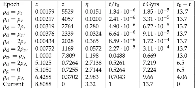
Table 1. Epochs of equality of densities and forces.
Epoch x z η t/t0 tGyrs t0−t
ρd=ρr 0.00159 5529 0.0151 1.34·10−6 1.85·10−5 13, 7 ρd=ρν 0.00217 4057 0.0200 2.41·10−6 3.31·10−5 13.7 ρd=2ρr 0.00319 2764 0.280 4.90·10−6 6.72·10−5 13.7 ρd=ρrν 0.00376 2339 0.0324 6.64·10−6 9.11·10−5 13.7 ρd=2ρν 0.00434 2028 0.365 8.59·10−6 1.72·10−4 13.7 ρd=2ρrν 0.00752 1169 0.0572 2.27·10−5 3.11·10−4 13.7 ρrν=ρΛ 1.0000 7.809 1.198 0.0488 0.669 13.0 ρd=2ρΛ 5.1025 0.7264 2.7138 0.5261 7.219 6.5 ρg=0 5.1050 0.7255 2.7144 0.5264 7.224 6.5 ρd=ρΛ 6.4288 0.3702 2.983 0.7043 9.66 4.06
Current 8.8088 0 3.32 1 13.7 0
4.3. Roles of components at different epochs 291
In the expressions for total mass density
ρt=ρc=ρd+ρrν+ρΛ=ρ0cΩ0Λ1+βx+x 4
x4 (44)
and gravitational mass density
ρg =ρd+2ρrν−2ρΛ=ρ0cΩ0Λ2+βx−2x 4
x4 (45)
the mass density of dark energy is constant, while others decrease with time. Therefore, at different 292
epochs the components have played different roles. 293
At certain points in time, the densities become equal. Since the components give different 294
contributions to the gravitational mass density — the radiation gives a double positive contribution, 295
and the vacuum gives a double negative one — their effect on the gravitation is different at different 296
times. All of these moments are given in Table 1, which lists the values of the parameterx, the redshift 297
z, and the coordinateη, the fraction of the full age and the age of the universe itself at the corresponding 298
moments, as well as the time elapsed from these moments to the present epoch. The gravitational mass 299
density becomes zero at a value ofxdetermined by the equationx4−(β/2)x−1=0. Moments when 300
ρd=ρΛand whenρg=0 almost coincide, because the radiation and neutrino densities are small at 301
these moments. The moment whenρrν=ρΛcorresponds to the time whenxis very close to 1.
302
4.4. Distances, speeds, acceleration: past, current, and future 303
In the flat model, sn0(χ) = χ, the quasicenter and real center of spheres coincide, the parallax distance and the radius of a sphere are equal to the metric distance:lpl=r=l. In the Standard model the expressions forl/l0Hand the dimensionless velocity of the expansionv/ccoincide as well. Indeed, at any moment:
v c =
˙ l c =
H cl=
l
lH. (46)
In the Standard model the metric distance from the observer in the current universe to a location with coordinateχis given by the formula following from (26) and (38):
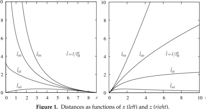
˜
lnb ˜lbb ˜l=l/l0H ˜lbb ˜lnb ˜l=l/l0H
˜
lpl ˜lpl
˜
lad ˜lad
x z
10
8
6
4
2
0
0 2 4 6 8 10
0 0 2 4 6 8 10
1 2 3 4 5 6 7 8
Figure 1. Distances as functions ofx(left) andz(right).
Table 2. Epochs associated with the characteristic values of redshift.
x z η t/t0 tGyrs t0−t
0.0088000 1000 0.064629 2.9659·10−5 4.0697·10−4 13.721 0.017582 500 0.10796 9.4743·10−5 1.3000·10−3 13.720 0.087215 100 0.30606 1.2021·10−3 0.016494 13.705 0.17272 50 0.45696 3.4279·10−3 0.047036 13.675
0.80080 10 1.0642 0.034925 0.47924 13.242
0.97875 8 1.1841 0.047233 0.64811 13.074
3.3491 1.6302 2.2320 0.29360 4.0288 9.6930
3.6350 1.4233 2.3224 0.33008 4.5293 9.1925
2.2022 3 1.8084 0.15891 2.1806 0.11541
The equalities (25) can be rewritten as
lbb0 =l0nb√1+z=l0pl(1+z) =lad0 (1+z)2=R
0χ(1+z) =l0(1+z). (48) In what follows, we refer mainly to current values and use dimensionless distances, measuring them in terms of the Hubble distance according to the scheme ˜l=l/lH0. Therefore, all distances are expressed (asv/cin (46)) via the metric distance:
˜ lpl=
v
c =l˜=η∗[I0(x0,β)−I0(x,β)], l˜ad=la,˜ l˜nb= ˜ l
√
a, l˜bb= ˜ l a, a=
x x0
= 1
1+z. (49) Figure1plots dependences of distances on the variablex(left) and redshiftz(right).
304
Let us consider three additional moments in time corresponding to particular events. The first 305
event was the phisical horizon (aboutz=1000), the second was when the angular size distance had its 306
maximum value (z=1.6302), and the third was when the current metric distance equaled the Hubble 307
distance (z=1.4233). These data, and also for comparison, the moments corresponding to several 308
characteristic values of redshift, are given in Table 2, serving as a continuation of Table 1. Table 3 309
lists the values of the distances to the points indicated in Tables 1 and 2. The rate of change of the 310
parallactic distance coincides withv/c, since this distance corresponds to the metric distance. The 311
rates of recession of the remaining distances are determined from their definitions by differentiation 312
with respect to time while keeping the spatial coordinateχfixed. The expressions for these velocities 313
Table 3. Distances to characteristic points of the Standard Model.
z l˜ l˜ad l˜nb l˜bb
∞ 3.322 0 ∞ ∞
5529 3.307 5.981·10−4 245.9 18288 4057 3.302 8.138·10−4 210.4 13401 2764 3.294 1.192·10−3 173.2 9108 2339 3.290 1.406·10−3 159.2 7700 2028 3.286 1.619·10−3 148.0 6667 1169 3.265 2.790·10−3 111.7 3821 1000 3.258 3.255·10−3 103.1 3261 500 3.214 6.416·10−3 71.95 1610 100 3.016 0.02987 30.31 304.7 50 2.865 0.05619 20.46 146.1
10 2.258 0.2053 7.490 24.83
8 2.138 0.2376 6.415 19.25
7.809 2.125 0.2412 6.306 18.72
3 1.514 0.3785 3.028 6.056
1.630 1.090 0.4146 1.768 2.868 1.423 1.000 0.4126 1.557 2.423 0.7264 0.6086 0.3525 0.7996 1.051 0.7255 0.6100 0.3524 0.7987 1.049 0.3702 0.3397 0.2479 0.3977 0.4655
0 0 0 0 0
Table 4. Current velocities of recession at different distances.
Metric ad pl nb bb
H0l H(η0−χ)lad H0lpl
3H0−H(η0−χ)
The acceleration of the cosmological expansion is determined by the first equation in (12):
˙
v=l¨= d
2
dt2l 0
Haχ=lH0a¨χ= ¨ a al=−
4πG
3 ρgl =H 2 Λx
4−
βx/2−1
x4 l. (50)
As already mentioned, in the gravitational mass density ρg = ρd+2ρr−2ρΛdensitiesρdandρr decrease with increasing age of the universe, whileρΛ = ρ0Λ. Therefore, in the numerator of the last fraction in (50), the relative importance of the first term increases with time. At the present time (x=x0), the gravitational mass density is negative:ρ0g=ρ0d+2ρ0r−2ρ0Λ=−1.0677·10−29 g/cm3, so that the expansion occurs with an acceleration. But the acceleration at the current Hubble distance (speed equal to the speed of light) is only
˙
v0H =−4πG
3 ρ 0 glH0 =
H0c 2 (2Ω
0
Λ−Ω0d−2Ω0rν) =3.94·10−
8 cm/s2≈4 A◦/s2. (51)
In the distant future att→∞(η∞=4.4514)
a= 1
1+z ∼ Ω0
d 4Ω0 Λ
!1/3
eHΛt=0.46000eHΛt, x∼4.0520eHΛt,
η∼η∞−2.5619e−HΛt. (52)
Thus, the scale of the universe will increase exponentially, so that a second inflation will take place, 315
which we will discuss in more detail later. However, according to (52), an exponential expansion 316
will really begin only at t ∼ tΛ = 1/HΛ. The time scale is 1/H0 = 4.4081·1017s= 13.969 Gyr, 317
tΛ = 1/HΛ = 5.1950·1017 s= 16.462 Gyr. We also define the distancelΛ = c/HΛ = l0 H/
q Ω0
Λ = 318
1.5574·1028cm=5.0473 Gpc. 319
The speed of expansion of space at the Hubble distance is, by definition, equal to the speed of light. The velocity of recession of the Hubble distance is derived using equation (15):
˙ lH = d
dt c H =−
c H2H˙ =
c H2
H2+4πG
3 ρg
=c
1+1
2 ρg
ρc
= c
2
4+3βx
1+βx+x4. (53) According to this formula, at the beginning of the expansion the velocity is close to the two speeds of light, decreasing with time, and in the distant future it will approach zero. Acceleration at the Hubble distance increases with time, but remains finite:
˙
vH =−4πG
3 ρglH=− 4πG
3 ρg c
H = HΛc
x4−βx/2−1 x2p
1+βx+x4 →
HΛc=5.77A ◦
/s2. (54)
Acceleration of the distance itself is negative:
¨ lH =−c
2 HΛ
x
β+16x3+9βx4
(1+βx+x4)3/2 ∼ −cHΛ 9 2
β
x3. (55)
From these formulas it is clear that the accelerations are of the same order as the product of the 320
speed of light and the current Hubble constant, or the asymptotic value of the Hubble parameter: 321
cH0 =3·1010·2.27·10−18 =6.81·10−8cm/s2,cHΛ=5.77·10−8cm/s2(which coincides with the 322
limit of (54)). 323
4.5. Evolution of redshift and apparent luminosity 324
As mentioned above, the scale factora, and therefore the redshift 1+z = 1/aare tied to the 325
epoch of observation. Therefore, the value ofzfor each sufficiently distant object should change with 326
increasing age of the universe. Therefore, luminosities of objects should change as well. A. Sandage 327
ofΩ0d([36]). In the Appendix [37] to the paper [36], McVittie made the same calculations while adding 329
a cosmological term. Later A.Loeb [38] (apparently independently) proposed to determine changes in 330
the redshiftzof quasars using observations of theLα-forest with the 10-meter Keck telescope. He also
331
transformed these changes into changes of the velocities of radiating objects. Such changes are known 332
as the Sandage-Loeb effect. 333
Let us find the dependence of the change ofzon the age of the universe according to the Standard 334
model. Since for this relation the dependence of the radius of curvature on time is significant, we 335
will writeR(t)without changing the notation. The redshift of lines in the spectrum of some object 336
at a location corresponding to timet= t(η)from the beginning of the expansion, and observed at 337
a position corresponding to the fixed timet0 = t(η0), is determined by the well known formula 338
1+z= R(t0)/R(t). Thenzis uniquely related to timet, and equal to 0 at the observer’s location, 339
z = 0. For the complete definition ofz, both times should be specified as arguments, i.e., z(t,t0). 340
However, this is traditionally not done, since the epoch oft0is fixed; in the pastz>0 and in the future 341
−1<z<0 with respect tot0. At this point we adopt a more detailed designation. 342
After some time has passed, the age of the universe has increased and the epoch to which redshifts are attached has moved to the momentt00=t(η00). Then an object at a given redshift has moved to time t0 =t(η0)without changing its spatial coordinateχ. A connection between the moments of emission of radiation and its reception by the observer does not change in terms of the conformal coordinates, and the difference between the times of the observer and the object is preserved:
χ=η00 −η0=η0−η, η00 −η0=η0−η. (56)
In particular, the infinitesimal displacements are equal as well: dη0 =dη. Using the relationcdt= R(t)dηat timestandt0, we obtain the relation between the differentials of time and the derivative of one with respect to the other:
dt0= R(t0)
c dη0= R(t0)
c dη= R(t0)
c c R(t)dt=
R(t0)
R(t)dt,
dt dt0 =
R(t)
R(t0) =
1
1+z. (57) The last relation between the passage of time of the object and the observer has already been used in 343
section3.5for the transformation from a parallactic distance to a distance measured according to the 344
flux of photons. 345
To detect changes ofz, one must measure shifts of lines in the spectrum of a source (with the same value of theχcoordinate) at different times. The difference between the times should be much smaller than the times themselves, so increments of values can be replaced by their differentials (infinitesimally small), and it is sufficient to determine the derivatives of the variables. Using (57) we find:
dR(t)
dt0 = dR(t)
dt dt
dt0 =R˙(t) R(t)
R(t0),
dR(t0)
dt0 =R˙(t0). (58) From the latter we obtain ([36])
dz dt0
= d(1+z)
dt0
= d
dt0 R(t0)
R(t) =
˙ R(t0)
R(t) −
R(t0)
R2(t)R˙(t) R(t)
R(t0)
= R˙(t0)
R(t0) R(t0)
R(t) −
˙ R(t)
R(t) = H0(1+z)−H.
(59) The dependence ofHonzis derived ifxis substituted byx0/(1+z)in (37).
346
A change in the redshift will result in a change in the observed luminosity of objects. The rate of change of the photometric distance in the current epoch, as follows from the equalities (24), (48) (its boundary partslbb0 =l0(1+z)) and (59), is equal (in accordance with Table 4) to:
dlbb0 dt0 =l˙
0(1+z) +l0dz dt0 = H0l
0(1+z) +l0[H
0(1+z)−H] =
2H0− H 1+z
Then
˙
L0bb=−2 LO 4π(l0bb)3
dl0bb dt0 =−2
L0bb lbb0
dlbb0 dt0 =−2L
0 bb
2H0−
H 1+z
, 1
H0
d lnL0bb dt0 =−2
2− 1
1+z H H0
. (61)
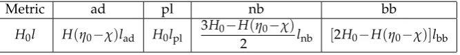
Figure2(for brevity, the derivative dz/dt0is denoted by ˙z) presents the dependencies of ˙z/H0 347
and ratio ˙z/[H0(1+z)]on the (current) redshiftz. First, the speed ˙zis positive, i.e.,zincreases; at 348
z=2.34 the derivative ˙zbecomes zero. Between two zeros (atz=0 andz=2.34) at the pointz=1.06 349
there is a maximum equal to 0.280. The redshifts of more distant objects (z>2.34) decrease; moreover, 350
the rate of decrease grows rapidly with recession (increasingz): ˙z/H0is equal to−0.98,−1.8,−8.4, 351
−30 atz=4, 5, 10, 20 respectively. For the ratio ˙z/[H0(1+z)], the growth is less pronounced. The 352
derivatives ˙zand ˙z/(1+z)are equal to zero at the same points, and ˙z/(1+z)reaches the maximum 353
atz=0.726 that is smaller than the maximum of ˙z. 354
Figure2also presents a graph of the dimensionless derivative of the logarithm of the apparent 355
luminosity as a function ofz. Whenz=0 this derivative equals−2, which reflects a decrease in the 356
solid angle of the source at the very beginning of the source’s recession from the observer. At smallz 357
the rate of decrease grows slightly; atz=0.726 it has maximum negative value, then decreases and 358
becomes equal to zero atz= 13.2. The apparent brightness of distant objects should increase with 359
redshift atz >13.2. The effect is stronger for more distant objects, although it is unclear whether 360
any radiating objects existed, since such redshifts correspond to times<326 million years from the 361
beginning of the expansion, less than a fraction 0.0238 of the current age of the universe. 362
˙
z H0
1
H0 ˙
z
1 +z
1
H0 d lnL0
bb dt
z
0 2
0.5
0.0
−0.5
−1.0
−1.5
−2.0
−2.5
4 6 8 10 12 14
Figure 2. Changes in redshift and luminosity as a function ofz.
It is most convenient to measure changes in all of these quantities when observing theLα-forest,
363
which corresponds to shifts of theLαline in the spectra of distant quasars due to gas clouds located
364
along the path to them. These clouds can have peculiar radial velocities relative to the Hubble flow 365
that can affect observed shifts of the line. However, values of these radial components most likely 366
do not change significantly during the time between observations if they are separated within some 367
decades up to hundred of years. The luminosities of objects do not change as well at least in average. 368
Despite the importance of this effect to test the theory, any possibility of observing it with modern instruments would require a very long time interval between observations, from hundreds to thousands years, sinceλ(t0)/λ(t) =1+z(t,t0), then dλ0/λ0=dz/(1+z), and
dt0= 1
H0
dz/(1+z)
˙
z/[H0(1+z)]. (62)
For example, if we assume that the accuracy of measurements of a relative shift of lines is dλ/λ= 369
10−6/0.2=3·103yrs — a time interval which is insignificant on cosmological scales but longer than 371
a human lifetime. For largez, the accuracy of measuring the position of the lines is less, so that we 372
would need major technological progress to pursue such a method. 373
[39] estimates the possibility to detect the shift of lines due to cosmological expansion in the 374
spectra of various objects at different wavelengths for different cosmological models when telescopes 375
with ultra-large mirrors (40–60 m) become available, as is planned for the 2020s. It is alleged that a 376
42-m telescope will be able to measure the shift with 4000 hour exposures separated by 40 yrs. The 377
article also provides an overview of previous work on the question of changing redshift. 378
5. The second inflation and the second horizon 379
5.1. Visible and invisible parts of the universe 380
According to the theory of cosmological inflation, near the very beginning of the evolution of the 381
universe, space expanded exponentially. The standard theory, as follows from (52), predicts that a 382
positive cosmological constant causes an acceleration of space starting from a certain moment that 383
leads to an exponential expansion, although at a much lower rate than during the first inflation. This 384
new expansion generates a new concept: a second horizon. 385
The equation of motion of a photon traveling to the observer (that is, to us) is χ = η0−η; therefore, the place and time of its exit are related by the equalityχe=η0−ηe<η0. So, the equation of motion can be rewritten as follows:χ=χe+ηe−η. Therefore, the distance from the observer to the approaching photon is
lrs =l0Ha(η)(χe+ηe−η). (63) The parameter η is limited. Fort = ∞, it is equal to η∞ = 4.4514. The distance can only equal 386
zero,lrs = 0, ifχe+ηe < η∞. Then there is another limitation on the ability to observe objects in 387
the universe: along with the first horizon there is a second one. The concept of two horizons was 388
introduced by V. Rindler [40] and discussed in a number of papers, for example, in [41]. Here their 389
kinematic characteristics are derived within the Standard model. 390
The first horizon is called geometric (we recall that the physical horizon is the sphere of last 391
scattering atz ≈ 1000), while the second horizon can be called the kinematic or dynamic horizon. 392
Other names are also used, borrowed from the terminology of the theory of black holes. The geometric 393
horizon is called the particle horizon, and the kinematic horizon is called the event horizon. These 394
names were introduced by Rindler. 395
At an arbitrary epoch,η, the first and second horizons are determined by the equations
χGHor=η=H0
a
Z 0
da
a2H =η∗I0(x,β), χKHor=η∞−η=H0 ∞ Z
a
da
a2H =η∗[I0(∞,β)−I0(x,β)]. (64)
In Figure 3 positions of the geometric horizon are indicated on the ordinate axis. The lines 396
corresponding to this horizon are parallel to the abscissa. They rise with time, reflecting expansion of 397
the horizon. The second, kinematic horizon is shown by a straight line connecting the abscissa and 398
the ordinate, which are equal toη∞, while its specific position corresponds to the time on the abscissa 399
axis. The paths of photons coming toward us are represented by straight lines parallel to this straight 400
line. Photons can start their journey from any point on the trajectory. Photons, for whichηe+χe<η∞, 401
that is, moving along straight lines lying below the straight line specified above, sooner or later will 402
reach a place where the observer is located. For example, Figure3shows the paths of photons that 403
have reached our position at timeη∗<η0and at the current epochη0. Ifηe+χe>η∞, then photons 404
with such coordinates never reach our location. According to the equalityηe+χe=η∞, it would seem 405
takes some additional vertical space
χ
eη
1η
∞η
0η
∗η
∗η
0η
∞η
eFigure 3. Visible and invisible parts of the universe.
From behind the first horizon, the radiation has not yet reached the observer. The second horizon 407
separates the region of times and locations from which radiation cannot reach the observer, since the 408
photons coming from there are moving away from the observer. This occurs because space expands at 409
speeds higher than the speed of light, and these speeds increase with time. At the current time, we can 410
see objects in the universe up to redshiftsz≈10, but this corresponds to the past. We will never see 411
objects located now at redshiftsz≥1.725. 412
Indeed, if a photon is now emitted toward us from a place with coordinateχo, then the distance 413
to it at momentη will be lph = l0Ha(η)(χo+η0−η). This distance can become equal to zero at 414
η = χo+η0, and it must be the case thatχo+η0 < η∞. Thus, the boundary of the coordinateχo 415
for photons emitted now isχ0lim = η∞−η0 = 1.13. The values of x0lim = 3.23, z0lim = 1.725, and 416
llim0 =4.84 Gpc=lKHor0 correspond to this coordinate. The sphere of such a radius is the current second 417
horizon. Thus, the radiation from the points now located at distances of 4.84 Gpc from us will never 418
reach us, even in the infinitely remote future. Figure4shows distanceslrsto the photons arriving 419
at the observer at the epoch whenη =2 (Figure4left), and at the current epoch (Figure4right). In 420
Figure5these distances are given as a function of values ofxfor cases where the sum of the coordinates 421
of time and location of the photon emission is equal toη∞(Figure5left) and larger than that (Figure5 422
right). These figures also show curves reflecting the relationship between the timeηeand the location
423
χeof the photon emission.
424
Generally speaking, if a photon is emitted at a point where the expansion speed is greater than 425
the speed of light, this does not necessarily mean that it will not reach us. Cosmological expansion 426
occurs in the same way with respect to all points of space, and it starts after a period of inflation with a 427
very high speed (formally infinite, according to formula (37), which defines the Big Bang), although in 428
the beginning the expansion was slowing down. A photon emitted from far away, where the speed 429
of expansion is large but closer than the horizon, still comes to us, because it gradually moves into 430
layers of space expanding at a slower and slower rate. At some point its velocity toward us becomes 431
zero, and then becomes negative, that is, it begins to approach us. However, it takes a long time for the 432
photon to reach us. Consider, for example, a galaxy observed by us now at redshiftz=3: according to 433
Table 2, it moves away from us with a speed ofH0l=cl˜=1.51c, and earlier its speed was greater. At 434
/
takes some additional vertical space
ηe+χe= 2 ηe+χe=η0
χe
ηe ηe χe
˜
lrs
˜
lrs
x x
1.5
1.0 2.5
0.0 0.5 2.0
1.5
1.0 2.0
0.5
0.0 0.0
0.5 1.0 1.5 2.0 2.5 3.0 3.5
0 1 2 3 4 5 6 7 8
Figure 4. The paths of photons with arrival time at epochs:η=2 (left) andη0=3.3224 (right).
space
ηe+χe=η∞ ηe+χe= 5
ηe
χe
ηe
χe
˜
lrs
˜
lrs
x x
0 10 20 30 40 50
0 1 2 3 4 5
0 6
1 2 3 4 5 7
0 20 40 60 80 100
the distant past, when neither the Earth, nor even the Sun, existed (but the galaxies and stars of the 436
previous generations had already formed). 437
Figure4shows that the distance of a photon emitted sufficiently early at first increases, which 438
means expansion with a speed greater than the speed of light, faster than the photon speed. From the 439
point where the distance reaches a maximum, the photon begins to approach and finally arrives at our 440
location. However, as shown in Figure5, this is not possible ifηe+χe≥η∞, even if the equality is true. 441
Figure5leftshows that a photon emitted at the second horizon, and which then travels along it, would 442
not arrive at the observer after an infinite time; in fact, the photon only recedes along with the horizon. 443
After an infinite time, such a photon will be at a distancelΛ≈5.0 Gpc, since the factorη∞−ηin the 444
formula (63) atχe+ηe = η∞tends to zero ift→ ∞, while the factora(η) →∞, but their product 445
remains finite. A photon emitted atηe+χe<η∞may, after a very long time, reach the current location 446
of our civilization, but one emitted atηe+χe>η∞will only recede from us, eventually exponentially 447
fast. The reason for this is the accelerated expansion of space. Thus, galaxies located on the second 448
horizon and behind it will forever disappear from our field of view. These statements follow from the 449
formulas given below. 450
5.2. Distances, velocities, and accelerations of horizons 451
Distances to horizons at an arbitrary epochη according to equations (64) are defined by the 452
formulas: 453
lGHor=l0Ha(η)η=lΛxI0(x,β), (65) lKHor=lH0a(η)(η∞−η) =lΛx[I0(∞,β)−I0(x,β)]. (66) The sum of the horizon conformal space coordinates is constant at all times, and the sum of the 454
distances to them is proportional to the scale factor. Both horizons expand. The speed of the geometric 455
horizon exceeds by the speed of light the velocity of the position where the horizon is located at time 456
˙
lGHor=lH0a˙η+l0Haη˙=HlGHor+c. It expands at an accelerating rate. In contrast, the velocity of the 457
kinematic horizon is less than the speed of its location by the speed of light: ˙lKHor =l0Ha˙(η∞−η)− 458
l0
Haη˙ =HlKHor−c, and its expansion slows down. 459
Asymptotes of distances to horizons and their velocities att→∞,a→∞,z→ −1 are determined 460
by taking into consideration thatI0(∞,β) =0.42880 andI0(∞,β)−I0(x,β)∼ 1 x
1−18xβ3
: 461
lGHor∼l0Hη∗I0(∞,β)a=5.9·1028acm∼2.7·1028eHΛtcm→∞, (67) lKHor →
c
HΛ =1.56·10
28 cm=5.05 Gpc. (68)
The current distance to the geometric horizon islGHor0 =lH0η0=3.32l0H=4.39·1028cm=14.2 Gpc. 462
The velocity near the horizon isv0GHor=cη0=3.32c, and the velocity of the expansion of the horizon 463
is ˙l0GHor=4.32c. The horizon will cross 4.32 light years in one year, which is equal to 1.33 pc, so that 464
1 Gpc will be added to the current 14.2 Gpc in 0.755·109years if the speed of the horizon is equal to its 465
current velocity, and in 0.741·109years if the increase of the velocity is taken into account. 466
The current distance to the second horizon isl0KHor=lH0(η∞−η0) =1.49·1028cm=4.84 Gpc. The 467
limit to this distance coincides with the Hubble limit:lKHor→ l
0 H q
Ω0 Λ
= c
HΛ =5.05 Gpc. The current 468
speed of expansion of the location of this horizon isc(η∞−η0) =1.13c, and the speed of recession of 469