Modeling and Detection of Future Cyber-Enabled DSM Data Attacks

Article

Modeling and Detection of Future Cyber-Enabled

DSM Data Attacks

Kostas Hatalis1, Chengbo Zhao2, Parv Venkitasubramaniam3, Larry Snyder4, Shalinee Kishore 5_{and Rick S. Blum}6

1 _{Dept. of Electrical and Computer Engineering, Lehigh University, Bethlehem, PA, 18015, USA;}

[email protected]

2 _{Dept. of Electrical and Computer Engineering, Lehigh University, Bethlehem, PA, 18015, USA;}

[email protected]

3 _{Faculty of Electrical and Computer Engineering, Lehigh University, Bethlehem, PA, 18015, USA;}

[email protected]

4 _{Faculty of Industrial and Systems Engineering, Lehigh University, Bethlehem, PA, 18015, USA;}

[email protected]

5 _{Faculty of Electrical and Computer Engineering, Lehigh University, Bethlehem, PA, 18015, USA;}

[email protected]

6 _{Faculty of Electrical and Computer Engineering, Lehigh University, Bethlehem, PA, 18015, USA;}

[email protected]

Abstract:Demand-Side Management (DSM) is an essential tool to ensure power system reliability and stability. In future smart grids, certain portions of a customer’s load usage could be under the automatic control of a cyber-enabled DSM program, which selectively schedules loads as a function of electricity prices to improve power balance and grid stability. In this scenario, the security of DSM cyberinfrastructure will be critical as advanced metering infrastructure and communication systems are susceptible to cyber-attacks. Such attacks, in the form of false data injections, can manipulate customer load profiles and cause metering chaos and energy losses in the grid. The feedback mechanism between load management on the consumer side and dynamic price schemes employed by independent system operators can further exacerbate attacks. To study how this feedback mechanism may worsen attacks in future cyber-enabled DSM programs, we propose a novel mathematical framework for (i) modeling the nonlinear relationship between load management and real-time pricing, (ii) simulating residential load data and prices, (iii) creating cyber-attacks, and (iv) detecting said attacks. In this framework, we first develop time-series forecasts to model load demand and use them as inputs to an elasticity model for the price-demand relationship in the DSM loop. This work then investigates the behavior of such a feedback loop under intentional cyber-attacks. We simulate and examine load-price data under different DSM-participation levels with three types of random additive attacks: ramp, sudden, and point attacks. We conduct two investigations for the detection of DSM attacks. The first studies a supervised learning approach, with various classification models, and the second studies the performance of parametric and nonparametric change point detectors. Results conclude that higher amounts of DSM participation can exacerbate ramp and sudden attacks leading to better detection of such attacks, especially with supervised learning classifiers. We also find that nonparametric detection outperforms parametric for smaller user pools, and random point attacks are the hardest to detect with any method.

Keywords: Demand Side Management, Demand Response, Cyber-Physical Systems, Dynamic Pricing, Load Forecasting, Attack Detection

1. Introduction

Demand-Side Management (DSM) is an essential component in smart grids for planning, monitoring, and modifying consumer load levels. Furthermore, cyber-enabled DSM will allow smart grids even higher levels of automated decision-making capabilities to selectively schedule loads on local grids to improve power balance and grid stability. Such a cyber approach relies heavily on real-time, two-way communication capabilities between a central controller and various adaptable loads. Research into the reliability of the cyberinfrastructure that enables DSM is therefore vital. The main concerns in ensuring DSM security lay in the feedback mechanism of real-time electricity pricing and distributed DSM controllable loads. For instance, in residential grids, a single home consumes only a small amount of electric power, and if it becomes compromised, then it might not have a noticeable impact on the power grid. However, a carefully planned or even random cyber attack might impact other loads not under attack by taking advantage of the feedback mechanism of load management.

Two-way communication capabilities of Advanced Metering Infrastructure (AMI) enables a utility or Independent System Operator (ISO), in the retail power markets, to collect high-resolution energy

usage from consumers and enable dynamic pricing to adapt to consumer demand [1]. AMIs provide

an efficient way for ISOs to schedule prices and then communicate them to consumers for automatic DSM control of certain portions of a consumer’s load. AMIs can also provide practical ways for ISOs to set DSM goals, such as reducing peak or decreasing aggregate load levels through price influences. However, there are several vulnerabilities in AMIs that present noteworthy security issues since they

are directly accessible by users [2]. Due to the large scale deployments of AMIs, ISOs encourage the

utilization of marginally cheaper hardware, resulting in constrained computational resources to allow for robust security capacities, such as intrusion monitoring.

DSM programs also utilize demand response, a specific tariff or program to motivate customers to respond to changes in price or electricity availability over time by altering their regular electricity

use habits. We take this a step further and look at future cyber-enabled DSM programs [3] that

will autonomously control household loads such as water heaters and HVAC units based on Real Time Pricing (RTP). As part of the reliable implementation of this future cyber-DSM, it is crucial to understand the dependency between dynamic pricing and automatic demand response as well as the risks. We hypothesize that cyber-DSM programs can be particularly vulnerable to cyber attacks such as false pricing information or direct load manipulation, especially when the participation rate in DSM is high.

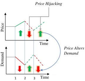
Our work is thus motivated to study these vulnerabilities in DSM. We provide a mathematical formulation of the feedback between utilities and DSM systems, and then simulate, analyze, and test different detection methods for attacks on such feedback. This relationship between load and price

is shown visually in Fig.1. As prices go up, demand naturally responds by decreasing. However, if

AMIs are hijacked, and false lower prices are reported to DSM systems, there will be an inappropriate increase in demand. A similar effect happens if an attacker directly controls user loads. Then a higher load usage by the attacker may inadvertently lead to higher prices for the rest of the grid. We present a standard of how attackers can exploit such a dependency.

We propose a mathematical framework of the feedback between price setting and DSM systems to study how attacks can be structured and how to detect them. Similar frameworks have been considered

in previous work. In [4], the author applied a profitable attacking strategy to a price-load dependency

model. Another control-theoretic approach to derive the fundamental conditions of Real Rime Pricing

(RTP) stability under integrity attacks is described in [5]. The authors in that work use an elasticity

model between price and load and apply an autoregressive model to obtain the forecast load and price. The main contributions of our approach can be summarized as follows:

De

mand

Time

P

ric

e

Time

1

2

3

Price Hijacking

Price Alters

Demand

Figure 1.Feedback effect between price and DSM demand. As prices go up, demand decreases. But if prices are hijacked and false prices are fed to DSM systems then a false low price increases demand, and a false high price can decrease demand. The same is true if demand was altered by an attack. If load usage is increased by an attacker then prices would increase and vice versa.

2. We propose two modes of attacks on DSM systems: false pricing data injection and direct load manipulation. We prove their equivalence and highlight three types of attacks that could be undertaken by each mode. We then empirically show how an increased use of DSM can exacerbate attacks.

3. We simulate these attacks and compare sequential change-point and machine learning methods, as well as a deeper dive in parametric vs nonparametric methods, for detecting DSM attacks. In our main results, we demonstrate the impact of DSM on detection performance and identify what kind of detectors are effective for different attacks.

In Section2, we provide a literature review on DSM and important DSM strategies on real-time

pricing and load forecasting. In Section3we present a block bootstrap technique for simulating the

non-DSM load distribution of a micro-grid ofNhomes from template residential load time series. We

then propose dependency models for the feedback nature of load and prices in Section4, where we

also showcase simulations of residential load and electricity prices when an automatic DSM program

controls certain portions of consumer demand as a function of price. In Section5, we present two

modes of cyber attacks, direct load manipulation attacks, and price data injection attacks that can have a significant influence on the feedback of load and price. We prove these two attacks are equivalent. In

Section6, we review several sequential detection and supervised learning methods. In Section7we

present our experimental result compare performance under different DSM participation rates when they are under three types of attacks: ramp, sudden, and point attacks. We find that point attacks are hardest to detect, and supervised learning methods can provide better results than sequential detection methods. To provide a deeper analysis, we also conduct a comparison of parametric and

2. Background

2.1. Demand Side Management

DSM is an active and voluntary approach for reducing electricity use through activities or programs that promote electric energy efficiency, conservation, or more efficient management of

electric energy loads [6]. Very often, ISO’s utilize financial incentives and educational programs to

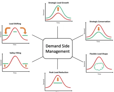
modify consumer demand. The main goals of DSM are peak clipping, valley filling, load shifting, strategic load growth, flexible load shaping, and strategic conservation. We summarize these goals in

Fig. 2. In these goals, consumers are encouraged to use less energy during peak hours, or to move

the time of energy use to off-peak times such as nighttime, or reduce overall consumption. Other applications for DSM are to aid grid operators in balancing intermittent generation from wind and solar farms due to their volatile nature, which may not coincide with energy demand at different times.

Our study focuses on modeling and simulating the DSM goal of strategic conservation due to its simplicity and essential use in the smart grid. This goal also makes it easier to study attacks on DSM by modeling strategic conservation as a general reduction in load. Attacks then could stand out more visibly then under other goal schemes like flexible load shaping. More specifically, this DSM goal aims at reducing aggregate load demand through directed reduction of electricity consumption. The successful implementation of strategic conservation programs usually requires some combination of financial incentives to customers, energy-efficient building standards, and appliance efficiency improvement. We envision that AMI and smart appliances in residential DSM programs will automatically control specific portions of consumer load as a function of real-time electricity prices to achieve the goal of strategic conservation.

Most DSM programs are formulated as an optimization problem as follows

min

Pt

T

∑

(Lt−L0t)2,

wherePtis the RTP at timet,Ltis actual load, andL0tis the target load level the ISO is interested in

achieving via DSM. The aim is to choose a pricePtfor each time step such that the actual load would

reach as close as possible to the target level. In [7], a DSM strategy is proposed based on a heuristic

optimization strategy to shape the load curve close to the desired shape. A heuristic-based evolutionary algorithm was used to solve the above minimization problem. A multi-agent game-theoretical DSM

approach is proposed in [8]. The authors use game theory and formulate an energy consumption

scheduling game, where the players are the users, and their strategies are the daily schedules of their

household appliances and loads. In [9], the minimization problem is solved by utilizing a feedforward

neural network to map the nonlinear relationship between price and load. Recently, the DSM problem

is addressed in [10] as a multi-objective optimization problem that also seeks to balance other merit

Deman

d

Flexible Load Shape

Time

Strategic Load Growth

Deman

d

Time

Time

Strategic Conservation

Deman

d

Time

Peak Load Reduction

Deman

d

Time

Valley Filling

Deman

d

Time

Load Shifting

Deman

d

Demand Side

Management

Figure 2.Various demand side management goals.

2.2. Load Forecasting

Load Forecasting (LF) techniques are essential for RTP and other ISO operations by predicting future energy requirements of a system from previous data and weather conditions. It is recognized as the initial building block of utility planning efforts and ensures the balance between supply and demand of energy, LF thus plays a vital role in our DSM formulations. For a given system and requirements, LF provides predictions for specific periods. These periods are divided into short, medium, and long term forecasts. Short term LF is used to predict the load on an hourly basis for up to 1 week when considering daily operations and cost minimization. Medium-term LF typically predicts load on a weekly, monthly, or yearly basis for efficient operational preparations. Long term LF is used to predict the decades’ load to facilitate grid and generation expansion planning. In this work, we look at short term LF to predict loads from one hour to a week.

LF models can be divided into two approaches [3], the first being statistical based modeling

and the second being machine learning. The statistical approach can be further broken down into regression and time series models. Multiple linear regression can be used with the weighted least squares estimation technique to form a relationship between different independent covariates when load depends on such things as weather conditions. Regression models have been applied in LF

in different works, such as in [11]. Time series models are also prevalent to apply to LF. The most

common model is the AutoRegressive Moving Average (ARMA) model and its variants that include components such as integration (I), Fractional Integration (FI), multiVariate series (V), Seasonality (S), eXogenous (X) data, Conditional Heteroskedasticity (CH), and Nonlinearity (N). For our formulation, we employ SARIMA for LF.

Hyperparameters of ARMA models can be configured using Box-Jenkins decomposition or grid-search with the Akaike information criterion. Numerous studies have looked at all the different

ARMA models for LF [12]. Other time series methods for LF include simple exponential smoothing

many models and ideas, but they are theoretically different. Time series analysis first deals with time-indexed stationary data and accounts for the autocorrelation between time events. In regression, we assume there is no autocorrelation, and that all observations are independent and identically distributed. Furthermore, we also assume that in regression, the data is homeostatic and does not exhibit multicollinearity.

Most recently, machine learning methods have seen a huge spike in LF research. Machine learning models are data-driven, typically providing a nonlinear fit to input covariate data to predict load. The advantages of this approach include not needing preconditions for data such as stationarity (a requirement for most time series methods), excels at modeling nonlinear dependencies, and can fit large data sets. Disadvantages for most machine learning models are that most hyperparameters are continuous (difficult to tune), they require extensive feature engineering, and may get stuck in local

minimums. Models for LF include support vector machines [15], feedforward neural networks [16],

recurrent neural networks [17], random forests [18], and ensemble learning [19].

2.3. Real Time Pricing

Every consumer of electricity is charged a certain amount per kiloWatt-hour (kWh) of energy. Such a charge covers the costs associated with the generation, transmission, and distribution of electricity. The two main types of costs are operational and fixed costs. During the 20th century, tariffs have were used to recover costs. Lately, clever pricing schemes have been developed to meet the requirements of

modern power systems [20], such as RTP, where consumers are charged with a price nearest to the

real price of generation at a specific interval in time. RTP plays an integral part in time-based DSM

programs that make consumers choose the time of consumption of power as a response to prices [21].

Cyber-enabled DSM programs are an automated form of time-based DSM programs.

There are two types of RTP schemes, hourly pricing, and day-ahead pricing. In the first type, the price of electricity is released on an hourly basis for the next hour. In day-ahead pricing, prices are announced for the next 24 hours based on predicting the load demand and the cost of generation. RTP signals combined with DSM automation at the consumer level provides benefits to both consumers and utility. An adequately designed RTP scheme increases the grid’s reliability, reduces associated costs with the generation, and lowers electricity bills of consumers. Further review of RTP and other

dynamic pricing schemes can be found in [3].

3. Microgrid Simulation

Before modeling the load-price dependency of a DSM system, we first need to obtain some ground truth data of what load data from a residential micro-grid looks like without the presence of DSM, where we assume the elasticity of demand to price is very low. To do this, we use the power time series

from several homes as templates for our grid and generate artificialNhousehold datasets. There are

several ways to generate artificially residential load data, such as using power grid simulators slike

MATPOWER [22] or GridLAB-D [23]. Our object is to create a model-free real-data driven alternative

to grid simulators. We can generate unlimited but plausible univariate load data to serve as the base demand for sample households before applying a DSM system.

3.1. Data Source

We use the UMass Smart* [24] dataset, 2017 release, for the simulation of micro-grid load time

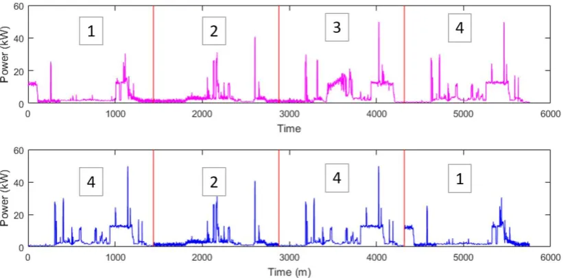
Figure 3.Process of block bootstrap simulation of a new home power usage (bottom) from a template home (top). Example simulation samples are taken from four days from the template series with replacement.

datasets can help model an attacker compromising individual appliances. For each home, the power consumption is given in kW for every minute. We convert this time series to kWh with a resolution of

one hour, which is typical for smart meter readings and RTP modeling [3]. We do this by obtaining the

average power consumption within an hour and multiplying it by the time period as such

E_(kWh)=t_(hr)× 1

60

60

∑

P₍i_kW) (1)

3.2. Block Bootstrap Simulation

In the generation of new time series from sample data, several approaches can be applied depending on the series’ statistical properties. Data that is stationary can be modeled and generated

using an ARMA process [25]. An ARMA model is fitted to the data, and then future data is sampled

from the ARMA distribution. If there is no serial correlation, then the distribution of some sample

data can be modeled using Markov Chain Monte Carlo [26], and new data can be sampled from this

estimated distribution. However, in the case that data exhibited autocorrelation and non-stationarity in the presence of a periodic seasonal pattern, a natural choice is to use the block bootstrap method [27].

The bootstrap method comes from simulation statistics for estimating the distribution of a statistic such as the mean or variance. Bootstrap is particularly useful when there is no analytical form to estimate some underlying distribution. A bootstrap analysis is conducted by using the Monte Carlo algorithms with replacement. Data is sampled with replacement until a new set is formed, and then statistics are calculated from that new set. The process can be repeated to get a more precise estimate of the Bootstrap distribution and form confidence intervals for those statistics. The block bootstrap is used when the data, or the errors in a model, are correlated. The block bootstrap attempts to replicate the serial correlation by resampling blocks of data instead of individual observations. This is why the block bootstrap is used primarily with correlated time series. In block bootstrap, blocks sampled can overlap or be non-overlapping. For load time series simulation, we use block bootstrap with non-overlapping blocks to preserve the daily seasonal pattern of power consumption. The process of

0 10 20 30 40 50 60 70 80 90 100 Price (USD/MWh)

0 1000 2000 3000 4000 5000 6000 7000 8000 9000 10000

Load Demand (MWh)

d = -2 d = -1

d = -0.6 d = -0.4

d = -0.2 d = -0.1

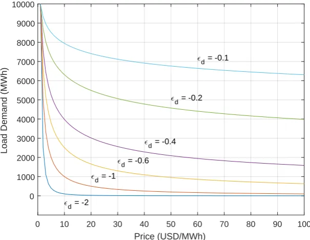
Figure 4. Load as a function of price with arbitrary price range $1-100, α = 10, 000, and ed =

-0.1,-0.2,-0.4,-0.6,-1, -2.

4. Dependency Model

4.1. Modeling Elastic Demand

For analyzing the feedback dependency between load and price in a DSM setting, we first need to define the supply and demand relationship of electricity. To do so we utilize the well-known measure

in economics, the Price Elasticity of Demand (PED) [28] which can be given by

ed= dL dP ·

P

L. (2)

PED shows the responsiveness of the loadLdemanded of electricity to a change in Price (P). Recent

work [9] in demand response, particularly in the context of cybersecurity, has utilized this approach.

Our procedure differs in that we use real demand data to determine the "unmodulated" pattern of

load data. An absolute value of PED = 1 shows unitary elasticity. For instance, whened=−1, then a

1% change in the price will have a 1% change in the load demanded. As prices increase, the load will decrease. When absolute PED falls between 0 and 1, this signifies that the load demand is inelastic,

while a value greater then 1 says that the demand is elastic. When|ed|=0 the demand is perfectly

inelastic. A change in price does not affect the load. Whileed=∞represents perfect elasticity. Ifedis

constant the whole demand curve then,

L=a·Ped ₍₃₎

whereais a scaling constant. An example demand curve estimated from Eq.3can be seen in Fig.4.

The figure also showcases the nonlinear relationship between load and price where as the price, the independent variable, increases the load demanded, the dependent variable, decreases.

4.2. Modeling Consumer DSM

actions such as watching TV or using the AC. Demand is impacted by multiple factors such as user preferences, weather, and time of day. In this process, electricity prices have a small influence on

demand; individual customer demand is fairly inelastic to price. Following the derivation in Eq.3we

define the load usage of an individual customerifor timetas

φt,i =θt,i(Pt+Pc)e

d t,i_,

wherePtis the RTP for timet,Pcis constant of the retailer’s market costs which does not vary with

RTP,θt,i ≥0 is a scaling factor representing the stochastic process that determines the user load, and

ed_t,iis the elasticity coefficient for the individual customers sensitivity to price changes. It can vary over

time but without DSM incentives most users have a fairly inelastic PED.

For experimental purposes, in modeling individual user loads we setφt,i equal to simulated

bootstrapped user load profiles defined in Section3.2. We assume that prices, user preferencesθt,i, and

ed_t,ihave been absorbed in the calculation of the simulated load series. Thus we useφt,ias a reference

point to show how much electricity a user wants to consume without the influence of a DSM program.

We model the task of the demand response administrator as modifyingφt,ito some desired load levels.

Realistically, only a certain portionκt,i ∈[0, 1)of customeri’s power usage will be under control

of a cyber DSM program. There will always be some stochastic and, more importantly, an inelastic component of power usages, such as using a microwave oven or electric hairdryer. We model the DSM modulated load (including the inelastic portion) as follows

lt,i = (κt,iφt,i)P

edsm_t,i

t + (1−κt,i)φt,i, (4)

where the first part(κt,iφt,i)P

edsm_t,i

t is the load level customeriallows the DSM program to determine

as a function of pricePtand the DSM’s elasticity to priceedsm_t,i . Price elasticity of DSMedsm_t,i may vary

over time and customer and affects how much power usage should be affected by price. The second

portion(1−κt,i)φt,i of a customers load is the stochastic component. The DSM portion parameter

κt,iis defined as a function of time where users can add or remove house loads under DSM control

over time. The termκt,ican be modeled as a random variable (e.g. Uniform or Gaussian) or as a fixed

constant for users. Once each customer’s load is determined, total load (modified by a cyber-DSM

program) for timetforNcustomers is calculated by

Lt= N

∑

lt,i. (5)

We also define the aggregate base load as

Φt =

N

∑

φt,i, (6)

which represents the total demand had there not been a DSM program for a time periodt(IEκt,i=0,∀i).

4.3. Modeling Strategic Load Conservation

We propose the following approach to model the real-time pricing from a strategic load conservation perspective, wherein on an hourly basis, the price is a function of the aggregate load to

achieve the desired load levelL0_t. The approach takes as input a forecast ˆΦtof the base aggregate load

to calculate pricePt. This prediction can be defined as

ˆ

Φt= fpred(Φt−k:t−1,Pt−k:t−1,X), (7)

where inputs to the prediction model are past base loadΦand pricePvalues from timet−kto

prediction models can be used for fpredsuch as neural networks as reviewed in section2.2. We now

define RTP based on the formulation in Eq.3as such

Pt=

L∗

ˆ

Φt

1/ ˆedsm

L∗=a·Peˆdsm

t

. (8)

Where, we can have two goal scenarios forL∗

Goal 1:L∗=L0_t

Goal 2:L∗=L0t+ (Lt0−1−Lt−1)

. (9)

The componentL∗adjusts the RTP based on two goals the ISO may have. The first goal is to adjust

the price to push power usage directly to the target levelL0_twith the assumption that there is near

100% DSM participation by all customers. The expectation is that if demand for timetis ˆΦt, then a

price point is set to push load usage toL0_t. Of course, if participation is less then 100%, which is more

likely, the target levelL0_twill not be reached byPt. To push the aggregate load from all users, as close

as possible to the target load level with an unknown amount of participation, a penalty would need to

be added toPt. We model this as Goal 2, where the idea is to affect the power usage of those under

cyber-DSM control even more than goal 1 to compensate users who are not participating in DSM. Some users will not be participating, or only have a small portion of their power usage under control by the cyber-DSM program. We model their remaining power usage as inelastic to RTP. Thus, to push aggregate load to a target level, taking into account some load usage is inelastic, we need to push RTP much higher or lower to have a bigger effect in pushing DSM controlled load closer to the

target load. This is what Goal 2 attempts to do, with the componentL∗=L0t+ (Lt0−1−Lt−1)taking the

target load level for timetand adding the difference from the previous target loadL0_t−1and realized

loadLt−1as a penalty to adjust RTP to compensate for the difference. IfL∗<0 then we setL∗=10

or to some arbitrary small target value. By subtracting the difference between the previous load and target level, we make up for users not participating in DSM by forcing DSM users a higher price to push their load even lower.

The term ˆedsmin Eq.8is an estimate of the price elasticity of DSM of the whole grid; if individual

user coefficientsedsm_t,i are unknown then ˆedsmcan be estimated from observing past values of price and

load under different levels of DSM control. Alternatively, the ISO can defineedsmfor all household

cyber DSM programs. The formulation in Eq.8sets prices by comparing the adjusted target load for

timetto the forecasted base demand ˆΦtfor the same time. This demand ˆΦtwould be the level if no

load were under DSM influence, thus to influence and alter it,Φtneeds to be estimated as accurately

as possible.

In our approach, if the aggregate load is above the target load, RTP is set higher to decrease demand. If the aggregate load is lower than the target load, the price decreases to increase demand.

Thus, as also can be observed in Eq.8, there is direct feedback between price and load Eq.4. The block

diagram in Fig.5also outlines this feedback that showcases the relationship between the utility and

the grid. Generation sets the target load based on the price and supply of power, and the controller sets the price signal and the elasticity of demand coefficient for DSM systems. The price is then communicated into the grid into DSM systems, which adjust load usage appropriately. The bold red

lines in Fig.5highlight the feedback relationship between price and demand. The scope of work is in

X

𝜖

𝑃

𝐿

𝜑

DSM System

X

𝐿

𝜑

𝐿

Controller

𝜖

𝑃

External Factors

𝐿

𝑃

Generation

Smart Grid

Utility

Figure 5.Block diagram highlighting the feedback between the utility and grid.

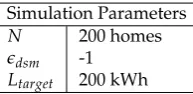
Simulation Parameters

N 200 homes

edsm -1

Ltarget 200 kWh

Table 1.Simulation parameters used in case studies.

4.4. Simulation Parameters and Assumptions

For experimental purposes, in modeling individual user loads we setφt,i equal to simulated

bootstrapped user load profiles defined in Section3.2. We assume that prices, user preferencesθt,i, and

ed_t,ihave been absorbed in the calculation of the simulated load series. Thus we useφt,ias a reference

point to how much electricity a user wants to consume without the influence of a DSM program. We

model the task of the ISO as modifyingφt,ito some desired load levels. Furthermore, we include the

following assumptions in our modeling and simulation. We assume the ISO can defineedsmfor each

household and we set it as a constant for all customers and time. For additional simplicity, we model

κialso invariant in time, but it may vary per customer. Lastly, through AMI, we assume the ISO can

obtain an estimated reading ofΦt−1but not of individual userφt−1,ito preserve privacy. This way the

ISO has a time series of estimated non-DSM load demand in order to provide predictions ˆΦt.

For all case studies in the rest of our paper, we use the UMass Smart* dataset (2017 release) to

bootstrap simulate residential load as described in Section3. We simulate a micro-grid ofN=200

residential homes for a time period ofTto obtain aphidistribution that defines a base load profile for

each homeiat each timet. We set the DSM demand elasticity for each user toedsm=−1,∀ito allow

the DSM component of customer load to be sensitive enough to price changes. For all case studies we

set a simple flat target load ofLtarget=200 kWh. We note, however, that with our pricing formulation

in Eq. 8, we can model any DSM goal from peak load reduction to flexible load shaping. These

simulation parameters are summarized in Table1. For forecasting ˆΦtwe use the naive persistence

prediction method.

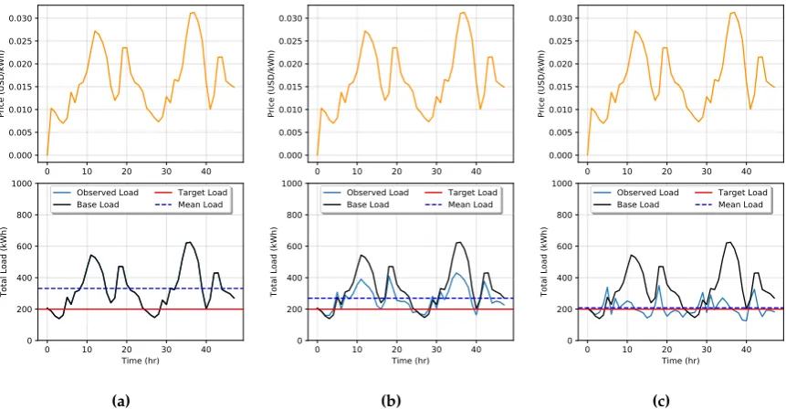
In Figures6and7we demonstrate a price-load feedback simulation for a period ofT=48 hrs

under Goals 1 and 2 with parameters defined in Table1. Under the Goal 1 scenario whenκi =0,∀i,

shown in Fig.6(a), we see that prices range from $0.01 to $0.03 per kWh. As expected with no DSM

0 10 20 30 40 0.000 0.005 0.010 0.015 0.020 0.025 0.030 Price (USD/kWh)

0 10 20 30 40 Time (hr) 0 200 400 600 800 1000

Total Load (kWh)

Observed Load

Base Load Target LoadMean Load

(a)

0 10 20 30 40 0.000 0.005 0.010 0.015 0.020 0.025 0.030 Price (USD/kWh)

0 10 20 30 40 Time (hr) 0 200 400 600 800 1000

Total Load (kWh)

Observed Load

Base Load Target LoadMean Load

(b)

0 10 20 30 40 0.000 0.005 0.010 0.015 0.020 0.025 0.030 Price (USD/kWh)

0 10 20 30 40 Time (hr) 0 200 400 600 800 1000

Total Load (kWh)

Observed Load

Base Load Target LoadMean Load

(c)

Figure 6.Simulation of price-load interaction with Goal 1 with DSM whenκi=0,∀i(a),κi=0.5,∀i

(b), andκi=0.99,∀iin (c).

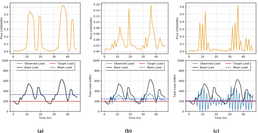
7(a) when the simulation is run with the Goal 2 RTP model. The only difference under this scenario is

the price range which is exceptionally high ranging from $0.01 to $0.6 per kWh. This is expected in this scenario since the ISO is attempting to set prices to maximize the effect on DSM customers, which there are none, but this is unknown to the utility. With no DSM the mean observed load is 332 kWh.

Next, we rerun the simulation settingκi =0.5,∀i. In the Goal 1 scenario in Fig.6(b) we see that

the base load was reduced with a mean observed load of 269 kWh. In Fig.7(b) the same simulation

is run with Goal 2. Here the mean observed load was further reduced to 246 kWh, but large price

spikes occur at peak load times. Finally, we run simulations forκi =0.99,∀i to study the effects of

high penetration of DSM. In simulating both goals, shown in Figures6(c) and7(c), the mean observed

load is reduced to 208 kWh, which is very close to the target load. However, in Goal 2, we see great resonating feedback effects occur when prices spike very high. RTP increases as a response to large values in the observed load. Then when the load decreases to low levels, prices decrease cause load to spike more during the next time step. While under Goal 1, this is not observed. The higher prices set in Goal 2 would see a large cost to DSM participating customers.

5. DSM Attack Models

An attacker can exploit the feedback between the customer and utility in determining RTP and load usage by cyber DSM programs by injecting false price or corrupted load data into the feedback loop. The attack exploitations we study here differ from the false data injection attacks studied in

other smart grid papers. Most false data injection attack works [29] study the compromise in energy

management systems to alter power state estimates by the utility operator. In our case, we study attacks that aim to alter a user’s load profile by exploiting cyber DSM vulnerabilities.

For modeling attacks on a cyber DSM managed micro-grid, we assume that the attacker

compromises a subset of all the N customers; we denote this subset as A, for an attack period

t∈Ta. We study two modes of attacks: false pricing data injection attacks in which a compromised

0 10 20 30 40 0.0 0.1 0.2 0.3 0.4 0.5 0.6 Price (USD/kWh)

0 10 20 30 40 Time (hr) 0 200 400 600 800 1000

Total Load (kWh)

Observed Load

Base Load Target LoadMean Load

(a)

0 10 20 30 40 0.00 0.02 0.04 0.06 0.08 0.10 0.12 0.14 0.16 Price (USD/kWh)

0 10 20 30 40 Time (hr) 0 200 400 600 800 1000

Total Load (kWh)

Observed Load

Base Load Target LoadMean Load

(b)

0 10 20 30 40 0.0 0.1 0.2 0.3 0.4 0.5 0.6 Price (USD/kWh)

0 10 20 30 40 Time (hr) 0 200 400 600 800 1000

Total Load (kWh)

Observed Load

Base Load Target LoadMean Load

(c)

Figure 7.Simulation of price-load interaction with Goal 2 with DSM whenκi=0,∀i(a),κi=0.5,∀i

(b), andκi=0.99,∀iin (c).

• False Pricing Data Injection: The attacker can manipulate prices Pt received by each

compromised costumeri∈ A, and the received priceP_tican be different for various customers in

order to achieve the attacker’s desired effect:

P_ta_,i=Pt,i+aPt,i,∀i ∈ A,t∈Ta

This has the affect of compromising the demand response of a customer in the following way:

l_ta_,P_i = (κiφt,i)(atP,i)e

dsm

+ (1−κi)φt,i

• Direct Load Manipulation: The attacker can manipulate the load of each compromised customer

lt,i,i∈Ddirectly:

l_ta_,L_i =lt,i+aLt,i,∀i ∈ A,t∈Ta

Under both attack modes, we would get a compromised aggregate load which may include one or both attacks occurring simultaneously

Lat = N

∑

la_t,P_i +l_ta_,L_i.

These two modes of attack are equivalent as they both affect a customers load response as long a part of the load is under cyber DSM control that is sensitive to price changes.

Theorem 1.Given a set of customersAcompromised by the attacker, there always exist a direct load manipulation attack such that all customers behave the same as a pricing data injection attack and vice

versa forκi>0,∀i,t∈Ta.

Proof. Setting both attacks to have the same load, then the attack load is set as follows

aL_t,i= (κiφt,i)(aPt,i)e

dsm

0 10 20 30 40 0 50 100 150 200 250 Attack Level

0 10 20 30 40 Time (hr) 0 200 400 600 800 1000

Total Load (kWh)

Attacked Load Nominal Load

(a)

0 10 20 30 40 0 25 50 75 100 125 150 175 200 Attack Level

0 10 20 30 40 Time (hr) 0 200 400 600 800 1000

Total Load (kWh)

Attacked Load Nominal Load

(b)

0 10 20 30 40 0 50 100 150 200 250 300 Attack Level

0 10 20 30 40 Time (hr) 0 200 400 600 800 1000

Total Load (kWh)

Attacked Load Nominal Load

(c)

Figure 8.Examples of different type of DSM attacks: (a) ramp attack, (b) sudden attack, and (c) point attack.

and the equivalent attacked price is

aP_t,i= a L

t,i−(1−κi)φt,i

κiφt,i

!1/edsm

Ifκi = 0 then the two attack modes are not equivalent since a price attack will have no affect on

customer load.

Since false pricing data injection and direct load manipulation attacks are equivalent, we focus only on direct load manipulation attack analysis.

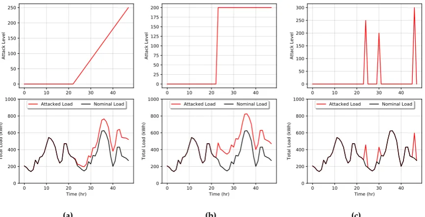
There are different goals an attacker can have to harm the power grid or exploit it. For example, an attacker can cause chaotic metering by messing the metering data transmission, efficiency loss of the energy provided by causing higher load volatility, or the energy system failure by overloading the power lines or devices. The focus of this work is efficiency loss by increasing user loads through direct load manipulation. In this scenario, we introduce three possible types of load attacks: ramp,

sudden, and point attacks. These types of attacks are visualized in Fig.8wherein plot (a) an attacker

gradually increases a user’s load over time. In plot (b) an attacker suddenly ramps up the power usage to a specified level, and in plot (c) we demonstrate a point attack where the attacker increases loads only for specific hours.

6. Attack Detection

Here we outline sequential parametric, supervised learning-based, and nonparametric methods for attack detection. The sequential detections methods are the one-sided CUmulative SUM (CUSUM)

test [30] and windowed GLRT [31]. Both these methods take as an input a residual time series that is

the output of applying a SARIMA filter to load observations. If enough past observations of load data labeled as nominal or under attack are collected, then detection of attacks can be made by training supervised learning classifiers. Supervised learning algorithms have been broadly adopted to the

smart grid literature to monitor and detect cyber attacks on power systems [32–34]. Here we employ

data can be simulated. Using past load data, we simulate direct load manipulation attacks by creating

different types of attacks, as shown in Fig.8.

6.0.1. SARIMA Model

In almost all our detection models, a Seasonal AutoRegressive Integrated Moving Average (SARIMA) forecast of load demand is used. Mathematically, the SARIMA model is denoted as

SARI MA(p,d,q)(P,D,Q)(S), whereSrefers to the number of time units in each season,pandqare

the autoregressive and moving average terms for nonseasonal part,dis the degree of differencing (the

number of times the data have had past values subtracted) and the uppercaseP,DandQrefer to the

autoregressive, differencing and moving average terms for the seasonal part of the ARIMA model. We can write the model as the following equation

(1−

p

∑

αiB)(1− P

∑

βiBS)(1−B)d(1−BS)DY(t+1)

= (1+ q

∑

uiB)(1+ Q

∑

γiBS)x(t+1)

whereBis the back-shift operator of the model,αi,βi,ui, andγiare fixed coefficients determined

by the model after capturing the behavior of the series.Y(t+1)is the price or load data at timet+1

andx(t+1)is the residual of the data. The exponents in the equation represent the times that the

back-shift operator is multiplied.

6.1. Sequential Detection Methods

In sequential change-point detection, a series does not have a fixed length. Instead, observations are received and processed sequentially over time. When an observation is received, a decision is made about whether a change has occurred in the state. This is based only on the observations that have been received so far or within a fixed past window size. If no change is detected, then the next observation in the sequence is processed. The sequential formulation allows sequences containing multiple change points to be easily handled. Sequential change-point detection can be applied in the case of attack detection to identify if a load time series has been compromised. If an attack is flagged, an ISO can take appropriate actions to prevent further damage to the grid.

In the parametric detection realm, the Generalized Likelihood Ratio Test (GLRT) is a popular and influential method; it has been widely used in anomaly detection and signal detection. The advantage of the GLRT is that it can provide estimates of the unknown shift in statistical parameters and has

consequently been used to distinguish different types of anomalies [35]. However, its applicability relies

on knowledge of the statistical parameters when a system is not under attack, and the effectiveness

reduces with an increasing number of unknown parameters. In [36], H.B. Mann and D.R. Whitney

first presented the theory of creating a new statistic for a sequence of data to detect a probabilistic

change without knowing any distribution information of the data. In [37], Ming Yu illustrated several

features for nonparametric detection in network anomaly detection: (1) no assumption is made on the distribution of observations. (2) its detection threshold is self-adjusted, and (3) it can react to the

end of an anomaly within a required delay time. In [38], Hawkins employed an idea of dividing

data into windows to analyze data anomaly in a window with the adjustable window size using a nonparametric method. In this work, we adapted Hawkins’s idea and designed a moving window nonparametric detector to detect false data injection attacks in real-time.

Under the Sequential Detection paradigm, we collect observations and apply a whitening filter to produce a continuing series with the assumption that it is white Gaussian noise. If an additive

attackAt >0 is present for observationt, this will cause a definite shift in the mean of the residual

residual series has zero mean and known variance (invariant in time and estimated from a sample

population), or if the alternative hypothesisH₁is correct which states that the examined series has

some mean not equal to zero thus being under attack. This can be modeled as a hypothesis test, and for the GLRT and CUSUM detectors this translates to

H0:xt∼ N(0,σ2),t=1, ...,N

H₁:xt∼ N(At,σ2),At>0,t=1, ...,N

For the GLRT detector, to simplify implementation, we model the attack as if it were constantA>0

but unknown. To produce a residual series, a SARIMA multi-step forecast fort= 1, ...,Nis made

before the detection period. This forecast is conducted using a past window of training data that was

not under attack. The forecast is made for timettot+k. These predictions are then subtracted from

the incoming observations to produce a residual time series, which is then fed as input into the GLRT and CUSUM detectors.

6.2. Nonparametric Detection Methods

We look at two nonparametric detectors: CUSUM and Mann–Whitney. CUSUM is a classic nonparametric detection method. A CUSUM test is a control chart that is used to monitor the mean of a process based on samples taken from past data at specific time intervals. It is a class of non-linear stopping rules for structural changes. Given information on current and previous samples, a CUSUM

test relies on the specification of a target valuehand a known or reliable estimate of the standard

deviationσthe process. The CUSUM test typically signals an out of control or anomalous process by

an upward or downward drift of the cumulative sum until it crosses the target threshold. If the mean of the load series shifts above the target threshold for attack detection, we assume the grid is under attack.

We define the CUSUM detector as follows. Taking the residual seriesxt =yt−Et−1[yt], again

defined by a SARIMA forecastEt−1[yt], we define a one-sided CUSUM detector as

gt=max(0,gt−1+xt−k)

wherekis called the reference value (sometimes also called drift) set priori to values such as 0, 0.5,

orA/2 if the size ofAis known in advance. Whengt=0 then we define the change time astc=t,

and whengt>h>0 we resetgt=0 and flag an alarm at timeta=T. The alarm threshold is also set

priori to some value based on the sample population standard deviation such ash =2σwhereσis

estimated from past training data used to produce the SARIMA forecasts.

Building off the CUSUM, a more sophisticated nonparametric detector is the Mann–Whitney

method. Following the approach in [36], we consider a sequence of data samples sorted into descending

order. Each of them haskelements from setXandn−kelements from setY. We label elements from

Yasa1,Xasa0. LetPk,n−k(U)represent the probability of a sequence in whicha1precedesa0Utimes.

We define the following statistic from the data

Uk,n−k= n

∑

k

∑

ψ(Xi−Xj)

whereψ(t)is the unit step function (ψ(t) =0,t<0 andψ(t) =1,t≥0). Consequently, we can write

Pk,n−k(U) = k

nPk−1,n−k(U−n+k) + n−k

Following the approach in [36], we get

Ek,n−k(U) =

k(n−k)

2

Vark,n−k(U) =

k(n−k)(n+1)

12

Placing thendata points into a window and utilizingkas a moving split point, the pre split sequence

isa0and the post-split sequence isa1.

When the data is under attack, by computingUk,n−kfor different values ofk, the detector can

determine a suspect start point of the attack. The algorithm can be illustrated by the following equation

Tmax,k,n−k= max 1≤k≤n−1{

|Uk,n−k−k(n

−k) 2 | q

k(n−k)(n+1) 12

}

¯

T_T=arg max

1≤k≤n−1(Tmax,k,n−k)

where Tk,n−k is the test statistic of the detector, Tmax,k,n−k is the maximum value of the Tk,n−k by

traversingkin 1≤k≤n−1 and ¯TTis the correspondingkwhen theTmax,k,n−kis located. With all

previous discussion, we can introduce a specified control limithnand create a hypothesis test

• ComputeTmax,k,n−k, the maximized split statistic.

• IfTmax,k,n−k ≤hn, then conclude that the data in this window is in control without attack and

continue to move the window forward along the whole sequence of data.

• IfTmax,k,n−k>hn, then conclude that the data in this window is under attack and stop the process

of moving the window for diagnosis. Estimate the epoch of attack start point by the maximizing

k, which is ¯TT.

6.3. Supervised Learning Methods

Changepoint detection could alternatively be seen as a supervised learning binary classification problem. Under this scheme, all of the change point sequences, or in our case attacks, represent one class, and all of the nominal sequences represent a second class. Supervised learning methods are machine learning algorithms that learn a mapping from input data to a target class label. Given a

set of samplesX = {xi}Ni=1and a set of labelsY ={yi}iN=1, then the supervised learning detection

problem is defined as a hypothesis function that captures the relationship between samples and labels

f :X −→ Y. A sliding window moves through the data, considering each difference between two data points as a possible change point.

An advantage of treating attack detection as a supervised learning problem is that it has a more straightforward training phase. However, a sufficient amount and diversity of training data need to be provided to represent all of the classes of attacks. To ensure enough training data, and to prevent class label imbalance, we simulate all attack data to train our algorithms. Machine learning methods

have successfully been applied several times in data injection attacks in power systems [33,34], so

we analyze here their ability to detect data attacks on cyber-DSM systems. The binary classification problem for attack detection can be defined as

yi =

(

1, ifAi >0

0, ifAi =0

whereyi = 1 if thei-th observation is under attack, andyi = 0 if there is no attack. A variety of

time axis

time axis

prediction _{past data}

past data

nominal attack

attack

nominal nominal

TN FN TP FP

true

detection window

Figure 9.Confusion matrix imposed on a time axis of attack predictions vs true observations.

compelling and have widespread use in both industry and academia; model descriptions of these

methods can be found in [39,40]. All these models were implemented using the Python package

scikit-learn [41] with each model using default parameters from the package.

6.4. Performance Analysis

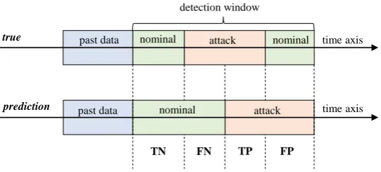
For the security of cyber DSM systems, the major concern is not just the detection of attacks, but also the detection of nominal data with high reliability. We want a detection system that can predict not only with high accuracy but also with high precision and recall to avoid false alarms. Therefore, we measure the True Positives (TP), the True Negatives (TN), the False Positives (FP), and the False

Negatives (FN). Definitions of these measures are visually shown in Fig.9. We use these measures to

calculate several main performance indicators of accuracy, precision, and recall.

We calculate accuracy as the ratio of correctly classified data points to total data points

Accuracy= TP+TN TP+TN+FP+FN

This measure provides the total classification success of the models. But alone, accuracy is not enough to get a full picture of performance. Precision is calculated as the ratio of true positive data points (attacks) to total points classified as attacks

Precision= TP TP+FP

On the other hand, recall, also known as the True Positive Rate (TPR), refers to the portion of attacks that were recognized correctly

Recall = TP TP+FN

Precision values give information about the prediction performance of the algorithms, whereas recall values measure the degree of attack retrieval. For instance, a recall value equal to 1 signifies that none of the attacked measurements were misclassified as nominal.

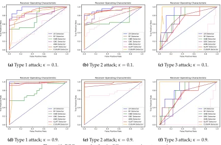
We use one more final measure of total performance of our detectors, the Receiver Operating Characteristics (ROC) curve. The ROC curve is an assessment that enables visual analysis of the trade-off between TPR and False Positive Rate (FPR). This can also be seen as the trade-off between the probability of detection and the probability of false alarm. FPR is defined as follows

FPR= FP

FP+TN.

0.0 0.2 0.4 0.6 0.8 1.0 False Positive Rate

0.0 0.2 0.4 0.6 0.8 1.0

True Positive Rate

Receiver Operating Characteristic

LR Detector RF Detector GNB Detector GBC Detector ANN Detector GLRT Detector CUSUM Detector

(a)Type 1 attack;κ=0.1.

0.0 0.2 0.4 0.6 0.8 1.0 False Positive Rate

0.0 0.2 0.4 0.6 0.8 1.0

True Positive Rate

Receiver Operating Characteristic

LR Detector RF Detector GNB Detector GBC Detector ANN Detector GLRT Detector CUSUM Detector

(b)Type 2 attack;κ=0.1.

0.0 0.2 0.4 0.6 0.8 1.0 False Positive Rate

0.0 0.2 0.4 0.6 0.8 1.0

True Positive Rate

Receiver Operating Characteristic

LR Detector RF Detector GNB Detector GBC Detector ANN Detector GLRT Detector CUSUM Detector

(c)Type 3 attack;κ=0.1.

0.0 0.2 0.4 0.6 0.8 1.0 False Positive Rate

0.0 0.2 0.4 0.6 0.8 1.0

True Positive Rate

Receiver Operating Characteristic

LR Detector RF Detector GNB Detector GBC Detector ANN Detector GLRT Detector CUSUM Detector

(d)Type 1 attack;κ=0.9.

0.0 0.2 0.4 0.6 0.8 1.0 False Positive Rate

0.0 0.2 0.4 0.6 0.8 1.0

True Positive Rate

Receiver Operating Characteristic

LR Detector RF Detector GNB Detector GBC Detector ANN Detector GLRT Detector CUSUM Detector

(e)Type 2 attack;κ=0.9.

0.0 0.2 0.4 0.6 0.8 1.0 False Positive Rate

0.0 0.2 0.4 0.6 0.8 1.0

True Positive Rate

Receiver Operating Characteristic

LR Detector RF Detector GNB Detector GBC Detector ANN Detector GLRT Detector CUSUM Detector

(f)Type 3 attack;κ=0.9. Figure 10.ROC curves for the six different experiment scenarios.

close to the upper axes boundary is reflective of a good detector. The best possible detection method would produce a point in the upper left corner, coordinate (0,1) of the ROC space. A random prediction would give a point along a diagonal line from (0,0) to (1,1). Points above this line are considered to have performance, while points below are considered with performance worse than guessing.

7. Detection Experiments and Results

For attack simulation and detection experiments, we use all the same parameters from Table1, but

we varied the levels ofκand attacksat. We simulate each of the three types of attacks, as visualized in

Fig.8, each in the form of direct load manipulation attack, under DSM participation levelsκ=0.1 and

0.9. This creates a total of six experiment scenarios. For each scenario, we simulate 28 days of training data (672 observations) and two proceeding days of test data (48 observations), both at a resolution of 1 hr. All training data is created nominally with no attacks. In the test data sets, the first 24 hrs of the test data are not under attack. In the last 24 hours of the test data, we add one of the three types of attacks.

For ramp attacks, for each time step we add an attackat=at−1+5 where the first 24 hours of the test

setat=0...23=0. The sudden attacks are similar except the attack is an additive constantat=150. The

last type of attack, point attacks, areat=24 =250,at=29 =200,at=34 =300,at=37 =100,at=46 =150,

andat=0 everywhere else. To showcase a wide variety of detection strategies, we conduct two main

Table 2.Evaluation metrics for attack detection.

κ 0.1 0.9

Attack Type 1 2 3 1 2 3

Accuracy

LR 89.6 100.0 87.5 87.5 100.0 75.0

RF 77.1 97.9 64.6 77.1 93.8 60.4

GNB 70.8 77.1 75.0 79.2 100.0 72.9

GBC 85.4 97.9 66.7 85.4 100.0 64.6

ANN 56.3 95.8 20.8 75.0 79.2 14.6

GLRT 79.2 95.8 58.3 91.7 97.9 58.3

CUSUM 83.3 95.8 95.8 87.5 100.0 100.0

Recall

LR 92.0 100.0 80.0 89.0 100.0 80.0

RF 56.0 96.0 80.0 56.0 88.0 80.0

GNB 88.0 56.0 80.0 60.0 100.0 80.0

GBC 76.0 96.0 100.0 88.0 100.0 80.0

ANN 68.0 92.0 60.0 76.0 68.0 80.0

GLRT 76.0 92.0 80.0 84.0 96.0 80.0

CUSUM 80.0 96.0 100.0 84.0 100.0 100.0

Pr

ecision

LR 88.5 100.0 44.4 88.0 100.0 26.7

RF 100.0 100.0 20.0 100.0 100.0 18.2

GNB 66.7 100.0 26.7 100.0 100.0 25.0

GBC 95.0 100.0 23.8 84.0 100.0 20.0

ANN 56.7 100.0 7.7 76.0 89.5 9.1

GLRT 82.6 100.0 17.4 100.0 100.0 17.4

CUSUM 87.0 96.0 71.4 91.3 100.0 100.0

7.1. Sequential vs Supervised Learning Detection

For the sequential detectors, we use multi-step SARIMA forecasts to predict the next 48 hrs and then use those forecasts to filter incoming test data for detection. The training was conducted on the training time series of 28 days of nominal data. SARIMA hyperparameters were chosen by examining lag one differenced AutoCorrelation Function (ACF) and Partial AutoCorrelation Function (PACF) plots of the training data. These forecasts where then subtracted from the incoming test data to obtain a residual series that is input to the sequential detectors. The assumption for both detectors is that the residual series is Gaussian white noise, where the series has zero mean, and each observation is independent identically distributed from a Gaussian distribution.

0 10 20 30 40 50 0.25

0.00 0.25 0.50 0.75

1.00 Autocorrelation

0 10 20 30 40 50 0.0

0.5

1.0 Partial Autocorrelation

80 60 40 20 0 20 40 60 80 Theoretical quantiles

100 50 0 50 100 150

Ordered Values

Q-Q Plot of Training Residuals

Figure 12.Q-Q plot of the residual series between the SARIMA fit tp training data. From the plot we observe that for extreme quantiles the distribution is not Gaussian.

To ensure the residuals are white noise we apply the Augmented Dickey-Fuller (ADF) test to check for stationarity, we examine the ACF/PACF plots to check for independence and run a Jarque-Bera test, and we examine a Q-Q plot to check if the residual series has a Gaussian probability distribution. We conduct these checks on all scenario training datasets, where we first train a SARIMA fit on them and then subtract that fit to produce the residual series. In all the training data sets, the residuals were stationary from the ADF test and independent from ACF/PACF plots. However, the Jarque-Bera test and Q-Q plots showed that the observations did not come from a Gaussian distribution. Example,

ACF/PACF and Q-Q plots forκ=0.1 are shown in Fig.11and Fig.12. Despite the residuals not being

Gaussian, we still run the sequential detectors and examine their performance.

For training the supervised learning methods for each of the six scenarios, we simulate more data to ensure proper class learning. We keep the test sets the same, but we extend each training set doubling its size. We keep the original training set, labeling it as nominal, and then make a copy of it. In the copy, we split it into three parts, each part we add one of the types of attacks at random levels. We label each observation of this set as under attack. We added the nominal and attacked training sets to form a new training set with a total of 1,344 observations. With our training and test time series,

we then create a setX features andY labels that could be fed into the supervised learning classifiers.

Each training samplexi∈ X is composed of 24 hours of lagged data, each hour is one feature, and

each labelyi∈ Y corresponds to a class 0 (not under attack) and class 1 (under attack). Together we

getN=1, 298 pairs of(xi,yi)training samples.

We run our experiments on a computer with an Intel i7 6700 2.6 GHz and 16 GB of RAM. Implementation of the simulations, experiments, and sequential detectors were done in Python

3.6. Implementation for SARIMA forecasts was done using the Python package Statsmodels [42],

the supervised learning methods and confusion evaluation metrics were implemented using the

Scikit-Learn Python package [41], and ROC curves were created using the Matplotlib Python package

[43]. All classifiers used default hyperparameters from Scikit-Learn. We compiled all code and data

used in our work into a Python package titled LehighDSM, which is publicly available on GitHub [44].

Experimental results from the six scenarios are reported in Table2, in the form of accuracy, recall,

and precision metrics, and Fig. 10which showcases six ROC curves, one for each scenario. All

performance measures in Table2, were calculated using the best thresholds found in the ROC curves

by searching for the shortest distance from each curve to the corner (0,1). As seen in Fig.10(c,f) type 3

attacks, under any DSM level, had the lowest detection rates across thresholds with ANN being the

worst performer. In Fig.10(a,d) LR yielded the best performance with GNB, and again ANN being the

worst. Type 2 attacks in Fig.10(b,e) resulted in the best detection with CUSUM, LR, GNB and GBC

Figure 13.Performance comparison between parametric and nonparametric detector under 200 number of users.

With the results from Table2, we have the following conclusions; demonstrated findings imply

that detection of attacks has a higher accuracy with higher levels of DSM participation. This occurs since higher DSM penetration results in more aggregated attacks. However, we note that an attacker, if having perfect knowledge of the grid, could decrease their intensity and make detection more difficult. Furthermore, the supervised learning classifiers’ performance on average was on par or better than sequential detection methods. From a detector comparison perspective, the parametric and nonparametric detectors showcased higher performance on most of the attacks and varying parameters. In the following section, we do a deeper dive on a comparison between the GLRT and the nonparametric detectors to derive further inferences on operations paradigms for the attack detection problem.

7.2. GLRT Detection Versus Nonparametric Detection

For the comparison between the nonparametric detector and parametric GLRT detector, we conduct our numerical experiments using the block bootstrap approach on real demand data (unmodulated by DSM) available from the New England ISO, to generate demand for 7 to 200

users. We apply the price-elasticity model with the DSM participating rate ofkand pricing information

from the New England ISO to generate the DSM modulated price and demand for multiple time periods. We first compare the performance of the GLR and nonparametric detectors on identical data

windows in Figures 13 and 14.Pdenotes the DSM participation rate,kmeans the percentage of the

Figure 14.Performance comparison between parametric and nonparametric detectors with two users only.

There are a few key observations from Figures13and14. First, as expected, the performance

of both detectors improve with attack magnitude. Second, the nonparametric detector outperforms the GLRT for small user sizes, whereas the comparison yields the opposite conclusion in the 200 user simulation. The reasoning behind this observation is that: when fewer users’ data is analyzed, the residuals based on the SARIMA forecasts are far less likely to behave like white noise, and consequently, the GLRT optimized for Gaussian residuals underperforms. The nonparametric detector, aside from not requiring the legitimate statistics, purely checks for statistical shifts and performs better in a smaller user pool. In a larger user pool, we enter a law of large numbers regime, where the aggregate residuals increasingly resemble Gaussian variables, and thus the optimized GLRT has a better ROC curve.

Figure 15.Performance comparison between nonparametric and GLRT detector, N = 2,PFA= 0.1, P =

20%, k = 30%.

Fig.15plots the performance comparison as a function of attack magnitude and window sizes for

a fixed false alarm probability (PFA). As expected, the GLRT outperforms the nonparametric detector

when statistical variations are small (due to fewer users, smaller attack magnitude or lower delay), nonparametric detectors are appropriate.

8. Conclusion

In this work, we study the exploitation of the hypothetical feedback between cyber-enabled DSM programs, on the consumer side, and dynamic RTP on the utility side. An attacker with exploitive economic or nefarious intentions, such as causing efficiency loss of energy provision, can take advantage of the dependency between dynamic pricing and DSM load control. The utility modifies prices in response to forecasted demand in order to push realized load up or down. This is done to achieve some target load level to reduce peak load or achieve some other DSM objective. On the user side, cyber DSM programs then autonomously respond to prices to adjust certain portions of a user’s load up or down with some given elasticity.

We propose two modes of attacks, false price data injections, and direct load manipulation. Under a false price data injection, an attacker modifies the RTP that users receive to alter their demand. Through a direct load manipulation attack, attacker hacks and alters a user’s load profile directly. In both these attacks, aggregate load from the grid is modified, which can alter future prices or demand. We showcase how these two modes of attacks are equivalent and introduce three ways an attack can occur. The first type is a ramp attack, the second is a sudden attack, and the third is a point attack. We simulate these types of attacks and review several methods to detect them.

We simulate and examine load-price data under different DSM participation levels with three types of additive random attacks: ramp, sudden, and point attacks. We then conduct two tutorial-style detection studies. First, we compare sequential change point and supervised learning methods. Moreover, in a second study, we compare parametric and nonparametric detectors under different conditions. These two studies are meant to provide a broad review of various possible detection approaches. Results conclude that higher amounts of DSM participation can exacerbate attacks and lead to better detection of such attacks, point attacks are the hardest to detect, and supervised learning methods produce par or better results than sequential detectors. Amongst the GLRT based parametric and the nonparametric detector, we show that with growing window size, the performance of both the detectors will increase. The performance of the GLRT detector increases faster when the detection horizon increases due to the MLE mechanism. So if the detection horizon is broad and the user number is fixed, both the detectors become more potent due to the more information and larger size of the attack data.

Due to the speculative nature of these types of attacks, we plan to look into many different issues for future studies. New directions include expanding our model to incorporate day ahead pricing and DSM scheduling, adding models of cost and utility on for a customer and ISO, expanding our model taking into account grid topology, and modeling advanced attack goals such as system failure by power line overload. Additionally, in this work, we only looked at the DSM goal of strategic load conservation. More complex strategies, such as load shifting, could result in more complex types of cyber attacks; this also makes for compelling future work.

Acknowledgments:This work is supported by the Department of Energy through Award Number DE-OE0000779.

References

1. Faruqui, A.; Sergici, S. Household response to dynamic pricing of electricity-A survey of the empirical evidence. Available at SSRN 11341322010.

2. Grochocki, D.; Huh, J.H.; Berthier, R.; Bobba, R.; Sanders, W.H.; Cárdenas, A.A.; Jetcheva, J.G. AMI threats, intrusion detection requirements and deployment recommendations. 2012 IEEE Third International Conference on Smart Grid Communications (SmartGridComm). Citeseer, 2012, pp. 395–400.