Exponentially stable solution of mathematical model of agents dynamics on time scales

(1)

R E S E A R C H

Open Access

Exponentially stable solution of

mathematical model of agents dynamics on

time scales

Ewa Schmeidel

1*

_{, Urszula Ostaszewska}

1

_{and Małgorzata Zdanowicz}

1

*_{Correspondence:}

[email protected]

1_{Institute of Mathematics, University}

of Bialystok, Białystok, Poland

Abstract

This work is an attempt at studying leader-following model on the arbitrary time scale. The step size is treated as a function of time. Our purpose is establishing conditions ensuring a leader-following consensus for any time scale basing on the Grönwall inequality. We give some examples illustrating the obtained results.

MSC: 34N05; 34D20; 93C10

Keywords: Time scales; Leader-following problem; Grönwall inequality; Multi-agent systems; Graph theory

1 Introduction

The aim of this paper is to propose conditions ensuring the consensus of a multi-agent sys-tem over an arbitrary time scale. We consider continuous- and discrete-time models and also models on time scales simultaneously consisting of both kinds of points, right-dense and right-scattered. Under some assumptions, we prove that consensus can be achieved exponentially if the graininess function is bounded. All theorems are still true if the grain-iness function approaches zero. Some existing results of discrete-time consensus are par-ticular cases of the results presented in this paper.

The leader-following problem has been investigated since 1970s. In 1974, DeGroot [1] studied an explicitly described model that resulted in the consensus. In 2000, Krause [2,

3] discussed the model of a group of agents who have to make a joint assessment of a certain magnitude. The coordination of groups of mobile autonomous agents based on the nearest-neighbor rules was considered by Jadbabaie et al. [4]. Blondel et al. [5,6], took into account Krause’s model with state-dependent connectivity. Girejko et al. [7,8], examined Krause’s model on discrete time scales. In 2007 there were published two important papers by Cucker and Smale [9,10]. The authors considered an emergent behavior in ﬂocks. The Cucker–Smale model on isolated time scales was in the area of interests of Girejko et al. [8]. Girejko, Machado, Malinowska, and Martins [11] investigated suﬃcient conditions for consensus in the Cucker–Smale-type model on discrete time scales. In 2015, Wang et al. [12] published some results for the leader-following consensus of discrete-time linear multi-agent systems with communication noises.

(2)

Our results generalize and improve the results obtained in [13] and [14]. In [14] consen-sus on diﬀerent types of discrete-time scales is considered under the assumption that the feedback control gainγ is constant.

2 Basis of time scales calculus

A time scale is a model of time [15–17], where the step size is a function of time. From mathematical point of view, it is an arbitrary nonempty closed subsetTof the setRof real numbers.

The mappingσ:T→Tdefined byσ(t) =inf{s∈T:s>t} withinf∅=supTis called the forward jump operator. Similarly, we define the backward jump operatorρ:T→T byρ(t) =sup{s∈T:s<t}withsup∅=infT. The following classification of points is used within the theory: a pointt∈Tis called right-dense, right-scattered, dense, and left-scattered ifσ(t) =t(fort<supT),σ(t) >t,ρ(t) =t(fort>infT), andρ(t) <t, respectively. We say thattis isolated ifρ(t) <t<σ(t) and thattis dense ifρ(t) =t=σ(t). The function

μ:T→[0,∞) is deﬁned byμ(t) =σ(t) –tand called the graininess function. The delta (or Hilger) derivative off :T→Rat a pointt∈Tκ_{, where}

Tκ :=

⎧ ⎨ ⎩

T\(ρ(supT),supT] if supT<∞,

T if supT=∞,

is deﬁned in the following way.

Deﬁnition 1([16]) The delta derivativef₍_t_{) is the number (provided that it exists) with} the property that given anyε> 0, there is a neighborhoodUoft(i.e.,U= (t–δ,t+δ)∩T for someδ> 0) such that

_f

σ(t)–f(s)–f(t)σ(t) –s≤εσ(t) –s for alls∈U.

Moreover, we say thatfis delta (or Hilger) diﬀerentiable (or, shortly, diﬀerentiable) onTκ iff₍_t_{) exists for all}_t_∈_Tκ_{. Then the function}_f_:_Tκ_→_R_{is called the (delta) derivative} off onTκ_.

The following deﬁnitions will be further used, too.

Definition 2([16]) A functionf :T→Ris called regulated if its right-sided limits exist (finite) at right-dense points inTand its left-sided limits exist (finite) at left-dense points inT. A functionf :T→Ris called rd-continuous if it is continuous at right-dense points inTand its left-side limits exist (finite) at left-dense points inT.

Definition 3([16]) Letf :T→Rbe a regulated function. We define the indefinite integral off byf(t)t=F(t) +c, wherecis an arbitrary constant, andFis a preantiderivative off. We define the Cauchy integral off as_abf(t)t=F(b) –F(a) for alla,b∈T.

(3)

Deﬁnition 5([16]) AnN×N-matrix-valued functionPon a time scaleTis called re-gressive (with respect toT) if

I+μ(t)P(t) is invertible for allt∈Tκ,

where byIwe denote theN×Nidentity matrix.

Similarly to the scalar case, the class of all regressive and rd-continuous matrix-valued functions is denoted byR. Notice that a constantN×N matrixPis regressive iﬀ the eigenvaluesλiofPare regressive for all 1≤i≤N.

We use the Grönwall inequality in the proof of the main result.

Lemma 1([16]) Let z be rd-continuous,p∈R+_,_{and p}₍_t₎_≥₀_{for t}_∈_T_{and c}_∈_R_._Then

z(t)≤c+

t

T0

p(τ)z(τ)τ for all t∈T

implies

z(t)≤cep(t,T0).

Herez(t) =ep(t,T0),T0∈T, is a solution of the initial value problem

z(t) =p(t)z(t), z(T0) = 1 onT. (1)

We assume that

infT=T0≥0 and supT=∞,

which implies thatTκ₌_T_.

3 Mathematical model of agents dynamics

We consider a multi-agent system consisting ofNagents and the leader. The dynamics of each agent labeledi,i= 1, 2, . . . ,N, is given by the following equation:

x

i (t) =f

t,xi(t)

+γ(t)

N

j=1

aij

xj(t) –xi(t)

+γ(t)di

x0(t) –xi(t)

, (2)

wheret∈T,xi:T→R, andγ :T→Rrepresent the state and the feedback control gain

at timet, respectively. Hereaij∈R,di∈R,i,j= 1, 2, . . . ,N, andD:=diag[d1,d2, . . . ,dN]

is a diagonal matrix. Throughout this paper, we assume thataij=aji, which means that

the matrixA= [aij]N×N is symmetric. The functionf :T×R→Rdescribes nonlinear

dynamics. The leader, labeled asi= 0, for multi-agent system (2) is an isolated agent with trajectory described by

x₀(t) =ft,x0(t)

(4)

Notice that the control lawγ(t)N_j₌₁aij(xj(t) –xi(t)) +γ(t)di(x0(t) –xi(t)) for theith agent

used in system (2)–(3) was studied by many authors, including Yu, Jiang, and Hu [18]. Letεi(t) =xi(t) –x0(t) denote the distance between the leader and theith agent. From

(2)–(3) we obtain

ε_i (t) =ft,xi(t)

–ft,x0(t)

+γ(t)

N

j=1

aij

εj(t) –εi(t)

–γ(t)diεi(t)

fori= 1, 2, . . . ,N. Setting

ε(t) =ε1(t),ε2(t), . . . ,εN(t) T

,

x(t) =x1(t),x2(t), . . . ,xN(t) T

,

and

Ft,x(t)=ft,x1(t)

,ft,x2(t)

, . . . ,ft,xN(t) T

,

Ft,x0(t)1

=ft,x0(t)

,ft,x0(t)

, . . . ,ft,x0(t) T

,

(4)

system (2)–(3) takes the following form:

ε(t) =Ft,x(t)–Ft,x0(t)1

–γ(t)Bε(t), ε(T0) =εT0 (5)

(for details, see [19]). Here1is the vector (1, . . . , 1)T. Recall thatB=L+Dis a symmetric matrix sinceAis a symmetric matrix andLis the Laplacian matrixL= [lij] withlii=

j=iaij

andlij= –aij,i,j= 1, . . . ,N,i=j.

If

–γ(t)B∈R,

in equation (1), then bye–γB(t,T0) we denote a solution of the initial value problem

ε(t) = –γ(t)Bε(t), ε(T0) =1.

By variation of constants (see [16]) the unique solution of equation (5) is given by

ε(t) =e–γB(t,T0)εT0+

t

T0 e–γB

t,σ(τ)Fτ,x0(τ)1

–Fτ,x(τ)τ. (6)

Deﬁnition 6 A functionF:T×RN_→_RN_{fulﬁlls Lipschitz condition with respect to the}

second variable if there exists a positive constantLsuch that

F(t,x) –F(t,y)≤Lx–y, t∈T. (7)

Deﬁnition 7 We say that equation (5), whereT0≥0,εT0∈R

N_{, is exponentially stable if}

there exist positive constantscanddsuch that, for any rd-continuous solutionε(t,T0,εT0) of equation (5), we have

lim

t→∞ε(t,T0,εT0)=: lim

t→∞ε(t)≤cεT0lim

(5)

For some relevant result on the exponential stability in the discrete case, see [20] and [21].

Deﬁnition 8 The multi-agent system (2)–(3) is said to achieve the leader-following con-sensus exponentially if equation (5) is exponentially stable.

In 2005, Peterson and Raﬀoul [22] investigated the exponential stability of the zero solution to systems of dynamic equations on time scales. The authors deﬁned suitable Lyapunov-type functions and then formulated appropriate inequalities on these functions that guarantee that the zero solution exponentially decays to zero. For the growth of gen-eralized exponential functions on time scales, see Bodine and Lutz [23].

4 Main results

Assume that the functionF:T×RN_→_RN _{deﬁned by (}₄_{) satisﬁes Lipschitz condition}

with respect to the second variable.

Letλi,i= 1, 2, . . . ,N, be the eigenvalues of the matrixB. ByTsandTdwe denote the sets

of right-scattered and right-dense points ofT, respectively. Notice that since by assump-tionsupT=∞, at least one of the setsTsorTdmust be unbounded.

Next, we rewrite the time scaleTin a useful way for estimation of the norm of a solution of the initial value problem (5) on a time scale consisting of scattered and right-dense points. To avoid confusion, we underline that any interval throughout this paper is an interval on the time scale, that is, any interval contains only points of the time scale. Set

T1=min

t:t∈[T0,∞)∩Tdand [T0,t)⊂Ts

,

T2i=inf

t:t∈[T2i–1,∞)∩Tsand [T2i–1,t)⊂Td

,

T2i+1=min

t:t∈[T2i,∞)∩Tdand [T2i,t)⊂Ts

fori= 1, 2, . . . . In case of [T2i–1,∞)∩Ts=∅for somei∈Nwe takeT2i=∞(see

Exam-ple9). If [T2i–1,t)∩Td= [T2i–1,T2i–1) =∅for somei∈N, then we also takeT2i=∞(see

Example6). Analogously, if [T2i,∞)∩Td=∅for somei∈N, thenT2i+1=∞. IfTj=∞

for somej∈N0, then we takeTj+i=Tj fori∈Nand [Tj+i,Tj+i+1) = (Tj+i,Tj+i+1] =∅(see

Example7). We see that ifσ(T0) =T0, thenT1=T0.

Example1 LetT={1} ∪[2, 3]∪[6,∞). HereT0= 1,T1= 2,T2= 3,T3= 6, andT4=∞.

We underline thatT2i+1∈Tdfor anyi∈N0, but it is possible thatT2i∈/ Tsfor some

i∈N0.

Example2 LetT=∞_i₌₁[2i– 1, 2i]∪ {4i+_j₊₁1 :i,j∈N}. HereT0= 1,T1=T0, andTi=ifor

i∈ {2, 3, . . .}. We see thatT1=T0∈Td,T2i+1∈Td,T4i∈Td, andT4i+2∈Tsfori∈N.

Example3 LetT=∞_i₌₁[2i– 1, 2i]∪ {4i+ 1 –_j₊₁1 :i,j∈N}. HereT0= 1,Ti=ifori∈N,

(6)

We can write

T={T0} ∪ ∞

j=0

(Tj,Tj+1] ={T0} ∪

∞

i=0

(T2i,T2i+1]∪(T2i+1,T2i+2]

wherein (T2i,T2i+1)⊂Tsand (T2i+1,T2i+2)⊂Td.

In the next lemma, for anyi∈N, we present the estimates of the norms of matrices e–γB(t,T2i) fort∈[T2i,T2i+1) ande–γB(t,T2i+1) fort∈[T2i+1,T2i+2).

Lemma 2 Suppose that,for i= 1, 2, . . . ,N,the following conditions are satisﬁed:

γ(t)λi∈(0,∞) for t∈T, (8)

0 <δ≤μ(t)γ(t)λi< 1 for t∈Ts,whereδis a constant. (9)

Then there exists a positive real numberM< 1such that

e–γB(t,T2i)≤

s∈[T2i,t)

M for t∈[T2i,T2i+1),i∈N0,

e–γB(t,T2i+1)≤M t

T₂_i₊₁|γ(s)|ds _{for t}∈_[_T

2i+1,T2i+2),i∈N0,

where · denotes the spectral norm of the considered matrix at the point t.

Proof Obviously,Ts_∪_Td₌_T_{. We consider two cases:} (i) t∈Ts_;

(ii) t∈Td_.

In case (i), notice that since matrixBis symmetric,I–μ(t)γ(t)Bis also a symmetric matrix at the point t. ThereforeI–μ(t)γ(t)Bequals the maximum of the absolute value of eigenvalues of the matrixI–μ(t)γ(t)B. This means that

e–γB(t,T2i)=

s∈(T2i,t]

I–μ(s)γ(s)B=

s∈(T2i,t]

max

i∈{1,2,...,N}1 –μ(s)γ(s)λi

for t∈ [T2i,T2i+1). Because of the positivity of μ on Ts and condition (8), we have |μ(s)γ(s)λi|=μ(s)γ(s)λi. Moreover, by (9),μ(s)γ(s)λi∈(0, 1) fori∈ {1, 2, . . . ,N}. We can

conclude

e–γB(t,T2i)=

s∈(T2i,t]

1 – min i∈{1,2,...,N}

μ(s)γ(s)λi

.

Again by (9), we have

–1 < – min

i∈{1,2,...,N}μ(s)γ(s)λi≤–δ< 0.

By the preceding we have

e–γB(t,T2i)≤

s∈(T2i,t]

(1 –δ) =

s∈(T2i,t]

M∗₌

s∈[T2i,t)

M∗ _for_t_∈_[_T

2i,T2i+1),

(7)

(8)

(9)

Remark1 If conditions (8)–(9) are satisﬁed, then

e–γB(t,T0)≤

s∈[T0,t)∩Ts

M fort∈T.

Proof SinceM∈(0, 1) andi_j₌₁_TT₂2_j_–1j |γ(s)|ds+_Tt

2i+1|γ(s)|ds≥0, we get

M

i j=1

T2j

T₂_j_–1|γ(s)|ds+

t

T₂_i₊₁|γ(s)|ds_≤

1 fort∈T.

From the above, inequalities (10) and (11) imply

e–γB(t,T0)≤

s∈[T0,t)∩Ts

M fort∈[T2i,T2i+1),

e–γB(t,T0)≤

s∈[T0,T2i+1)∩Ts

M fort∈[T2i+1,T2i+2),

wherei∈N0, and this is our claim.

The following result concerns the scalar case of exponential function on arbitrary time scale.

Lemma 4 Let e_LM–1(·,T₀) :T→R.Then e_LM–1(t,T₀) =eLM

–1i

j=1(T2j–T2j–1)

s∈[T0,t)∩Ts

1 +μ(s)LM–1

for t∈[T2i,T2i+1),and

e_LM–1(t,T₀) =

s∈[T0,T2i+1)∩Ts

1 +μ(s)LM–1·eLM–1(

i

j=1(T2j–T2j–1)+(t–T2j+1))

for t∈[T2i+1,T2i+2),where i∈N0.

We are now in a position to present the main theorem of this paper.

Theorem 1 Suppose that conditions(7)–(9)are satisﬁed and for any t∈T,

there exists a positive constantμ∗such thatμ(t)≤μ∗, (12)

lim t→∞e

LM–1i

j=1(T2j–T2j–1)M

i j=1

T2j

T₂_j_–1|γ(s)|ds

s∈[T0,t)∩Ts

M+μ∗L= 0, (13)

and

lim t→∞e

LM–1₍i

j=1(T2j–T2j–1)+(t–T2j+1))

·M

i j=1

T2j

T₂_j_–1|γ(s)|ds+

t

T2i+1|γ(s)|ds

s∈[T0,T2i+1)∩Ts

M+μ∗L= 0. (14)

(10)

Proof Taking the norm of the both sides of equation (6), we obtain

Using properties of the norm, we get

ε(t)≤e–γB(t,T0)εT0+

Multiplying both sides of this inequality by

(11)

Usingσ(τ) =τ, we get

By Lemma1this leads to the inequality

(12)

e∗∗_d (t,T0) :=e

Then equation(5)is exponentially stable.

Proof By (17) we get thatt→ ∞iﬀi→ ∞. Since 0 <M+μ∗L< 1 andM∈(0, 1), by properties of the functions Mt andet condition (19) implies conditions (13) and (14). Hence assumptions of Theorem1are satisﬁed. So, the statement holds.

(13)

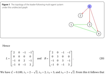
Figure 1The topology of the leader-following multi-agent system under the undirected graph

Hence

L=

⎡ ⎢ ⎢ ⎢ ⎣

2 0 –1 –1

0 0 0 0

–1 0 2 –1

–1 0 –1 2

⎤ ⎥ ⎥ ⎥

⎦ and B= ⎡ ⎢ ⎢ ⎢ ⎣

2 0 –1 –1

0 3 0 0

–1 0 3 –1

–1 0 –1 3

⎤ ⎥ ⎥ ⎥

⎦. (20)

We haveL= 0.100,λ1= 2 –√2,λ2= 2,λ3= 3, andλ4= 2 +√2. From this it follows that

λmin=min{λ1,λ2,λ3,λ4} ≈0.585 and

max1 – 0.462·0.250·0.585,e–0.585≤max{0.933, 0.557}= 0.933 =:M.

From the above we get

s∈Ts

M+μ∗L≈ s∈Ts

0.983 = 0

and

lim i→∞e

sum(i)_≈ _lim i→∞e

i

j=3(0.108j–3–0.070·0.250(i–2–2i–3+i–6))_<∞_.

All assumptions of Corollary1are satisﬁed, and thus equation (5) is exponentially stable. System (2)–(3) achieves consensus exponentially.

In Example4we have

lim i→∞e

LM–1i

j=1(T2j–T2j–1)≈ _lim

i→∞e

0.108ij=3j–3_<∞_,

but this condition is not required for the exponential stability of (5) (see Example5).

Remark2 If conditions (7)–(9), (12), and (18) are satisﬁed and if

γ(t)≡γ ∈R (21)

and

LM–1₊_γ_ln_M_{< 0,} ₍₂₂₎

(14)

Proof If condition (21) holds, then

sum(i) =

i

j=1

LM–1₍_T

2j–T2j–1) +γ(T2j–T2j–1)lnM

=LM–1+γlnM i

j=1

(T2j–T2j–1).

By (22) we see thatsum(i) < 0 for anyi∈Nandesum(i) _{is a positive decreasing function}

of the variable i∈N. Here_s_∈_Ts(M+μ∗L) and esum(i) for any i∈Nare bounded. If

the cardinality of set Ts is inﬁnity, thenlims→∞

s∈Ts(M+μ∗L) = 0. If the cardinality

of set Td _{is inﬁnity, then} _lim

i→∞esum(i)= 0. Thus, by Theorem1, we obtain the

state-ment.

Example5 Let

T= ∞

i=3

i 2,

i 2+

1 i

.

HereTd₌∞ i=3[2i,

i 2+

1

i) andTs={ i 2+

1

i :i∈N,i≥3},

T0=T1= 1.500, T2≈1.833, T3= 2.000, . . . ,

μ(t) = 1 2–

t 2+

1 2

√

t2_{– 2} _for_t∈Ts_, _μ∗_{= 0.500.}

Moreover, let

f(t,x) = 0.250sinx

t2 , γ(t)≡2.000,

and let the matrixBbe given by (20) in equation (5). ThenL= 0.250,λmin≈0.585, and

max1 – 0.333·2.000·0.585,e–0.585≤max{0.390, 0.557}= 0.557 =:M.

Finally,

LM–1₊_γ_ln_M_≈_{0.449 – 1.170 = –0.721 < 0.}

All assumptions of Remark2hold, and thus equation (5) is exponentially stable.

In Example5we have

lim i→∞e

LM–1i

j=1(T2j–T2j–1)_≈ _lim

i→∞e

0.449i_j₌₁1_i

=∞,

(15)

Corollary 2 If conditions(7)–(9)and(18)are satisﬁed and if ∞

i=0

(T2i+2–T2i+1) <∞, (23)

then equation(5)is exponentially stable.

Proof Since (23) holds,

esum(i)= constant.

Hence, recalling that the cardinality of the setTs_{is inﬁnity, by (}₁₈_{) we obtain}

lim i→∞e

sum(i) s∈[T0,T2i)∩Ts

M+μ∗L

=lim i→∞c

∗

s∈[T0,T2i)∩Ts

M+μ∗L

=c∗

s∈Ts

M+μ∗L= 0,

wherec∗=esum(i)_.

For two possible cases of carrying out of assumption (23), see Examples4and7. Theorem1generalizes Theorem 2 [14]. In the following example we present an equa-tion on time scale for which Theorem 2 [14] cannot be applied, but our Corollary2of Theorem1can be.

Example6 Let

T={i:i∈N} ∪

i+ 1

j+ 1:i,j∈N,j≥2 .

HereTd₌_{_i_:_i_∈_N}_and_Ts₌_{_i₊ 1

j+1:i,j∈N,j≥2},

T0= 1, T1=∞, μ(t) =

(t–i)2

1 +t–i fort∈T

s_, _μ∗_{= 0.500.}

Setf(t,x) = 0.250x,

γ(t) =

⎧ ⎨ ⎩ 1

μ(t) fort∈Ts,

0 fort∈Td,

andBis given by (20) in equation (5). We haveL= 0.250,λmin= 0.585, and

(16)

Hence

s∈Ts

M+μ∗L≈ s∈Ts

0.682 = 0.

All assumptions of Corollary2are satisﬁed, and thus equation (5) is exponentially stable.

Sincelim inft→∞μ(t) = 0, the results obtained in [14] cannot be applied.

The following examples show two different situations concerning time scale in which condition (23) is satisfied. In the first example,Td_{is a bounded set. In the second one,}_Td

is unbounded.

Example7 Let

T= [1, 2]∪[3, 7]∪ {n:n∈N,n≥8}.

HereTd= [1, 2]∪[3, 7] is bounded, andTs={n:n∈N,n≥8}. We see that

T0= 1, T1=T0= 1, T2= 2, T3= 3,

T4= 7, T5= 8, T6=∞,

μ(t) = 1 fort∈Ts, μ∗= 1.

Let also

f(t,x) = 1

4√tsinx, γ(t) =cost+ 2,

and let the matrixBbe given by (20) in equation (5). ThenL= 0.250,λmin= 0.585 and

M:=max1 – 1·1·0.585,e–0.585≈0.557 < 1.

As a consequence,

s∈Ts

M+μ∗L≈ s∈Ts

0.807 = 0.

All assumptions of Corollary2are satisﬁed, and thus equation (5) is exponentially stable. This means that the multi-agent system (2)–(3) achieves the leader-following consensus exponentially.

Example8 Let

T= ∞

i=3

i 2+

1 i+ 1,

i 2+

1 i

.

Here eitherTd₌∞ i=3[

i 2+

1 i+1,

i 2+

1 i) orT

s₌_{i 2+

1

i :i∈N,i≥3}is an unbounded set. We

see that

(17)

μ(t) = 1 2–

2

(t+√t2_{– 2)(2 +}_t₊√_t2_{– 2)} fort∈T

s_, _μ∗_{= 0.500.}

Moreover,

f(t,x) = x

4t, γ(t) = 1 4t

2_,

and the matrixBis given by (20) in equation (5). ThenL= 0.250,λmin= 0.585, and

max1 – 0.366·0.765·0.585,e–0.585< 0.836 =:M.

Hence

s∈Ts

M+μ∗L≈ s∈Ts

0.961 = 0.

All assumptions of Corollary2are satisﬁed, and thus equation (5) is exponentially stable. System (2)–(3) achieves consensus exponentially.

Notice that in Example8we have

lim i→∞e

LM–1i

j=1(T2j–T2j–1) = lim

i→∞e

0.299i_j₌₁_i₍_i1₊₁₎

=e0.299<∞.

Remark3 If conditions (7)–(9) are satisﬁed,

∞

j=1 T2j

T2j–1

γ(s)ds<∞,

and

lim i→∞e

LM–1i

j=1(T2j–T2j–1)·

s∈[T0,T2i)∩Ts

M+μ∗L= 0,

then equation (5) is exponentially stable.

(See Example4.)

Remark4 Let conditions (7)–(9) be satisﬁed. If the cardinality of the setTsis ﬁnite and sum(i) < 0 for anyi∈N, then equation (5) is exponentially stable.

Example9 Let

T={1} ∪ {11} ∪[12,∞).

HereTd_{= [12,}_∞_{) is an unbounded set, whereas}_Ts₌_{₁_{} ∪ {}₁₁_}_{is bounded, and}

(18)

Let

f(t,x) = 0.1x, γ(t) = 1,

and let the matrixBbe given by (20) in equation (5). ThenL= 0.100,λmin≈0.585, and

max1 – 0.585,e–0.585< 0.557 =:M.

Hence

sum(i)≈0.180(T2–T1) – 0.585 T2

T1

ds= –0.405(T2–T1) = –∞< 0.

All assumptions of Remark4are satisﬁed, and thus equation (5) is exponentially stable.

Notice that in Example9condition (18) does not hold.

Acknowledgements

Not applicable.

Funding

Ewa Schmeidel was supported by the Polish National Science Center grant on the basis of decision

DEC-2014/15/B/ST7/05270. Urszula Ostaszewska and Małgorzata Zdanowicz have been supported by the Polish Ministry of Science and Higher Education under a subsidy for maintaining the research potential of the Faculty of Mathematics and Informatics, University of Bialystok.

Availability of data and materials

Not applicable.

Competing interests

The authors declare that they have no competing interests.

Authors’ contributions

The main idea of this paper comes from Ewa Schmeidel. Proofs of theorems and examples are the joint work of all coauthors. All authors read and approved the ﬁnal manuscript.

Publisher’s Note

Springer Nature remains neutral with regard to jurisdictional claims in published maps and institutional aﬃliations.

Received: 20 April 2019 Accepted: 28 May 2019 References

1. DeGroot, M.H.: Reaching a consensus. J. Am. Stat. Assoc.69, 118–121 (1974).https://doi.org/10.1080/01621459

2. Krause, U.: A discrete nonlinear and non-autonomous model of consensus formation. In: Communications in Diﬀerence Equations. ICDEA, vol. 1998. Gordon & Breach, Pozna ´n (2000).https://doi.org/10.1109/IYCE.2015.7180798

3. Hegselmann, R., Krause, U.: Opinion dynamics and bounded conﬁdence: models, analysis, and simulation. J. Artif. Soc. Soc. Simul.5, 1–33 (2002)

4. Jadbabaie, A., Lin, J., Morse, A.S.: Coordination of groups of mobile autonomous agents using nearest neighbor rules. IEEE Trans. Autom. Control48(6), 988–1001 (2003).https://doi.org/10.1109/TAC.2003.812781

5. Blondel, V.D., Hendrickx, J.M., Tsitsikli, J.N.: On Krause’s multi-agent consensus model with state-dependent connectivity. IEEE Trans. Autom. Control54(11), 2586–2597 (2009).https://doi.org/10.1109/TAC.2009.2031211

6. Blondel, V.D., Hendrickx, J.M., Tsitsikli, J.N.: Continuous-time average-preserving opinion dynamics with opinion-dependent communications. SIAM J. Control Optim.18(8), 5214–5240 (2010).

https://doi.org/10.1137/090766188

7. Girejko, E., Machado, L., Malinowska, A.B., Martins, N.: Krause’s model of opinion dynamics on isolated time scales. Math. Methods Appl. Sci.39(18), 5302–5314 (2016).https://doi.org/10.1002/mma.3916

8. Girejko, E., Malinowska, A.B., Schmeidel, E., Zdanowicz, M.: The emergence on isolated time scales. In: 21st International Conference on Methods and Models in Automation and Robotics (MMAR), IEEExplore (2016).

https://doi.org/10.1109/MMAR.2016.7575317

9. Cucker, F., Smale, S.: On the mathematics of emergence. Jpn. J. Math.2(1), 197–227 (2007).

(19)

10. Cucker, F., Smale, S.: Emergent behavior in ﬂocks. IEEE Trans. Autom. Control52(7), 852–862 (2007).

https://doi.org/10.1109/TAC.2007.895842

11. Girejko, E., Machado, L., Malinowska, A.B., Martins, N.: On consensus in the Cucker–Smale type model on isolated time scale. Discrete Contin. Dyn. Syst., Ser. B11(1), 77–89 (2018).https://doi.org/10.3934/dcdss.2018005

12. Wang, Y., Cheng, L., Wang, H., Hou, Z.G., Tan, M., Yu, H.: Leader-following consensus of discrete-time linear multi-agent systems with communication noises. In: 34th Control Conference (CCC), Hangzhou, China. Lecture Notes in Electrical Engineering, vol. 407. IEEE, New York (2015).https://doi.org/10.1109/ChiCC.2015.7260748

13. Ostaszewska, U., Schmeidel, E., Zdanowicz, M.: Leader-following consensus on discrete time scales. In: ICNAAM 2017, Thessaloniki, Greece. AIP Conference Proceedings. American Institute of Physics, New York (2018).

https://doi.org/10.1063/1.5044162

14. Ostaszewska, U., Schmeidel, E., Zdanowicz, M.: Emergence of consensus of multi-agents systems on time scales. Miskolc Math. Notes (to appear)

15. Aulbach, B., Hilger, S.: A uniﬁed approach to continuous and discrete dynamics. In: Qualitative Theory of Diﬀerential Equations (Szeged, 1988). Colloq. Math. Soc. Jámos Bolyai, vol. 53. North-Holland, Amsterdam (1990)

16. Bohner, M., Peterson, A.: Dynamic Equations on Time Scales. Birkhäuser, Boston (2001).

https://doi.org/10.1109/IYCE.2015.7180798

17. Bohner, M., Peterson, A.: Advances in Dynamic Equations on Time Scales. Birkhäuser, Boston (2003)

18. Yu, Z., Jiang, H., Hu, C.: Leader-following consensus of fractional-order multi-agent systems under ﬁxed topology. Neurocomputing149, 613–620 (2015).https://doi.org/10.1016/j.neucom.2014.08.013

19. Schmeidel, E.: The existence of consensus of a leader-following problem with Caputo fractional derivative. Opusc. Math.39(1), 77–89 (2019).https://doi.org/10.7494/OpMath.2019.39.1.77

20. Berezansky, L., Migda, M., Schmeidel, E.: Some stability conditions for scalar Volterra diﬀerence equations. Opusc. Math.36(4), 459–470 (2016).https://doi.org/10.7494/OpMath.2016.36.4.459

21. Elaydi, S.N.: An Introduction to Diﬀerence Equations. Springer, New York (2005)

22. Peterson, A., Raﬀoul, Y.N.: Exponential stability of dynamic equations on time scales. Adv. Diﬀer. Equ.2005, 858671 (2005).https://doi.org/10.1155/ADE.2005.133

23. Bodine, S., Lutz, D.A.: Exponential functions on time scales: their asymptotic behavior and calculation. Dyn. Syst. Appl.