R E S E A R C H
Open Access
Convergence and stability of the
compensated split-step
θ
-method for
stochastic differential equations with jumps
Jianguo Tan
1*, Zhiming Mu
2and Yongfeng Guo
1*Correspondence: [email protected] 1Department of Mathematics, Tianjin Polytechnic University, Tianjin, 300387, P.R. China Full list of author information is available at the end of the article
Abstract
In this paper, we develop a new compensated split-step
θ
(CSSθ) method for stochastic differential equations with jumps (SDEwJs). First, it is proved that the proposed method is convergent with strong order 1/2 in the mean-square sense. Then the condition of the mean-square (MS) stability of the CSSθmethod is obtained. Finally, some scalar test equations are simulated to verify the results obtained from theory, and a comparison between the compensated stochastic theta (CST) method by Wang and Gan (Appl. Numer. Math. 60:877-887, 2010) and CSSθis analyzed. Meanwhile, the results show the higher efficiency of the CSSθmethod.Keywords: stochastic differential equations; Poisson jumps; compensated split-step
θ
-method; convergence; mean-square stability1 Introduction
In this paper, we consider one-dimensional Itô stochastic differential equations (SDEs) with Poisson-driven jumps
dX(t) =fXt–dt+gXt–dW(t) +hXt–dN(t) (.)
fort> , withX(–) =X, whereX(t–) denotes lim
s→t–X(s),f :R→R,g:R→R,h:
R→R,W(t) is a scalar standard Wiener process, andN(t) is a scalar Poisson process with intensityλ.
Recently, stochastic differential equations with jumps (SDEwJs) are becoming increas-ingly used to model real-world phenomena in different fields, such as economics, finance, biology, and physics. However, few analytical solutions have been proposed so far; thus, it is necessary to develop numerical methods for SDEwJs and study the properties of these methods. For example, Higham and Kloeden [] studied the convergence and stability of the implicit method for jump-diffusion systems, and they further analyzed the strong con-vergence rates of the backward Euler method for a nonlinear jump-diffusion system []. Chalmers and Higham [] studied the convergence and stability for the implicit simula-tions of SDEs with random jump magnitudes. Higham and Kloeden [] constructed the split-step backward Euler (SSBE) method and the compensated split-step backward Euler (CSSBE) method for nonlinear SDEwJs. Bruti-Liberati and Platen [, ] developed strong and weak approximations of SDEwJs.
Lately, Wang and Gan [] started to focus on the CST method for stochastic differential equations with jumps. Hu and Gan [] studied the convergence and stability of the bal-anced methods for SDEwJs. The split-stepθ (SSθ) method was firstly developed by Ding
et al.[] to solve the stochastic differential equations. Thus, we will construct the com-pensated split-stepθ method (CSSθ) for SDEwJs.
In this paper, we investigate the convergence and mean-square stability of the CSSθ method for SDEwJs. The outline of the paper is as follows. In Section , we introduce some notations and hypotheses and give the CSSθ method for SDEwJs. In Section , we prove that the numerical solutions produced by the CSSθmethod converge to the true solutions with strong order /. In Section , the mean-square stability of the CSSθ method for linear test equation is studied. At last, some numerical experiments are used to verify the results obtained from the theory.
2 The compensated split-step
θ
-methodFor the existence and uniqueness of the solution for (.), we usually assume thatf,g, and
hsatisfy the following assumptions:
(H) (The uniform Lipschitz condition) There is a constantK> , for allx,y∈R, such that
f(x) –f(y)
∨g(x) –g(y)∨h(x) –h(y)≤K|x–y|. (.)
(H) (The linear growth condition) There is a constantL> , for allx∈R, such that
f(x)∨g(x)∨h(x)≤L +x. (.)
We assume that the initial dataE|X()|is finite andX() is independent ofW(t) and
N(t) for allt≥. Under these conditions, we note that equation (.) has a unique solution on [, +∞), see [, ].
For a constant step sizeh=t> , we first define the split-stepθ(SSθ) method for (.) byY=X(–) and
Yn∗=Yn+
( –θ)f(Yn) +θf
Yn∗
t, (.)
Yn+=Yn∗+g
Yn∗
Wn+h
Yn∗
Nn, (.)
whereθ ∈[, ],Ynis the numerical approximation ofX(tn) withtn=n·t. Moreover,
the incrementsWn:=W(tn+) –W(tn) are independent Gaussian random variables with
mean and variancet;Nn:=N(tn+) –N(tn) are independent Poisson distributed
ran-dom variables with meanλtand varianceλt.
If we giveθ = , the SSθ method becomes the SSBE method in []. Ifθ = , the SSθ method is an explicit method.
Note that the compensated Poisson process
˜
N(t) :=N(t) –λt,
which is a martingale. Defining
we can rewrite the jump-diffusion system (.) in the form
dX(t) =fλ
Xt–dt+gXt–dW(t) +hXt–dN˜(t). (.)
We note thatfλalso satisfies the uniform Lipschitz condition and linear growth condition with larger constants
Kλ= (λ+ )K, Lλ= (λ+ )L. (.)
Then we define the compensated split-stepθmethod (CSSθ) for (.) byY=X(–) and
Yn∗=Yn+
( –θ)fλ(Yn) +θfλ
Yn∗
t, (.)
Yn+=Yn∗+g
Yn∗
Wn+h
Yn∗
N˜n, (.)
whereN˜n:=N˜(tn+) –N˜(tn).
If we giveθ= , the CSSθmethod becomes the CSSBE method in [].
To answer the question of the existence of numerical solution, we will give the following lemma.
Lemma . Assume that f :R→Rsatisfies(.),and let <θ< , <t< /(√Kλθ),
then equation(.)can be solved uniquely for Yn∗,with probability.
Proof Writing (.) asYn∗=F(Yn∗) =a+θ tfλ(Yn∗),a∈R, and using condition (.), we
have
F(u) –F(v)=θ tfλ(u) –θ tfλ(v) ≤Kλθ t|u–v|.
Then the result follows from the classical Banach contraction mapping theorem [].
3 Strong convergence on a finite time interval[0,T]
In this section, we prove the strong convergence of the CSSθmethod for problem (.) on a finite time interval [,T], whereTis a constant.
When Lemma . is followed, we find it is convenient to use continuous-time approxi-mation solution in our strong convergence analysis. Hence, fort∈[tn,tn+), we can define
the two step-functions:
Z(t) =
N–
n=
YnI[nt,(n+)t)(t), (.)
Z(t) =
N–
n=
Yn∗I[nt,(n+)t)(t), (.)
whereNis the largest number such thatNt≤T, andIAis the indicator function for the
Whent∈[tn,tn+), Lemma . ensures the existence ofYn∗by (.), then we define
Thus we can rewrite (.) in the integral form as follows:
Y(t) =Y+ crete solutions at the gridpoints. Hence we refer toY(t) as a continuous-time extension of the discrete approximation{Yn}. So our plan is to prove a strong convergence result for
Y(t).
Now we begin the proof of the strong convergence of the CSSθmethod, our first lemma shows the relationship betweenE|Yn∗|andE|Yn|.
Proof Squaring both sides of (.), we find
Due tot< , linear growth condition (.), and <θ< , we can get
Taking mathematical expectation for both sides, we can obtain
EYn∗≤
produced by the CSSθ method, have bounded second moments.
Lemma . Under conditions(.)-(.),let Ynand Yn∗ (n= , , . . . ,N)be produced by
where Cand Care two positive constants independent oft.
Squaring both sides, taking the mathematical expectation and using the element
in-Using the martingale isometry and linear growth condition (.), we have
E so we use the isometry
(see, for example, []), then we have
Inserting (.)-(.) in (.) gives
E|Yn+|≤
By Lemma ., we can derive that
E|Yn+|≤
Then, using the discrete Gronwall inequality, we can get
E|Yn|≤cec≡C.
Then, by Lemma ., we can obtain that
EYn∗
≤AE|Yn|+B≤AC+B≡C.
The next lemma shows that the continuous-time approximationY(t) in (.) remains close to the step functionsZ(t) andZ(t) in the mean square sense.
Lemma . Under conditions(.)-(.),let Yn∗ and Ynbe produced by(.)and(.),
and let <θ< , <t<min{, θLλ,
√
Kλθ},then there exist two positive constants Cand Cthat are independent oft,such that
EY(t) –Z(t)≤Ct, (.)
and
EY(t) –Z(t)
≤Ct, (.)
where t∈[,T],Z(t),Z(t),and Y(t)are defined by(.), (.), (.),respectively.
Proof For anyt∈[,T], there exists a nonnegative integernsuch that
t∈nt, (n+ )t⊆[,T],
we have
Y(t) –Z(t) =Y(t) –Yn
=
t nt
( –θ)fλ
Z(s)+θfλ
Z(s)ds
+
t nt
gZ(s)
dW(s)
+
t nt
hZ(s)dN˜(s).
Squaring both sides and using the element inequality (a+b+c)≤|a|+ |b|+ |c|, we have
Y(t) –Z(t)≤
t nt
( –θ)fλ
Z(s)+θfλ
Z(s)ds
+
t nt
gZ(s)dW(s)
+
t nt
hZ(s)
dN˜(s)
Taking mathematical expectation, by the element inequality (a+b)≤|a|+ |b|, and using the martingale isometry, we have
EY(t) –Z(t)
By the linear growth conditions (.) and (.), we get
EY(t) –Z(t)≤tLλ
Taking mathematical expectation, and by the linear growth condition (.),
Then by Lemma . we can derive
EZ(t) –Z(t)≤Lλ( +C+C)t. (.)
Then, by the element inequality (a+b)≤|a|+ |b| and using (.) and (.), we have
EY(t) –Z(t)
≤EY(t) –Z(t)
+ EZ(t) –Z(t)
≤Ct+ Lλ( +C+C)t ≤Ct,
whereC= C+ Lλ( +C+C). Then we have proved (.).
Now we use the above lemmas to prove a strong convergence result.
Definition . A numerical method is said to have strong order of convergence equal to γ if there exists a constantCsuch that the numerical solution sequenceYnproduced by
this numerical scheme satisfies
EYn–X(τ)≤Ctγ
for any fixedτ=nt∈[,T], andtsufficiently small.
Theorem . Under conditions(.)-(.),let <θ< , <t<min{, θLλ,
√
Kλθ},the continuous-time approximate solution Y(t)defined by(.)will converge to the true solu-tion of(.)in the mean square sense,i.e.,
E sup ≤t≤T
Y(t) –X(t)≤Ct, (.)
where Cis a positive constant independent oft.
Proof From (.) and (.), we have
Y(t) –X(t)
=
t
( –θ)fλ
Z(s)–fλ
Xs–+θfλ
Z(s)–fλ
Xs–ds
+
t
gZ(s)–gXs–dW(s) +
t
hZ(s)–gXs–dN˜(s). (.)
For any t∈[,T], using the Cauchy-Schwarz inequality and the inequality |θx+ ( – θ)y|≤θ|x|+ ( –θ)|y|, we have
E sup ≤t≤t
Y(t) –X(t)
≤E sup
≤t≤t
t
( –θ)fλ
Z(s)
–fλ
+θfλ
Now using the Doob martingale inequality for the two martingale terms, we have
E sup
Then Fubini’s theorem and the martingale isometries give
E sup
Applying Lipschitz conditions (.) and (.), we get
= TKλ
t
EZ(s) –Xs–ds
+ (TKλ+ K+ λK)
t
EZ(s) –X
s–ds
≤TKλ
t
EZ(s) –Ys–+EY(s) –Xs–ds
+ (TKλ+ K+ λK)
t
EZ(s) –Ys–+EY(s) –Xs–ds.
Finally, applying Lemma ., we have
E sup ≤t≤t
Y(t) –X(t)
≤TKλCt+ (TKλ+ K+ λK)TCt
+ (TKλ+TKλ+ K+ λK)
t
EY(s) –Xs–ds
≤TKλCt+ (TKλ+ K+ λK)TCt
+ (TKλ+ K+ λK)
t
E sup ≤r≤s
Y(r) –Xr–ds. (.)
Using the Gronwall inequality (see []), we have
E sup ≤t≤t
Y(t) –X(t)
≤Ct. (.)
Thus for anyt∈[,T], we have
E sup ≤t≤T
Y(t) –X(t)≤Ct. (.)
4 Mean-square stability
In order to study the stability property of the CSSθmethod, we consider a linear test equa-tion with scalar coefficients
dX(t) =aXt–dt+bXt–dW(t) +cXt–dN(t), (.)
wherea,b,c∈R. Hence, the mean-square stability of the zero solution to equation (.) was proved in [],i.e.,
lim
t→∞EX(t)
= ⇔ a+b+λc(c+ ) < . (.)
Applying the CSSθmethod (.)-(.) to equation (.), we have
Yn∗=Yn+
( –θ)(a+λc)Yn+θ(a+λc)Yn∗
h, (.)
Definition . Under condition (.), a numerical method applied to equation (.) is said to be MS-stable if there existsh(a,b,c,λ) > such that the numerical solution sequence
Ynproduced by this numerical scheme satisfies
lim
n→∞E|Yn|
= (.)
for allh∈(,h(a,b,c,λ)).
Theorem . Under condition(.),then for
t≤h(a,b,c,λ,θ) =–B+ √
B– AC
A , (.)
where
A= ( –θ)(a+λc)b+λc,
B= ( – θ)(a+λc)+ ( –θ)(a+λc)b+λc,
C= a+b+λc(c+ ),
θ∈[, ),
the CSSθmethod(.)-(.)applied to equation(.)is MS-stable.
Proof Assuming that –θ(a+λc)h= , from (.) we have
Yn∗=
+ ( –θ)(a+λc)h
–θ(a+λc)h Yn. (.)
Substituting this into (.) yields
Yn+=
+ ( –θ)(a+λc)h
–θ(a+λc)h ( +bWn+cN˜n)Yn. (.)
Squaring both sides of (.), we can get
|Yn+|=
+ ( –θ)(a+λc)h
–θ(a+λc)h
( +bWn+cN˜n)|Yn|. (.)
Noting thatE(Wn) = ,E[(Wn)] =h,E(N˜n) = ,E[(N˜n)
] =λh, we have
E|Yn+|=
+ ( –θ)(a+λc)h
–θ(a+λc)h
+bh+λchE|Yn|. (.)
By the iteration of (.), we conclude thatlimn→∞E|Yn|= if
+ ( –θ)(a+λc)h
–θ(a+λc)h
which is equivalent to
+ ( –θ)(a+λc)h +bh+λch< –θ(a+λc)h, (.)
i.e.,
( –θ)(a+λc)b+λch
+( – θ)(a+λc)+ ( –θ)(a+λc)b+λch
+ a+b+λc(c+ ) < . (.)
Let
f(h) =( –θ)(a+λc)b+λch
+( – θ)(a+λc)+ ( –θ)(a+λc)b+λch
+ a+b+λc(c+ ). (.)
Ifθ= , (.) becomes
–(a+λc)h+ a+b+λc(c+ ) < . (.)
By (.), we know that (.) holds for allh> ,i.e., the CSSθmethod is MS-stable for all
h> . Note that ifθ = , the CSSθ method reduces to CSSBE, and (.) coincides with Theorem which was studied in [].
Ifθ∈[, ), let
A= ( –θ)(a+λc)b+λc,
B= ( – θ)(a+λc)+ ( –θ)(a+λc)b+λc,
C= a+b+λc(c+ ).
(.)
In view of (.), we know thata+λc< , thenA= (ifA= ,b+λc= ,i.e.,b= ,c= , then equation (.) becomes nonsense), so we can get
A> ,
B= ( – θ)(a+λc)+ ( –θ)(a+λc)b+λc
< ( – θ)(a+λc)– ( –θ)(a+λc)(a+ λc)
= (– + θ)(a+λc)< ,
C< ,
=B– AC> .
Sof(h) = has two real rootshandh, withh< <h, where
h(a,b,c,λ,θ) =–B+ √
A > ,
h(a,b,c,λ,θ) =–B– √
A < .
(.)
So we can easily obtain thatf(h) < holds when
h∈,h(a,b,c,λ,θ).
From (.), we know that the CSSθmethod is MS-stable. This proves the theorem.
5 Numerical experiments
We consider the following equation:
dX(t) =aX(t–) dt+bX(t–) dW(t) +cX(t–) dN(t),
X() = . (.)
Equation (.) has the exact solution
X(t) =X()exp
a–
b
t+bW(t)
( +c)N(t), (.)
see, for example, [].
To illustrate the convergence order and the linear mean-square stability of the CSSθ method, we choose the following examples from the reference [].
Example . a= –,b= ,c= ,λ= .
Example . a= ,b= ,c= –.,λ= .
In this section, the data used in all figures are obtained by the mean square of data by , trajectories, that is,ωi: ≤i≤,,Yn= /,
,
i= |Yn(ωi)|; in all figurestn
denotes the mesh-point.
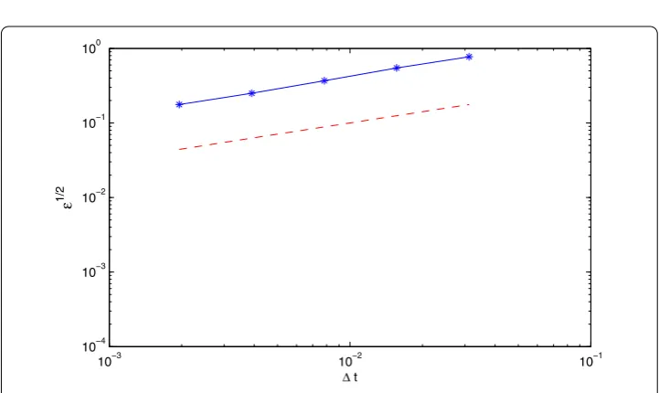
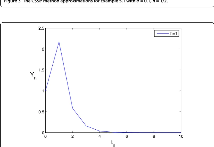
To show the strong convergence order of the CSSθmethod, we apply the CSSθmethod to Example .. First, we plot the exact solution of Example . for one sample path and the CSSθ approximations in Figure . Then we simulate the numerical solutions with five different step sizes h= p–t for ≤p≤, t= –. The mean-square errors ε= /,,i= |Yn(ωi) –X(T)|all measured at timeT= are estimated by trajectory
averaging. We plot our approximation to√ againstton a log-log scale. For reference a dashed line of slope one-half is added. We see that the slopes of the two curves appear to match well in Figure . Hence, our results are consistent with a strong order of conver-gence equal to /.
Figure 1 The exact solution and the CSSθmethod approximations with fixedθ= 0.1 for Example 5.1.
Figure 2 The convergence rate of the CSSθmethod for Example 5.1 with fixedθ= 0.2.
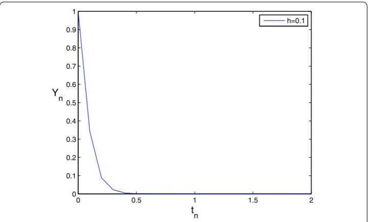
For Example ., we first chooseθ = ., then by Theorem . we know that the CSSθ method is MS-stable whenh(a,b,c,λ,θ) = .. Figure illustrates the numerical so-lution produced by the CSSθ method is MS-stable whenh= /. However, applied to the same test equation, and also chooseθ= ., then by Theorem . in [] the CSTM is MS-stable when the step sizeh∈(, .).
When we chooseθ= ., by Theorem . we know that the CSSθmethod is MS-stable whenh(a,b,c,λ,θ) = ., while the CST method in [] is MS-stable when the step size
Figure 3 The CSSθmethod approximations for Example 5.1 withθ= 0.1,h= 1/2.
Figure 4 The CSSθmethod approximations for Example 5.1 withθ= 0.4,h= 1.
Remark Figures and indicate that the restriction on the step sizehof the CSSθ method for the MS-stability is less than that of both the CST method and the EM method.
Figure 5 The CSSθmethod approximations for Example 5.2 withθ= 0.1,h= 0.1.
Figure 6 The CSSθmethod approximations for Example 5.2 withθ= 0.4,h= 0.5 (upper),h= 0.6 (lower).
At last, Figure (lower) shows that the numerical solution of the CSSθ method is still stable whenh= . >h(a,b,c,λ,θ) = .. This implies that maybe the mean-square stability bound we obtained by Theorem . is not optimal.
Competing interests
The authors declare that they have no competing interests. Authors’ contributions
All the authors contributed equally to this work. They all read and approved the final version of the manuscript. Author details
Acknowledgements
This research was supported with funds provided by the National Natural Science Foundation of China (Nos. 11226321, 11272229 and 11102132). We thank two anonymous reviewers for their very valuable comments and helpful suggestions which improved this paper significantly.
Received: 27 December 2013 Accepted: 8 July 2014 Published:04 Aug 2014
References
1. Higham, DJ, Kloeden, PE: Convergence and stability of implicit methods for jump-diffusion. Int. J. Numer. Anal. Model.
3, 125-140 (2006)
2. Higham, DJ, Kloeden, PE: Strong convergence rates for backward Euler on a class of nonlinear jump-diffusion problems. J. Comput. Appl. Math.205, 949-956 (2007)
3. Chalmers, GD, Higham, DJ: Convergence and stability analysis for implicit simulations of stochastic differential equations with random jump magnitudes. Discrete Contin. Dyn. Syst., Ser. B9, 47-64 (2008)
4. Higham, DJ, Kloeden, PE: Numerical methods for nonlinear stochastic differential equations with jumps. Numer. Math.101, 101-119 (2005)
5. Bruti-Liberati, N, Platen, E: On the weak approximation of jump-diffusion processes. Technical report, University of Technology Sydney, Sydney (2006)
6. Bruti-Liberati, N, Platen, E: Strong approximations of stochastic differential equations with jumps. J. Comput. Appl. Math.205, 982-1001 (2007)
7. Wang, XJ, Gan, SQ: Compensated stochastic theta methods for stochastic differential equations with jumps. Appl. Numer. Math.60, 877-887 (2010)
8. Hu, L, Gan, SQ: Convergence and stability of the balanced methods for stochastic differential equations with jumps. Int. J. Comput. Math.88, 2089-2108 (2011)
9. Ding, XH, Ma, Q, Zhang, L: Convergence and stability of the split-stepθ-method for stochastic differential equations. Comput. Math. Appl.60, 1310-1321 (2010)
10. Gikhman, II, Skorokhod, AV: Stochastic Differential Equations. Springer, Berlin (1972)
11. Sobczyk, K: Stochastic Differential Equations with Applications to Physics and Engineering. Kluwer Academic, Dordrecht (1991)
12. Smart, DR: Fixed Point Theorems. Cambridge University Press, Cambridge (1974)
13. Gardon, A: The order of approximation for solutions of Itô-type stochastic differential equations with jumps. Stoch. Anal. Appl.22, 679-699 (2004)
14. Mao, XR: Stochastic Differential Equations and Applications. Ellis Horwood, Chichester (1997) 15. Glasserman, P: Monte Carlo Methods in Financial Engineering. Springer, Berlin (2003)
10.1186/1687-1847-2014-209