Volume 2010, Article ID 430615,10pages doi:10.1155/2010/430615
Research Article
A Stochastic Multiobjective Optimization Framework for
Wireless Sensor Networks
Shibo He,
1Jiming Chen,
1, 2Weiqiang Xu,
1Youxian Sun,
1Preetha Thulasiraman,
2and Xuemin (Sherman) Shen
21State Key Lab of Industrial Control Technology, Zhejiang University, Hangzhou 310027, China
2Department of Electrical and Computer Engineering, University of Waterloo, Waterloo, ON, Canada N2L 3G1
Correspondence should be addressed to Xuemin (Sherman) Shen,[email protected]
Received 31 October 2009; Accepted 17 February 2010
Academic Editor: Yu Wang
Copyright © 2010 Shibo He et al. This is an open access article distributed under the Creative Commons Attribution License, which permits unrestricted use, distribution, and reproduction in any medium, provided the original work is properly cited.
In wireless sensor networks (WSNs), there generally exist many different objective functions to be optimized. In this paper, we propose a stochastic multiobjective optimization approach to solve such kind of problem. We first formulate a general multiobjective optimization problem. We then decompose the optimization formulation through Lagrange dual decomposition and adopt the stochastic quasigradient algorithm to solve the primal-dual problem in a distributed way. We show theoretically that our algorithm converges to the optimal solution of the primal problem by using the knowledge of stochastic programming. Furthermore, the formulation provides a general stochastic multiobjective optimization framework for WSNs. We illustrate how the general framework works by considering an example of the optimal rate allocation problem in multipath WSNs with time-varying channel. Extensive simulation results are given to demonstrate the effectiveness of our algorithm.
1. Introduction
The layered architecture approach has achieved great success in traditional wired network design by dividing the whole architecture into several modules, called layers, each of which performs a separate functionality. As each layer design only needs some interface variables from the layer below, the com-plexity of other layers can be hidden. The layered architecture approach suggests that the network design can be scalable, evolvable, and implementable. However, it may have limita-tions in improvement of efficiency and fairness, and suffer potential risks of manageability [1], which motivates the optimization of network design. Chiang et al. [1,2] propose an optimization decomposition technique to systematically understand the network architecture, known as “layering
as optimization decomposition”. They model the network as
an optimization problem and decompose the problem into many subproblems. They classify the decompositions into
vertical decompositionandhorizontal decomposition.Vertical
decomposition layers the network architecture into several
modules and horizontal decompositionprovides distributed algorithms to fulfill the functionality within the modules.
According to the requirements of the applications, the decomposition may be different, yielding different layers and distributed algorithms. There are usually two steps in the process of layering as optimization decomposition: (1) modeling the network problem as a specific NUM problem, and (2) exploring the alternative decompositions to design different modules and distributed algorithms. Most existing efforts have been put to the second step and simply assume that the network problems can be modeled by a unified utility function at the first step [3–6]. However, not all net-work problems can be modeled by a unified utility function in a tractable way since there may exist many objectives to be achieved, such as guaranteeing fairness, maximizing throughput, reducing packet dropping and delay, prolonging the network lifetime, and so forth. It may not be possible to integrate all these objectives into a single unified utility function, that is, network problems should be formulated as multiobjective optimization problems.
application from scratch, the implementation can hardly be transplantable to other applications. This is especially aggravated in wireless sensor networks (WSNs) due to the application-oriented and infrastructureless nature of these networks. For example, if we design an efficient algorithm for events monitoring, the network lifetime is the main concern and the propagation delay can be tolerant, but it is difficult to apply such algorithm to online query applications, where the query delay is the primary objective.
In this paper, we utilize the concept of multiobjective optimization and provide a general framework for a specific class of applications in WSNs. It is well known that the TCP/IP reference model, one of the most popular layered architectures, divides the whole architecture into five layers (modules), and each layer only communicates with the layers next to it, while recent work on the NUM approach divides the architectures according to applications. We first list all the constraints and objectives which the applications may have. Then the network architecture is divided inton
modules, each of which has several interface variables with other modules. In this way, we can inherit the advantages of both the layered architectures (as we have fixed modules) and the NUM approach (as each module can communicate with other modules). We illustrate this inFigure 1, in which λandμare the interface variables (seeSection 3for detailed definition ofλandμ), andOiis the objective vector function in each modulei. We transform the objectives of the network into specific modules through the interface variables. Each sensor optimizes its own objective vector function to achieve the global optimal solution of the whole network. In this way, for different requirements from the network, we do not redesign the framework, that is, the modules and interfaces in Figure 1 can be kept unchanged. We only need to introduce multiobjective methods to optimize the vector functionOiin each module. This will greatly simplify network design for WSNs.
In WSNs, some parameters (e.g., the topology of the networks or channel condition) are time-varying. In [7], Lee et al. demonstrated that the state of the network can be more efficiently utilized to improve the performance of the network (e.g., increasing the throughput and reducing packet delay), by appropriately exploiting the variability of the time-varying channels. Also there are measurement errors in the implementation of distributed algorithms, such as the noisy feedback [8] or lossy links [9]. Therefore, we also characterize these random factors in our model. Our contributions in this paper are summarized as follows.
(1) We formulate a general multiobjective stochastic optimization problem for WSNs. We decompose the optimization problem through Lagrange dual decomposition and adopt the stochastic quasigra-dient method to solve the primal-dual problem. In other words, we transform the multiple objectives of WSNs into the multiple objectives of each individual sensor node. The global optimal solution can be obtained when each sensor node maximizes its own objective vector function. Therefore, our approach
Module 1,O1
Module 2,O2
Modulen,On . . . . . .
Figure1: An illustration of our proposed framework.
provides a general framework for multiobjective optimization for WSNs.
(2) We study the stability of the algorithm by using the knowledge of stochastic programming, and show that our algorithm for stochastic multiobjective optimiza-tion problem (ASMOP) can converge to the optimal solution of the primal problem.
(3) We demonstrate how the general framework can be applied to different applications, by considering the rate allocation problem as an example. We introduce three multiobjective optimization methods: (1) con-straint method, (2) linear weighted method, and (3) hierarchical sequence method. The three paradigms show that although different requirements may lead to different models [6,10], we can solve them in the general framework.
The remainder of the paper is organized as follows: in
Section 2, we discuss related work regarding the NUM
prob-lem and stochastic network utility maximization (SNUM). We formulate a general mathematical model and design a distributed algorithm to solve the problem inSection 3, and the stability of the algorithm is also discussed. We provide three paradigms in Section 4 to demonstrate the general framework for different applications. Simulation results are given inSection 5. We conclude the paper inSection 6.
2. Related Work
improve the throughput in multihop wireless networks [15]. Zhang et al. [8] elaborated on the impact of the feedback in the implementation of distributed NUM algorithms. Since feedback is often collected using error-prone measurement mechanisms, for example, biased estimator or unbiased estimator, they adopted the knowledge of stochastic approx-imation and proved stability of the algorithms of single-time scale and two-time scale. Lee et al. utilized the variation of channels to guide power and rate control in cross-layer design [7]. In this paper, we formulate a more general math-ematical model by considering stochastic multiple objectives in objective functions. We apply our approach to rate allocation problem in multipath WSNs with time-varying channels. Rate allocation is a fundamental problem and has been extensively investigated [16–19]. Low and Lapsley [16] first introduced the Lagrange dual method to decompose the problem and proposed two algorithms under synchronous and asynchronous scenarios. A multipath formulation for rate control in multi-cast networks was proposed in [20], and three distributed algorithms were proposed to solve the problem. The goal is to maximize the aggregate utility. In [6], Srinivasan et al. considered two objectives: utility maximization and guaranteeing prespecified network life-time for multipath wireless ad hoc networks. In [10], Zhu et al. also focused on the network lifetime and application performance (utility), and employed the linear weighted method from the multiobjective optimization to transform these two objective functions into a single one which was named to the utility-lifetime tradeofffunction.
3. General Multiobjective
Formulation and Solutions
Throughout the paper, we will denote sets by capital letters, variables by lowercase letters, vectors by bold lowercase letters, and matrices by bold capital letters. For a vectorx, we denote itsith component byxiand its transpose byxT. We use capital letters for both the sets and the cardinality of sets.
Consider S sensing nodes and N sink nodes in the region of interest. Let Ω be a probability space with a σ -algebraF of random events, and have a finite set{τm,m=
gs(·) a column vector function. We can formulate the primal problem (PP) as follows:
PP: P(x), In order to design a distributed algorithm, we introduce auxiliary variable y to decouple it. Assume that the node set associated with coupled variables of fs(i)(x) isH(i)(s),i= 1, 2,. . .,n. LetH(s)=n
i=1H(i)(s), which denotes the node
set associated with coupled variables ofPs(x) of sensing node
s, then the decoupled primal problem (DPP) can be given by
DPP: P x,y= P1 x,y,. . .,Pn x,y, (2)
vector of auxiliary variables.
In our formulation, the objective functions are determin-istic, taking the advantage that each sensing node can be obtained from the network. The constraint set contains the random factors of the networks, such as message exchange, and environmental effect. If we know the distribution,p(τm),
m = 1, 2,. . .,M, of τ, we can transform the problem into a deterministic one, by calculating the expectation. However, in WSNs, there is often no prior knowledge about the randomness from the networks themselves and the environmental effect. Therefore, we develop an algorithm without this prior knowledge, which can be achieved by the stochastic quasigradient method [7].
To decompose the problem, we take Lagrange dual approach. The Lagrange function [21] of (3) is given by
where Ps(xs,ys) is the objective vector function of sensing nodes. It is a formal expression which can be transformed into different objective functions for different applications.
coupling of objective functions). Since (4) is separable, we exploit the decomposable structure of Lagrangian function and decompose the problem intoSsubproblems. Maximiza-tion is achieved in each sensing node s, s ∈ S, with the knowledge of local variables (xs,ys) and the current stateτ, by solving the following optimization problemDPs.
DPs: max Ps xs,ys
−λT
gs(xs,τ)
+
⎛
⎝
s:s∈H(s)
uss
⎞ ⎠
T
xs−
s∈H(s)
uTssyss (5)
s.t. ⎧ ⎨ ⎩
xs∈χs,
yss∈χs.
(6)
At iterationt, each sensing node supdates its resource variablesxsand auxiliary variablesysaccording to
xs,ys
=Arg max
xs∈χs
yss∈χs
DPs.
(7)
We proceed to solve the dual problem. LetD(λ,μ,τ) =
maxx,yL(x,y,λ,μ,τ). Then the dual problem (DP) is given
by
min
λ≥0,μD λ,μ,τ
. (8)
At iterationt, each sensing node can acquire the state of random variablesτ. The stochastic quasigradient method only needs this current state information of the system and utilizes it to form the stochastic subgradients of D(λ,μ,τ) at iterationt. For the dual problem,DP, prices are updated according to
λ(t+ 1)=[λ(t)−α(t)ϑ(t)]+, (9) μss(t+ 1)=μss(t)−α(t)νss(t), s∈H(s), (10)
where ϑ(t) and νss(t) are the stochastic quasigradients of
D(λ,μ,τ).
In our algorithm, we set
α(t)=1
t, (11)
ϑ(t)= −
s∈S
g(xs(t),τ(t)), (12)
νss(t)=xs(t)−yss(t), s∈H(s), (13) whereτ(t) is the state ofτat iterationt.
We summarize our algorithm for the general formulation of stochastic multiobjective optimization problem (ASMOP) in theAlgorithm 1.
To prove that the algorithm can converge to the optimal solution of the primal problem, we make the following assumptions.
(1) fs(i)(·) as well as the objective vector functionPs(·) (which can be transformed into a single function in applications), s ∈ S, i = 1, 2,. . .,n, are twice continuous differentiable concave functions.
(2)gs(x,τ), s ∈ S, are convex and twice continuous differentiable functions inx, for allτ∈Ω.
Theorem 1. If(1)hold, then from an arbitrary point ofx(0)∈ χ, λ(0) ≥ 0 and yss(0) ∈ χss,μss(0),s ∈ S,s ∈ H(s),
the sequence generated by(7),(9), and(10)converges. Every
limit point(x∗,y∗,λ∗,μ∗)of the sequence(x(t),y(t),λ,μ)is
primal-dual optimal.
Proof. Let the sequences of iteration {λ(0),λ(1),. . .,λ(t)}
and {μ(0),μ(1),. . .,μ(t)} be generated by (9) and (10), respectively. Then to guarantee the convergence of the algorithm, according to [7, 22], the current stepsize and quasigradientsα(t),ϑ(t), andν(t) should be chosen such that
α(t)≥0, ∞
t=0
α(t)= ∞, ∞
t=0
(α(t))2<∞, (14)
Eϑ(t)|λ(0),. . .,λ(t),μ(0),. . .,μ(t)=∂λD λ(t),μ(t),τ(t), (15)
Eν(t)|λ(0),. . .,λ(t),μ(0),. . .,μ(t)=∂μD λ(t),μ(t),τ(t). (16)
It can be seen thatα(t)=1/n,t=0, 1,. . ., satisfy (14). From [22]; we know thatϑ(t) andνss(t) from (12) and (13) also satisfy (15) and (16).
From assumptions (1) and (2), the primal function is concave and the dual functionD is convex inλandμ for a fixedτ. From (7), (9), (10), (11), (12), and (13), we can conclude that the sequence converges to the optimal solution by solving the dual problem [22]. As the primal problem is a convex optimization problem, there is no gap between the primal and dual problems. So the sequence (x∗,y∗,λ∗,μ∗) generated by the algorithm is primal-dual optimal.
Remarks. Because of multipath routing, the problem,DPs,
may not be strictly concave even ifPs(·) is strictly concave. This may lead to oscillation of the sequences generated by the algorithms. There are several ways to cope with this problem. For example, we can first add some augmented variables to
DPsand adopt the first-order Lagrangian method to solve it [23].
solve the objective vector function independently according to different requirements.
4. Paradigms of Objective
Optimization in WSNs
In the proposed general framework, Ps(xs,ys) in DPs is a vector function and can be transformed into a single function according to different requirements. Therefore, solving DPs is application-dependent, which provides the flexibility of solving a class of applications by the general framework.
In this section, we consider the rate allocation problem as an example and show how the general framework works. Rate allocation problem is a well-investigated problem [24], and has different requirements for different applications. There are usually three methods to cope with the require-ments: (1) Constraint Method [6], (2) Linear Weighted Method [10], and (3) Hierarchical Sequence Method. While these methods are extensively studied in existing works, we can integrate these methods together into the general framework. Hence, our approach can be applied to a class of applications with different background, which will offer significant convenience to the designers.
4.1. Preliminary Knowledge. In this section, we give a brief
introduction to the three multiobjective methods.
(1) The constraint method tries to solve the multi-objective problems by placing the most important one in the objective function, while other objective functions are constrained within the constraint set. In other words, constraint method can solve the followingDPsof each sensing nodes. (without loss of generality, we assume thatfs(1)is the most important objective function)
(2) The linear weighted method focuses on solving the multiobjective optimization problems by first associ-ating each objective function fi(·) with a weightγi and then taking the weighted sum as a new objective function. Using linear weighted method to solveDPs,
the variables in each sensing node s are updated according to
(3) The hierarchical sequence method is concerned with solving the multiobjective optimization problems sequentially, that is, solving the most important problem first and then the less important problems. LetI= {x |xs∈χs,yss ∈χs}and divide (5) into
nfunctionsFj(xs,ys), j = 1, 2,. . .,n. Maximization is achieved by solving the followingnsubproblems sequentially.
4.2. Rate Allocation Problem under ASMOP Formulation. In
this section, we consider the rate allocation problem with two objectives: (1) maximizing aggregate utility and (2) prolonging the network lifetime.
Assume the sensing nodes can transmit their rates to the sink nodes over a setL= {1, 2,. . .,L}of links, each of which has capacitycl,l ∈ L. Each sensing nodescan transmit its rate throughR(s) ⊆ Rof the routes. Each router ∈ R(s) traverses over a set L(r) ⊆ L of links with a rate xsr. Let
xs be the rate vector of sensing node s, S(l) = {s ∈ S |
l ∈ L(r),r ∈ R(s)}the set of sensing nodes using link l, andR(s,l) the subset of routesR(s) used by sensing nodes
to traverse over linkl. We denote the set of sensing nodes that use sensing nodesas an interim relay node byS(s) (not including the sensing nodesitself). LetR(s,s) be the subset of routesR(s) which use sensing nodesas a relay node and
S(r) the relay nodes used by router. LetMbe finite number of state that the channels have and p(τm) the probability of the stateτm,m ∈ M. Each sensing nodesis characterized by three parameters (Us(·),bs,bs), whereUs:R+ → Ris a
From [11, 16], we know utility maximization can be the states of link channel condition andcm
l is the capacity of link l under state τm. We will establish algorithms that can guarantee convergence without prior knowledge of the underlying probability distribution of the system channel state.
The network lifetime is often defined as the time interval between initialization of the network and the exhaustion of the battery of the first sensing node. The total power dissipation,ws, at sensing nodesis equal to
ws=
sr andwre are the energy consumptions at sensing nodesfor transmitting or receiving unit data flow over route
r, respectively.
Let es denote the initial energy of sensing node s. Its lifetimeTsisTs=es/ws. Following [10], we have the energy model for the network lifetime:
max −
We can have the multiobjective model for rate allocation problem:
Here, parameter ω scales the values of the two objective functions into the same order of magnitude.
4.3. Algorithm Design. Similar to (3), the decoupled form of
(25) is
constraints (21), (22), (24), (29)
whereP(2)(x,y)= −
Then we have the Lagrange function:
L x,y,λ,μ,τ the update for each sensing nodesis deterministic, no matter what the channel condition is. So at iterationt, each sensing nodesupdates its ratexsand auxiliary variableysby solving the optimization below vector function for sensing nodes.
At iterationt,t=1, 2,. . ., sensing nodesfirst receivesλr,
μsr andμ
ssr,s ∈S(s),r ∈ R(s,s), from the network, and then updates its rate and auxiliary variables according to
xs(t),ys(t)=Arg maxDPs. (33) Notice that the update of decoupled prices, μ, does not depend on the channel condition. At each iterationt, with
xsr, yssr, s ∈ S(s), r ∈ R(s,s), being collected, the decoupled priceμis updated according to
μssr(t+ 1)=μssr(t)−α(t) xsr(t)−yssr(t). (34)
To update price λ, without prior knowledge about the distribution of the channel state, each sensing nodes can measure channel condition and get the link capacitycl(t) for each linklat timet. Thenλcan be updated according to
λl(t+ 1)=λ(t)−α(t)cl(t)−xl(t)+. (35)
4.4. Paradigms: Applications under Different Methods. (1) Constraint Method. To maximize the utility of a network under the condition that the network lifetime exceeds a prespecified threshold timeT, the constraint method can be used to solve the optimization problem below of each sensing nodes. considered the tradeoffbetween lifetime and rate allocation. By introducing the weight parameter, γ, to evaluate the importance of the two objectives, they can be combined into a single one. For (29), the desired tradeoff between network utility and lifetime can be achieved by solving the optimization problem below.
(3) Hierarchical Sequence Method. In our rate allocation paradigm, we have two objectives: (1) find a rate allocation strategy to maximize the total utility and (2) prolong the networks lifetime. To the best of our knowledge, this method has not been applied to the rate allocation problem before. We can achieve the two objectives by solving the two subproblems below sequentially.
Figure2: Topology of the simulated WSN.
It is sufficient to employ optimization methods to solve (37), (39), or (40), and (41) for different applications, while λandμupdates are kept unchanged (according to (34) and (35)).
5. Simulation Results
5.1. Simulation Setting. We use 9 sensing nodes and 1 sink
node in our simulations. These sensor nodes are randomly deployed in an area of size 70×70 to perform a sensing task. The randomly generated topology of the sensor nodes is shown in Figure 2, in which sensing nodes are marked by triangle icons and the sink node is marked by a square icon. In our simulations, we only focus on the rate allocation problem. The study of the routing in the network layer is beyond the scope of our paper. We assume that there are 15 routes available for data transmission.L(r1)= {l1,l5,l9},
We have two objectives: maximizing the aggregate utility and the network lifetime. For the utility objective, we set
Us(·) = ξslog(·) for each sensor node s, where ξ = (52, 54, 56, 58, 60, 62, 64, 66, 68). From [10], the function
−s(ω/(β − 1))z β−1
s can have a ratio higher than 0.95 to approximate the original lifetime problem T when
β ≥ 8. In our simulations, we use β = 9. The link capacities vary from time to time according to a uniform distribution with the expected capacities of links 1–13 to bec=(2000, 2000, 2200, 2000, 2000, 2500, 2800, 3500, 3500, 2000, 3000, 2800) (bit/s). For the energy consumption model, from [10], wre is a constant and w
0 5 10 15 20 25
×102
Rat
es
o
f
n
odes
(bit/s)
0 20 40 60 80 100
Iteration number (n) Node 1
Node 2
Node 3 Node 4 (a)
1 2 3 4 5 6 7 8 9 10
×102
Rat
es
o
f
n
odes
(bit/s)
0 20 40 60 80 100
Iteration number (n) Node 5
Node 6
Node 8 Node 9 Node 7
(b)
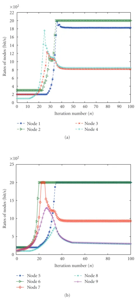
Figure 3: Convergence of the ASMOP algorithm by using con-straint method.
wheredsr is the length of the outgoing link of sensing node
s for transmitting rate of route r. We set ρ = 50 nJ/bit,
σ = 0.0013 pJ/bit/m4, η = 4, wre = 50 nJ/bit. The initial energy of the sensing nodes 1–9 is set to be e =
(450, 450, 475, 475, 450, 500, 500, 450, 500) (J) and the sink node (node 10) is assumed to have enough energy. The minimum and maximum rates of each sensing node are set to bebs=100 andbs=2500, respectively.
5.2. Simulation Results for Paradigms. First, we show the
per-formance of the ASMOP algorithm by using the constraint method. Let the threshold of the network lifetime T =
0 2 4 6 8 10 12 14 16 18 20 22
×102
Rat
es
o
f
n
odes
(bit/s)
0 10 20 30 40 50 60 70 80 90 100 Iteration number (n)
Node 1 Node 2
Node 3 Node 4 (a)
1 2 3 4 5 6 7 8 9 10 11
×102
Rat
es
o
f
n
odes
(bit/s)
0 20 40 60 80 100
Iteration number (n) Node 5
Node 6
Node 8 Node 9 Nods 7
(b)
Figure4: Convergence of the ASMOP algorithm by using linear weighted method.
800 h. We collect the rate of each router at each iteration. For each sensing node s, the rates are updated according to (37) and the decoupled priceμ is updated according to (34). Each linklfirst collects information about the channel condition and computes its corresponding capacity, then updates its link price according to (35). The results are shown
inFigure 3. Since there are 9 sensing nodes and 15 routes in
(1) Price update algorithm: At timest=1, 2,. . ., decoupled prices are updated according to λ(t+ 1)=[λ(t)−α(t)ϑ(t)]+
μss(t+ 1)=μss(t)−α(t)νss(t), s∈H(s),
(2) Sensor nodes’s Algorithm: At timet=1, 2,. . ., each sensing nodesupdates its variables according to
(xs,ys)=Arg maxx
s∈χs
yss∈χs
DPs
Algorithm1: ASMOP.
Next, we show the simulation results of the ASMOP algorithm using the linear weighted method. Here we set ω = 8.17 × 1026 and γ = 0.7. At each
itera-tion t, each sensing node s updates its rates according to (39), and the decoupled price λ and μ are updated as the same in paradigm I. The results are shown in
Figure 4, and similar conclusions can be made as in the
paradigm I.
A similar simulation is performed for the hierarchical sequence method and the corresponding results are shown
inFigure 5. We can see that the rates change sharply at the
beginning of each iteration, and then converge to the optimal one inFigure 5.
We further set the threshold of the network lifetime to be 800 h in the simulation for the constraint method andγ =
0.7 for linear weighted method. These two methods mainly target the energy-constraint in WSNs. For the hierarchical sequence method, we focus on the utility of the network. From Figures3,4, and5, it can seen that the rates inFigure 5
are much larger than those in Figures3and4. On the other hand, as the rates in each sensor node become large, the energy consumption increases. So the network lifetime under the hierarchical sequence method is less than that under the constraint method or linear weighted method. In addition, different multiobjective methods obtain different network performances. The results of the three simulations also demonstrate the efficiency and convenience of our proposed framework.
6. Conclusions
In this paper, we have proposed a general stochastic multiobjective optimization framework for WSNs. Our approach inherits advantages of both layered architectures and cross-layer design. Therefore, even the requirements and objectives are changed, it is not necessary to redesign the optimization framework but to have minor modifications of specific modules to meet the corresponding require-ments. Although there may be uncertainty in WSNs, our approach can still achieve desired performance. In our future work, we will focus on investigating the general multiobjective optimization problem, instead of transform-ing the multiple objectives into a stransform-ingle one. We will study the distributed algorithms to optimize the objective vector function under some criteria, for example, Pareto optimality.
0 2 4 6 8 10 12 14 16 18 20 22
×102
Rat
es
o
f
n
odes
(bit/s)
0 10 20 30 40 50 60 70 80 90 100 Iteration number (n)
Node 1 Node 2
Node 3 Node 4 (a)
0 5 10 15 20 25
×102
Rat
es
o
f
n
odes
(bit/s)
0 20 40 60 80 100
Iteration number (n) Node 5
Node 6
Node 8 Node 9 Nods 7
(b)
Acknowledgment
The research was supported in parts by NSFC Guangdong joint Project grant U0735003, NSFC grants 60736021 and 60974122, China 863 High-Tech Project 2007AA041201, the Fundamental Research Funds for the Central Universities grant 2009QNA5007.
References
[1] M. Chiang, S. Low, A. Calderbank, and J. Doyle, “Layering as optimization decomposition: a mathematical theory of network architectures,”Proceedings of the IEEE, vol. 95, no. 1, pp. 255–312, 2007.
[2] Y. Yi and M. Chiang, “Stochastic network utility maximisa-tion,”European Transactions on Telecommunications, vol. 19, no. 4, pp. 421–442, 2008.
[3] L. Chen, S. Low, M. Chiangs, and J. Doyle, “Cross-layer con-gestion control, routing and scheduling design in ad hoc wire-less networks,” inProceedings of the 25th IEEE International Conference on Computer Communications (INFOCOM ’06), pp. 1–13, Barcelona, Spain, April 2006.
[4] C. Long, B. Li, Q. Zhang, B. Zhao, B. Yang, and X. Guan, “The end-to-end rate control in multiple-hop wireless networks: cross-layer formulation and optimal allocation,”IEEE Journal on Selected Areas in Communications, vol. 26, no. 4, pp. 719– 731, 2008.
[5] J. Jin, W. Wang, and M. Palaniswami, “Application-oriented flow control forwireless sensor networks,” in Proceedings of the 3rd International Conference on Networking and Services (ICNS ’07), p. 71, Athens, Greece, June 2007.
[6] V. Srinivasan, C. Chiasserini, P. Nuggehalli, and R. Rao, “Opti-mal rate allocation for energy-efficient multipath routing in wireless ad hoc networks,” IEEE Transactions on Wireless Communications, vol. 3, no. 3, pp. 891–899, 2004.
[7] J. Lee, R. Mazumdar, and N. Shroff, “Joint opportunistic power scheduling and end-to-end rate control for wireless ad hoc networks,”IEEE Transactions on Vehicular Technology, vol. 56, no. 2, pp. 801–809, 2007.
[8] J. Zhang, D. Zheng, and M. Chiang, “The impact of stochastic noisy feedback on distributed network utility maximization,”
IEEE Transactions on Information Theory, vol. 54, no. 2, pp. 645–665, 2008.
[9] Q. Gao, J. Zhang, and S. Hanly, “Cross-layer rate control in wireless networks with lossy links: leaky-pipe flow, effective network utility maximization and hop-by-hop algorithms,”
IEEE Transactions on Wireless Communications, vol. 8, no. 6, pp. 3068–3076, 2009.
[10] J. Zhu, K. Hung, B. Bensaou, and F. Nait-Abdesselam, “Rate-lifetime tradeofffor reliable communication in wireless sensor networks,”Computer Networks, vol. 52, no. 1, pp. 25–43, 2008. [11] F. Kelly, A. Maulloo, and D. Tan, “Rate control for commu-nication networks: shadow prices, proportional fairness and stability,”Journal of the Operational Research Society, vol. 49, no. 3, pp. 237–252, 1998.
[12] M. Chiang, “Balancing transport and physical layers in wireless multihop networks: jointly optimal congestion control and power control,” IEEE Journal on Selected Areas in Communications, vol. 23, no. 1, pp. 104–116, 2005.
[13] J. Zhu, S. Chen, B. Bensaou, and K. Hung, “Tradeoffbetween lifetime and rate allocation in wireless sensor networks: a cross layer approach,” inProceedings of the 26th IEEE International
Conference on Computer Communications (INFOCOM ’07), pp. 267–275, Anchorage, Alaska, USA, May 2007.
[14] J. Chen, S. He, Y. Sun, P. Thulasiraman, and X. (Sherman) Shen, “Optimal flow control for utility-lifetime tradeoffin wireless sensor networks,”Computer Networks, vol. 53, no. 18, pp. 3031–3041, 2009.
[15] Y. Wang, W. Wang, X. Li, and W. Song, “Interference-aware joint routing and TDMA link scheduling for static wireless networks,” IEEE Transactions on Parallel and Distributed Systems, vol. 19, no. 12, pp. 1709–1726, 2008.
[16] S. Low and D. Lapsley, “Optimization flow control—I: basic algorithm and convergence,”IEEE/ACM Transactions on Networking, vol. 7, no. 6, pp. 861–874, 1999.
[17] L. Cai, X. (Sherman) Shen, J. Pan, and J. Mark, “Performance analysis of TCP-friendly AIMD algorithms for multimedia applications,”IEEE Transactions on Multimedia, vol. 7, no. 2, pp. 339–355, 2005.
[18] L. Wang, L. Cai, X. Liu, and X. (Sherman) Shen, “Stability and TCP-friendliness and delay performance of AIMD/RED system,”Computer Networks, vol. 51, no. 15, pp. 4475–4491, 2007.
[19] J. Zhang and M. Gursoy, “Achievable rates and resource allo-cation strategies for imperfectly-known fading relay channels,”
EURASIP Journal on Wireless Conmunications and Networking, vol. 2009, Article ID 458236, 16 pages, 2009.
[20] T. Cui, L. Chen, and T. Ho, “Optimization based rate control for multicast with network coding: a multipath formulation,” inProceedings of the 46th IEEE Conference on Decision and Control (CDC ’07), pp. 6041–6046, New Orleans, La, USA, December 2007.
[21] D. Bertsekas,Parallel and Distributed Computation: Numerical Methods, Athena Scientific, Belmont, Mass, USA, 2nd edition, 1999.
[22] P. Kall and S. Wallace,Stochastic Programming, John Wiley & Sons, Chichester, UK, 2003.
[23] W. Wang, M. Palaniswami, and S. Low, “Optimal flow control and routing in multi-path networks,”Performance Evaluation, vol. 52, no. 2-3, pp. 119–132, 2003.