2D AND 3D PHASE MAPPING OF LASER INTERACTED INTERFEROGRAMS
Asiah Yahaya and Yusof Munajat Physics Deparment, Faculty of Science,
Universiti Teknologi Malaysia, 81310 UTM Skudai, Johor. Corresponding e-mail address: [email protected]
ABSTRACT
Phase mapping is a tool for obtaining the different physical quantities from an interferogram. However, phase mapping of laser interacted interferogram can often lead to phase ambiguity which fails to meet the true physical quantities of the event. This usually occurs when measurement is made using only a single interferogram. To overcome the problem, a three-interferogram system was developed in this work. Three simultaneously-captured interferograms were processed using the chosen algorithm. With Mathcad programming, 2D and 3D phase changes from a laser-interaction event represented in the three-interferograms were successfully mapped. Keywords: phase measurement, phase ambiguity, simultaneous capture, Fourier transform, phase mapping, wrapped phase, unwrapped phase.
INTRODUCTION
Phase mapping is a fast, efficient and accurate method for phase measurement of an interferogram. This technique relies on digitizing the intensity distribution of the whole area of the interferogram [1-2]. However, a problem with the technique is that, quite often this technique is plagued with phase ambiguity, especially when measurement is made on a single interferogram [3]. In order to find a good suitable interferogram, we must capture the interferogram again and again until we produce a good enough interferogram that can be assessed. Due to the sensitive nature of laser interferometry, this could lead to other in-situ problems. Phase mapping the interferogram would involve noise filtering, phase wrapping and phase unwrapping. This would enable the observer to have a direct 2D and 3D view of very small physical changes occurring in the event.
METHODOLOGY
In this work, an interferometry system was developed which can capture three interferograms simultaneously. The system consisted of an interferometer, a fast photography system and a trigger unit to connect and control the firing of two lasers as well as capturing the fast events. The simultaneous image capture was accomplished by making one of the CCD cameras, a master and the other two the slaves. The outputs were
initially arranged to have 90° phase-difference with one another. This was accomplished
Figure 1: The simultaneous-image-capture system.
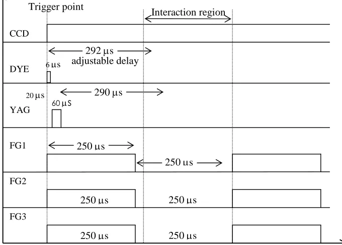
Figure 2: The time chart for image capture. Pin-hole
Nitro -Dye laser
Trig. & Sync. Unit
CCD1
CCD2
CCD3
Nd:YAG laser
Frame grabber PC
Sample
Reference
M1
M2 BS1
BS2
BS3
BS4
CCD
DYE
YAG
FG1
FG2
FG3
292 s
290 s
250 s
60 s 20 s
250 s 6 s
250 s
250 s
250 s
250 s
Interaction region Trigger point
The timing chart (Figure 2) for the sequence of activities between the firing of the lasers and the capture of the images was prepared. It was necessary to delay the illumination of the dye laser by a certain period in order to obtain the illumination of the interaction event. This delay was measured using a high capacitance photodiode connected to an oscilloscope
RESULT AND DISCUSSION
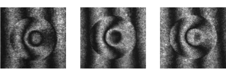
Figure 3: The simultaneously-captured interferograms of laser interaction in air.
Figure 3 shows the three interferograms of an interaction event which have been
separated in phase by 90°. The roundish feature on the interferogram is the interacted
(disturbed) region due to laser interaction. Otherwise, we would have straight and parallel fringes. A reference marker was used to indicate the location of a straight parallel fringe at the center of the interacted region. Laser interaction caused the fringes to deviate from the reference marker due to change in the phase. The size of each interferogram involved in this calculation is 256 x 256 pixels. Initially, Fourier transform filtering was carried out to filter the low frequency background noise and the high frequency digital noise. The measured intensity distribution was Fourier transformed to a linear combination of harmonic spatial functions. In this domain, identification of the signal was made, by removing of the low background frequency and the high noise frequency. Careful identification must be made so as to remove the noise as much as possible and leave the
signal intact.
The simplified intensity equations of the three simultaneously-captured interferograms are
4 , cos 1
, 0
1
x y
I y x
I
4 3 , cos 1
, 0
2
x y
I y x
I (1)
4 5 , cos 1
, 0
3
x y
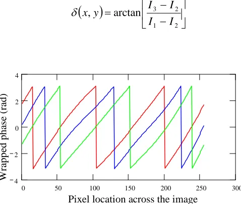
The algorithm chosen for resultant phase (x,y) from the three interferograms is given by Wyant [4].
2 1
2 3 arctan ,
I I
I I y
x
0 50 100 150 200 250 300
4 2 0 2 4
Figure 4 The wrapped phase of the uninterrupted region
0 50 100 150 200 250 300
2 1 0 1 2
Figure 5 The wrapped phase of the interrupted region
Equation (2) gives phase values of the intensity distribution of the fringe pattern which
can be wrapped in the values ranging from – to or from -ð/2 to ð/2. Figure 4 shows the
typical shape of the phase spectrum across the uninterrupted (undisturbed) region of the interferogram after undergoing Fourier-filtering which is often described as a saw-tooth
representation. It shows the phase being wrapped between the values of – to . The
wrapped phase of the interrupted (disturbed) region (through the center of the interferogram) after undergoing Fourier-filtering is shown in Figure 5. This spectrum
was actually wrapped from -ð/2 to ð/2 for greater details. At this stage, the true phase
change of the event cannot be visualized correctly.
W
ra
p
p
ed
p
h
as
e
(r
ad
)
Pixel location across the image Pixel location across the image
W
ra
p
p
ed
p
h
as
e
(r
ad
)
value of the phase angle of a continuous function that extends over a range more than is
recovered [5]. A two-dimensional phase unwrapping processing scheme consists of a
cascade of three operations: differencing, thresholding and integrating [6]. This meant that the neighbouring phase difference must satisfy the required relations over the two-dimensional array, both along the column or lines or any other combinations.
In this work, the unwrapping procedure was also expanded to two and three dimensions. r and s are numbers representing the pixel distribution in the pixel matrix. The mapping of the interferogram follows the algorithm given below [3]
m1,1 = 0 r = 2,3, ………256 s = 2,3,………256
2 1 2 1 2 1 , 1 , 1 1 , 1 1 , 1 , 1 1 , 1 1 , 1 , 1 1 , 1 , 1 s s s s s s s s s s if m if m if m m 2 1 2 1 2 , 1 , , 1 , 1 , , 1 , 1 , , 1 , s r s r s r s r s r s r s r s r s r s r if m if m if m m
r = 1,2……256
s = 1,2,…...256
r,s r,s mr,s
To obtain the values of the phase change due to laser interaction, (x,y), the values
of the phase obtained from the measured disturbed-location should be subtracted from those obtained from the undisturbed location, which was referred to as the reference location
ref
m I I
I I I I I I y x 2 1 2 3 1 2 1 2 3 1 tan tan ,
To perform all the stages of analysis, that is from obtaining its intensity spectrum to Fourier filtering and later the phase analysis, a computer program was written in Mathcad to perform all the necessary tasks in the analysis.
The profile of laser interaction in air was thus produced. After filtering, wrapping (Equation (2) and unwrapping using the algorithm given in Equation (3), the profile of the phase change right across and through the center of the interferogram is given in Figure 6. Compare this with Figure 5 which is its wrapped representation at the same location.
(3)
0 50 100 150 200 250 300 10
5 0 5
Figure 6: The unwrapped phase change through the center of the interferogram
256
1 r
0 50 100 150 200 250 300
10 5 0 5
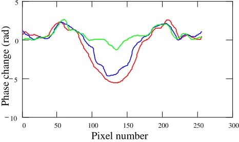
Figure 7: The phase change profile at different locations (slice) of the interferogram
Slices of the profile can be made at any location of the interferogram. These will provide greater detail (quantitatively) of the stages of progress of the changes in the phase which later can be related to other physical parameters of the event. Figure 7 shows the profile of phase change at three locations on the interferogram namely at y = 85, y = 102 and y = 128.
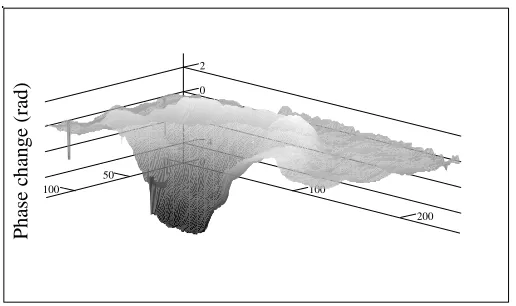
3D images of the events provide a very thorough qualitative observation of the phase change taking place at the region of interaction. Using the computer program, these 3D images can be cut, sliced and viewed from any direction and location requiring detail investigation. The 3D image of the whole interaction event from the captured interferogram is shown in Figure 8. That image can be cut sliced and observed from any angle desired by the observer. Figure 9 shows the image which has been sliced right through the center of the interferogram.
Pixel number
P
h
as
e
ch
an
g
e
(r
ad
)
Pixel number
P
h
as
e
ch
an
g
e
(r
ad
0 100
200 0
100 200
5 0 5
Figure 8: The 3D image of the phase change
0
100
200 0
50 100
4 2 0 2
Figure 9: The 3D image of the cross –section of phase change
CONCLUSION
To eliminate the problem of phase ambiguity in single interferogram phase-mapping, a 3- simultaneously-captured interferograms system was developed. Phase mapping the event in 2D and 3D allows quantitative as well as qualitative analysis to be made. Using the appropriate algorithms in a computer program written in Mathcad, the associated phase change could be successfully extracted and analysed. From the knowledge of the phase change obtained, the associated changes in the other parameters such as the
refractive index, density and pressure could be calculated.
REFERENCES
1. Osten, W. and Juptner, W.. Digital Processing of Fringe Patterns in Optical
Metrology. In: Rastogi, P.K ed. Optical Measurement Techniques and Applications. Boston, London: Artech House Inc. 51-85; 1997.
P
h
as
e
ch
an
g
e
(r
ad
)
P
h
as
e
ch
an
g
e
(r
ad
2. Hariharan, P., Oreb, B.F. and Eiju, T. Digital Phase-Shifting Interferometry: A Simple Error-Compensating Phase Calculation Algorithm. J. Appl. Optics. 1987. 26(13): 2504-2505.
3. Yusof Munajat. High speed Optical Studies for Laser Induced Acoustic Wave and
Phase Measurement Interferometry System. Ph.D. Thesis. Universiti Teknologi
Malaysia: 1997.
4. Wyant, J.C. and K. Creath. Recent Advances in Interferometric Optical Testing.
Laser Focus/Electro Optics. 1985. 118-132.
5. Robinson, D.R. Phase unwrapping method. In: Robinson D.W. and Reid, G.T. eds.
Interferogram Analysis. Bristol: IOP Publishing Ltd. 194-229;1993..
6. Ghiglia, D.C., Mastin, G.A. and Romero, L.A. Cellular automata method for phase