Application of moderate resolution
imaging spectroradiometer snow
cover maps in modeling snowmelt
runoff process in the central Zab
basin, Iran
Himan Shahabi
Saeed Khezri
spectroradiometer snow cover maps in
modeling snowmelt runoff process in the
central Zab basin, Iran
Himan Shahabi,
aSaeed Khezri,
bBaharin Bin Ahmad,
aand
Tajul Ariffin Musa
caUniversiti Teknologi Malaysia, Institute of Geospatial Science & Technology, Skudai 81310, Johor Bahru, Malaysia
bUniversity of Kurdistan, Department of Physical Geography, Faculty of Natural Resources, Iran cUniversiti Teknologi Malaysia, UTM-GNSS and Geodynamics Research Group, Faculty of
Geoinformation and Real Estate, 81310 UTM Skudai, Johor, Malaysia
Abstract.Snow, as one form of precipitation, plays a very significant role in the water cycle and in water resource management. However, the spatial and temporal variations in snow cover com-plicate the monitoring of this role. Field measurements, especially in mountainous areas, are often impossible without the use of new technologies. In this study, moderate resolution imaging spectroradiometer (MODIS) at 500-m resolution has been used to provide a map of snow cover area (SCA) using the normalized difference snow index in the central Zab basin in West Azerbaijan, Iran. Eight-day composite data are used to minimize the effect of cloud cover and maximize the amount of useable SCA images. The importance of snow in this basin was simulated using a snowmelt runoff model (SRM) as one of the major applications of daily MODIS-8 images based on various algorithms. The location of snow gauge stations on digital elevation model (DEM) of central Zab basin extracted from advanced space borne thermal emission and reflection radiometer images by using bilinear interpolation method. The SCA index, along with spectral threshold on bands 2 and 4, provided a stable relationship for extraction of the snow cover map in the study area. The simulated flow in the water year 2010 to 2011 had a coefficient of determination (R2) of 0.8953 and a volume difference (Dv) of 0.1498%, which shows a good correlation between the measured and computed runoff by using the SRM in the central Zab basin. The first results of the modeling process show that MODIS snow covered area product can be used for simulation and measuring value of snowmelt runoff in central Zab basin. The studies found that the SCA results were more reliable in the study area.© The Authors. Published by SPIE under a Creative Commons Attribution 3.0 Unported License. Distribution or reproduction of this work in whole or in part requires full attribution of the origi-nal publication, including its DOI.[DOI:10.1117/1.JRS.8.084699]
Keywords:moderate resolution imaging spectroradiometer; snow cover area; snowmelt runoff model; remote sensing; central Zab basin.
Paper 13232SS received Jul. 13, 2013; revised manuscript received Nov. 5, 2013; accepted for publication Jan. 10, 2014; published online Apr. 2, 2014.
1 Introduction
Iran is a low-water country located in an arid and semiarid region of the Earth. Therefore, snow-fall is considered as the most important factor affecting water supply, especially in the summer, and also snowfall is one of the important factors that controls the hydro-climate of the geographi-cal area. In northwest Iran, precipitation occurs more frequently in the form of snow in the cold seasons, and due to the mountainous characteristics of this area, snow resources persist through-out the year. Consequently, the scientific management of water supplies in the form of snow is necessary to maintain a supply of consumable water.1,2
and especially the spatial and temporal distribution of snowfall and soil moisture, is required for the characterization of runoff.3However, these data are often scattered and of poor quality, but remote sensing has good potential to eliminate these shortcomings.
Snow measurement and assessment in mountainous areas are difficult due to lack of appro-priate access. The diverse features of topography and physiography also complicate the estima-tion of hydrological snow parameters and the inadequate numbers of weather staestima-tions in the highlands point to the necessity of using indirect methods applications, such as the analysis of remote sensing data for measuring snow cover area (SCA).4Satellite images and application of the available algorithms allow extraction of SCA with a reasonable accuracy. The estimation of snow cover surface significantly improves the process of calculation and application of snowmelt models using remote sensing images.5–7
However, these issues have already been partially resolved by the MODIS instrument onboard the environmental remote sensing satellites of the Earth observing systems (EOSs) Terra (EOS-AM1) and Aqua (EOS-PM1), which were launched successfully in 1999 and in 2002, respec-tively.8–10 The MODIS Terra satellite crosses the equator at about 10.30 a.m. (descending orbit) UTC, with a scanning swath of 2330 km (cross-track) by 10 km (along-track at nadir). The MODIS has a total of 36 different wavelength channels suited for a wide range of applications. An algorithm has been developed by Hall et al.8to map snow cover at 500-m spatial resolution using the MODIS observations. The 500-m spatial resolution results from the use of the MODIS bands with demonstrated capability for detecting snow and separating snow from clouds.11 Assessment of the MODIS snow product accuracy and execution of applied research is now pos-sible,12and many scientists are now focusing on the study of snow and ice (e.g., Refs.13–20). These studies have examined the relative accuracy of snow mapping for various snow cover products or the relationship between snow mapping accuracy and spatial resolution, ruggedness, snow depth, or land cover type. The snowmelt runoff model (SRM) has been successfully tested in numerous mountainous basins around the world (e.g., Refs.21–29). The main advantage of temperature index models (i.e., SRM), over other model types, is that they only require air temperature data to obtain estimates of melt.30 The wide availability of these data (mainly in mountainous areas) has led to the popularity of temperature index models, especially in operational stream flow forecasting.31
The purposes of this research are: (a) to investigate the capability of MODIS-8 daily images at 500-m resolution to provide the map of SCA32 and recognize changes in snow cover using the normalized difference snow index (NDSI); (b) to compare snow cover maps extracted from MODIS with the ground-based snow courses at some selected points in the central Zab basin to yield snow water equivalent (SWE); (c) to perform an SCA validation using the MODIS products during the water year 2010 to 2011 for accumulation and ablation periods; and (d) to use the SRM model to model the snowmelt runoff in the study area.
2 Study Area
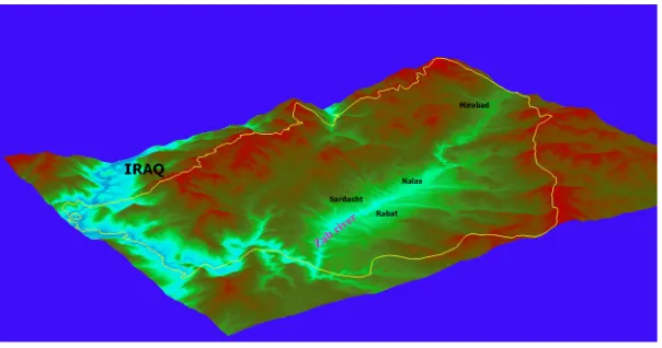
The study area is located in the southwest mountainous area of West Azerbaijan province, Iran, along the Zab river basin in Sardasht, between the latitudes of 36° 8’25”N and 36° 26’27”N and the longitudes of 45° 21’21”E and 45° 40’44”E. The central part of the Zab river basin stretches 30 km from north to south and east to west (Fig.1).
The whole study area is520 km2; 30.45% is located in the west and 69.55% is located east of the main river.33Wherever the size of the catchment of waterways is greater, the rate of flow and volume of alluvial cone material will be higher. In western part of central Zab basin, the rate of flow and volume of runoff is low.
3 Materials and Methods
The application of satellite images to model runoff processes obtained from snowmelt was evalu-ated using the MODIS satellite images obtained on 8 different days that signal quantization is 12-bit radiometric. These satellite images have been used because of their ability to provide high temporal separation with a one day return period as well as the high spatial resolution similar to other satellite images.
The data used in this study include: Topographic maps and field data recorded at the snow gauge stations, including Sardasht, Brisweh, and Mirabad (see Fig.2). The SWE was considered for a fixed water year (2010 to 2011), that starts from January until May. Due to closure during the melting season and the limited time for accessing data from the snow gauge stations, the daily
Fig. 1 Geographical position of central Zab basin.
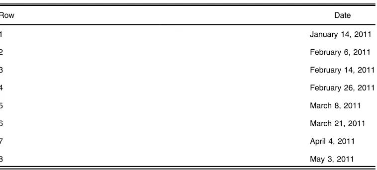
snow cover maps received from MODIS were provided by the Iranian Space Agency with a L1B process level, and are used in deriving the snow depletion curve, which is one of the input param-eters of the SRM (Table1).
The range of the basin and the snow line were determined using base data and topographic maps with a scale of 1:50,000 in digital format. The DEM data were generated from advanced space borne thermal emission and reflection radiometer (ASTER) images provided by the Iranian Space Agency. Images were acquired near the nadir of the 3N band (0.78 to 0.86 μm), and stereo images were acquired for the same area after examining the 3B band (0.78 to 0.86 μm). The ASTER 3N and 3B images were designed for the DEM creation with a Baseline/Height (B/H) from the nadir and aft-telescope of B∕H¼0.6. One hundred tie points were used to form an epipolar image, which had aYparallax¼0.9645.Yparallax comes from a correlation analysis between the 3N band image of the left-hand side and the 3B image of the right-hand side. Therefore, the final DEM is extracted from visible and near-infrared (VNIR¼0.52 to 0.86 μm) in ASTER with a spatial resolution of 15 m. The root of the mean square error (RMSE) of the DEM was 9.80 m. The DEM was generated using the bilinear interpolation method. Figure2 shows the central Zab basin DEM extracted from the ASTER image.
The stages of data preparation were performed using Arc GIS 9.3 software as follows: chang-ing the data format, layer integration, applychang-ing the geometric correction, and extraction of hydro-logic parameters (such as exterminating the basin area range and waterways network). In the processing stage, the MODIS sensor images were extracted during two stages of snow cover: first, in the programming environment of the ERDAS software on the image of the B1 surface, earth operations. The images were referenced with the “Lambert” system and radiometric correction was conducted. The automatic algorithm for snow cover was implemented and the extraction of the SCA was started. In the process of the image processing operation, the following steps were implemented:
In the first stage, reflective criteria were applied if NDSI>0.4. In other words, if the reflec-tance of pixels in band 2 was more than 11% and the reflective value of pixels in band 4 was equal to or more than 10%. Based on above mentioned algorithms, conditional triple tests were conducted to extract the NDSI values.
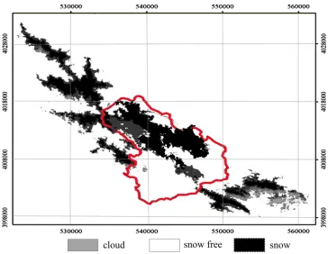
In the second stage, the majority filter was implemented with the aim of reducing the reflec-tance role of a single pixel. This filter is a window of3×3 pixelsand its application classifies the valuable pixels of the specified NDSI as snow cover. Figure3shows the snow, snow free, and cloud covers on February 14, 2011, as 185, 238, and11 km2, respectively.
3.1
Reflective Feature of Snow and the Index of Snow Cover
The reflectance of a snow surface is affected by changes in factors, such as snow grain size, form, water content, surface roughness, snow depth, and impurities as well as the angle of incident
Table 1 The dates of images used for the central Zab basin study.
Row Date
1 January 14, 2011
2 February 6, 2011
3 February 14, 2011
4 February 26, 2011
5 March 8, 2011
6 March 21, 2011
7 April 4, 2011
solar radiation and reflection. Increasing snow age reduces its reflection in the visible spectrum and near-infrared regions, and the main factor in this reduction is an increase in snow grain size due to its melting and refreezing.34The long and short waves received at the snow surface can be an important source of the snowmelt process. The most important feature of snow that causes a difference in the spectral reflection of snow is the difference in the VNIR spectral range.35
A study by Klein et al.36showed that the capability for displaying snow using the MODIS sensor has made significant progress compared to other similar sensors in the unique and high resolution bands. The obtained images have a wide spectral range and the techniques used in the algorithm related to the snow map are based on detection at the local and regional scales.36 Processing is carried out using the images that have characteristics, such as L1B, no clouds, and taken in daylight are selected to extract the snow cover. These pixels must have been recorded during daylight with sufficient light and sky without cloud.37
In this research, the algorithm for the spatial snow cover detection provided by the United States space agency is used so that that the bands 1 to 6 of the MODIS sensor data were studied and analyzed. After applying radiometric and geometric corrections, MODIS/Terra Snow Cover Daily L3 Global 500-m Grid (MOD10A1) is used to snowmelt modeling.
The NDSI is a spectral ratio that uses the spectral difference of the infrared and visible bands in the MODIS sensors to recognize changes in snow cover surface.38The NDSI index takes advantage of the fact that spectral snow reflection has a high reflection in the visible band and low reflection in the spectral range of infrared as a way to discriminate snow from cloud and snow-free areas.39This index, like many spectral ratio methods, reduces atmospheric effects.8
The algorithm of the MODIS snow map from the bands 4 and 6 of this sensor is automatically performed to extract the NDSI and calculated based on [Eq. (1)].40
NDSI¼MODISBand 4−MODISBand 6 MODISBand 4þMODISBand 6
¼green−SWIR
greenþSWIR: (1)
The NDSI index can be used to separate snow and ice from each other and also to separate snow from the clouds at a high atmosphere altitude, like cumulonimbus clouds.41,42This index is
insensitive to the range of lighting conditions and can be adjusted for atmospheric effects. In other words, the NDSI index does not just depend on reflection values in a band but it also depends on the digital number of pixel reflections.43 Pellika and Rees44 proved that pure snow has a high NDSI, but when it is mixed with other substances (such as dust and smoke), the percentage of its purity is reduced. The NDSI index is also used as a separator of cloud-snow from clouds that reflect both VNIR light.
Hall et al.37proved that the algorithm of a snow map is best operated in the condition of full snow cover in areas with thin vegetation, such as grasslands, agricultural fields, and tundra. In these conditions, band 2 of MODIS is mainly processed to detect snow and the NDSI compo-nents of the snow map algorithm effectively filter clouds (with the exception of high altitude clouds). These clouds contain ice pieces and may cause a misclassification of snow cover. According to this criterion, the results of the NDSI index can be accepted if the reflectance of band 2 is more than 11%. The second criterion is introduced as dark targets by Klein et al.36. In this mode, 10% reflection in band 4 is set as the low limit of identification and separation of vegetation from snow. For pixels classified as snow, reflection in band 4 must be equal to or more than 10%. Despite the high value of the NDSI index, in some cases, dark targets prevent correct snow classification. Thus, based on these two criteria, the algorithm for snow cover will consider a pixel as snow if the following conditions are achieved.
This algorithm is used along with two other thresholds:
1. 1-band 2 (0.841 to 0.867μm) has the reflectance of more than 11%.
2. 2-band 4 (0.545 to 0.665μm) has a reflectance equal to or more than 10%. In total, the NDSI index must be estimated as more than 0.4.
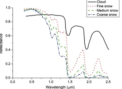
The NDSI index of snow cover is only sensitive to certain types of clouds that have ice particles and some clouds that have reflections similar to that of snow.45Note that cloud typically has high reflectance in the VNIR wavelengths 4 and the value decreases slowly in shortwave infrared wavelengths (SWIR), while snow has high reflectance in visible and NIR and the value decreases significantly in the SWIR (shown in Fig.4).
Li et al.46, to reduce the effects of the snow/cloud misidentification, introduced a normalized difference cloud index (NDCI) model in MODIS data and it is calculated based on [Eq. (2)]:
NDCI¼b1−b6
b1þb6
; (2)
whereb1 andb6are the first and sixth bands of the MODIS data, respectively, whose central wave lengths are 0.66 and 1.64μm, A pixel with an NDCI value greater than 0.1 and less than 0.5 and the apparent reflectance in band 6 >0.4, is identified as a cloudy pixel. The normalized difference vegetation index (NDVI) is calculated as a complement to discriminate between snow-free and snow-covered forests [Eq. (3)]:
NDVI¼b2−b1
b2þb1
; (3)
whereb1andb2are the first and second bands of a MODIS image, respectively. The NDVI and NDSI are used to select snow and nonsnow end members. A pixel known as snow must satisfy three rules simultaneously:47(1) The NDVI values are <−0.4, (2) the NDSI values are>0.8, and (3) the reflectance in MODIS band2 is higher than 0.75. According to these rules, the snow and nonsnow pixels can be extracted.46
3.2
Atmospheric Correction
Reflectance derived from radiance measured by sensors at the top of the atmosphere (TOA) may be increased or decreased when compared to the surface reflectance as a function of the target’s reflectance, its environment, sensor spectral band, viewing and solar geometry, and atmospheric characteristics.48
The snow cover algorithm developed by Hall et al.37uses the TOA reflectance in the NDSI and other thresholds. In Hall et al.’s algorithm, the effects of atmosphere have not been corrected for, which may cause some errors for estimating snow cover in mountainous areas.49Taking into account the computational speed and accurate technique for the atmospheric correction, the surface reflectances are retrieved from the TOA reflectances by using an updated simplified method for the atmospheric correction model in this work.50 If pc is the spectral
surface reflectance of the target, surrounded by a homogeneous environment of spectral reflec-tancepe, the TOA spectral reflectance,p at the satellite level can be expressed as [Eq. (4)]:
pðθs;θv;ΔφÞ ¼tgðθs;θvÞ×
paðθs;θv;ΔφÞ þ ½e−t∕μs þtdðθsÞ
½pce−t∕μvþpetdðθvÞ
1−pes
;
(4)
where μs¼cosðθsÞ ¼cosine of the sun zenith angle, μv ¼cosðθvÞ ¼cosine of the viewing
zenith angle,Δφis the relative azimuth between sun and satellite direction,tgis the total gaseous
transmission (downward and upward path), which takes into account various gaseous absorp-tions,pa is the atmospheric reflectance which is a function of molecule and aerosol optical
properties, illumination angle, viewing angle, and relative azimuth between the sun and the observer,tis the atmospheric optical depth (e−t∕μs ande−t∕μvbeing the direct atmospheric
trans-mittances), tdðθsÞ and tdðθvÞ are the atmospheric diffuse transmittances, pc is the spectral
surface reflectance of the target,pe is the spectral reflectance of an homogeneous environment
surrounding the target, andSis the spherical albedo of the atmosphere. The (1−pes) term takes
into account the multiple scattering between the surface and the atmosphere. For a large target, usually >1 km, the environment effect may be neglected (i.e., pe≈pc) and Eq. (4) can be
simplified to [Eq. (5)]:50
pðθs;θv;ΔφÞ ¼tgðθs;θvÞ
paðθs;θv;ΔφÞ þTðθsÞTðθvÞ
p
1−ps
; (5)
with
TðθÞ ¼e−t∕μþtdðθÞ
whereθ¼θs orθv and μ¼cosðθsÞorcosðθvÞ.
4 Analysis of the Results and Discussion
4.1
Geometric Corrections of Satellite Images
for both positioning and number,52it is possible to rectify images in a very simple manner by ensuring that the resultant RMSE is under a certain threshold.53,54
All rectification methods produce a residual in thexand yaxes between input and output coordinates; for each GCP, RMSE, e.g., the resultant vector from residuals inxandy axes is calculated based [Eq. (6)]:55
RMSE¼pffiffiffiffiffiffiffiffiffiffiffiffiffiffiffiu2þv2; (6)
whereu is residual in thexaxis; vis residual in theyaxis. Total RMSE is then derived as [Eq. (7)]
Total RMSE¼
ffiffiffi
1
n
r Xn i¼1
u2þv2; (7)
wheren is number of GCPs;uis residual in thex axis;vis residual in they axis.
Nearest neighbor resampling method simply associates the nearest original pixel brightness value to the corrected image pixel. For each area and rectification method, total RMSE was calculated, and the dispersion cloud of GCPs residuals was plotted in order to verify the relation between terrain roughness and cloud dimensions.55
The nearest neighbor resampling method with the output pixel dimension of 2 m was per-formed on the SPOT 5 satellite image taken in 2008. The three-dimensional image of the central Zab Basin, extracted using the SPOT 5 satellite, is shown in Fig.5.
Figure6shows an accuracy test of the process of geometric correction using the layer of basin waterways before (A) and after (B) the process of geometric correction.
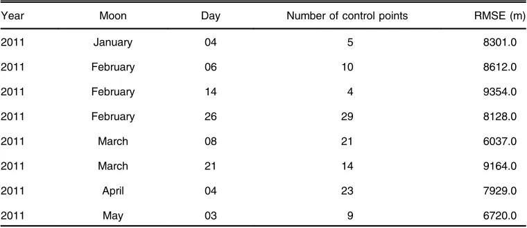
The RMSE produced in the earth process of referencing MODIS satellite images is given in Table2.
4.2
Reflectance of Elements of Earth and Snow in the MODIS Satellite Images
Snow monitoring due to spatial and temporal snow variables depends on the remelting and reraining conditions. In addition, due to the lack of snow telemetry, the phenomenon mentioned in the result of map preparation, geometric accuracy is not possible when studying the accuracy of digital interpretation.
4.3
Providing the Images of Snow-Covered Area
After calculating NDSI and NDVI, the snow cover is determined in pixels according to these two values and other distinct criteria. Note that the reflectances used are the atmospheric corrected reflectances. To prevent errors in pixels containing very dark targets, such as black spruce forests,
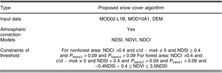
the threshold values of the surface reflectances in MODIS bands 2 (0.841 to 0.876μm) and 4 (0.545 to 0.565 μm) are adjusted to >9%. The NDSI was applied as an equation on the image so that the numbers higher than and equal to 0.4 were isolated as a conditional snow pixel and reflectance in MODIS bands 2 and 4 are >9%. The currently proposed snow cover algorithm for MODIS data is shown in Table3.
As depicted in Fig. 7 in red, the basin surface is considered as snow using this index. Therefore, to separate water from snow and also to separate dark and shadowy areas from snow, the reflections of band 4 were used for dark targets and band 2 for water.56
According to operation in the pixel value or by recoding the reflectance of band 2 higher than 11% and the reflectance of band 4 that was equal or>10%, these values were multiplied in the NDSI image to obtain the final image of the surface snow cover (see Fig.8).
Comparing the real images of MODIS and the image of snow separated by the snow normalized index gave the snow difference. This index separates the snow surface well (Fig. 9). In Iran, mapping of the snow surface is not conducted so that we cannot estimate the accuracy of this index; however, according to a study conducted in the Rio Grande watershed on MODIS snow cover during the years of 2000 to 2001, assessment of the quality of MODIS snow cover maps is accomplished through comparisons of MODIS snow maps with those pro-duced by NOHRSC as well as through comparisons with in situ observations of snow depth calculated from automated measurements of SWE. As the entire snow season is being considered in this study, comparisons of MODIS snow maps were created from higher resolution sensors,
Fig. 6 Accuracy test of the process of geometric correction using the layer of basin waterways before (a) and after (b) the process of geometric correction.
Table 2 The root mean square error (RMSE) produced in the earth process of referencing moderate resolution imaging spectroradiometer (MODIS) satellite images.
Year Moon Day Number of control points RMSE (m)
2011 January 04 5 8301.0
2011 February 06 10 8612.0
2011 February 14 4 9354.0
2011 February 26 29 8128.0
2011 March 08 21 6037.0
2011 March 21 14 9164.0
2011 April 04 23 7929.0
such as Landsat ETM+ or ASTER. These comparisons are, however, being conducted as part of ongoing MODIS validation efforts.13
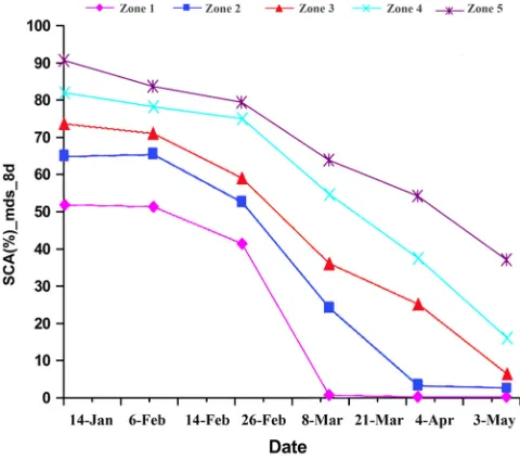
In this study, runoff from snowmelt was modeled by dividing the central Zab basin into 5 elevation zones with around 200-m classes of elevation surfaces in the Arc GIS 9.3, and the snow-covered surface was obtained in each of these separated zones. The amount of SCA in the central Zab basin, using NDSI extracted from the MODIS satellite images, is given in Table4.
The snow depletion curves belonging to each elevation class obtained from the MODIS snow products for central Zab basin are shown in Fig.10.
4.4
Interpolation of Snow-Covered Surface
The covered surface was then interpolated for days without satellite images. The snow-covered surface in the central Zab basin was calculated through the interpolation of the time series of MODIS images based on the algorithm provided by Malcher and Rott.57The satellite carrier MODIS sensor takes images from the surface of earth daily but due to the cost of satellite
Table 3 The proposed snow cover algorithm for MODIS data.
Type Proposed snow cover algorithm
Input data MOD02-L1B, MOD10A1, DEM
Atmospheric correction
Yes
Models NDSI, NDVI, NDCI
Constraints of threshold
For nonforest area: NDCI>0.4andcldmsk≠0and NDSI≥0.4 andPband2>0.09andPband4>0.09For forest area: NDCI>0.4and
cldmsk≠0and NDSI <0.4andPband2>0.09andPband1>0.09and −0.4NDSIþ0.4≤NDVI≤3.5NDSI
Pis surface true reflectance.
imaging and time-consuming nature of the process and daily extraction of snow-covered surfaces in watersheds, the possibility of the daily use of satellite images was virtually ruled out. The complex nature of the snow and its location and time variation meant that the selection of dates of the satellite images was very important and could affect the accuracy of determining the snow-covered surface. Temperature was an additional factor of vital importance, with regard to the process of snow melting in the melting season, as pointed out earlier. The temperature factor has a greater effect than other phenomena, such as rainfall on the snow ridge or the quantities of radiation, in the process of melting snow on snow ridge. Extrapolation of the snow-covered surface is determined based on the temperature of the snowfall in each of the height zones. According to the Malcher algorithm, the melting factor is a function of critical temperature and a degree–day factor and according to Eq. (8), this can be expressed as58
ΔMðt1; t2Þ ¼
Xt2
t2
ðaTÞ; (8)
whereΔMis cumulative snowmelt depth,ais factor degree-day, andTis critical temperature. The snow-covered surface is determined according to the critical temperature based on Eq. (9):59
SðtnÞ ¼Sðtn−1Þ−
Sðt1Þ−Sðt2Þ ΔMðt1; taÞ þΔMðtb; t2Þ
·ΔMðtx−1; txÞ; (9)
where,Sis the area covered by snow in dayn,ΔMis the rate of melt,t1is starting day of melting, t2is final melting day,ta–bis time interval without melting, andtxis the time interval with melting.
Fig. 8 Reflection band 2 (a) and band 4 (b) reflectance criteria used for snow separation.
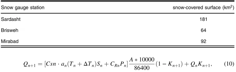
Finally, taking all these factors into account, the snow-covered surface for three snow gauge stations including Sardasht, Brisweh, and Mirabad are obtained with interpolation of the extracted snow-covered surface derived from the MODIS satellite images (Table5).
4.5
Simulation of Snowmelt Runoff
In this research, the snowmelt runoff in the central Zab basin was modeled using the SRM model that provides the snow-covered surface through satellite images and enters it into the model as one of the basic variables. If rain falls on this snow cover, it is assumed that the same amount of water is released from the snowpack so that rain from the entire area is added to snowmelt. The melting effect of rain is neglected because the additional heat supplied by the liquid precipitation is considered to be small. A few models in hydrology also use remote sensing data as input data. The SRM is one of the models that uses remote sensing data directly from hydrological models.60 The model was proposed for the first time by Martinec and Rango60for the proper manage-ment of water resources in the mountainous areas of the Alps, and its Windows version was upgraded in 2003. The main equation of the model, which allows the transformation of water produced from snowmelt and rainfall into the daily discharge, is based on a simple degree-day method.59
In the SRM model, discharge from rainfall and snow melting is calculated on a daily basis. The basic equation of the model is as follows Eq. (10):
Table 4 Amount of snow cover area in the central Zab basin using the normalized difference snow index (NDSI) extracted from MODIS satellite images.
Zone Area (km2) Mean elevation (m)
Snow covered area (%)
Date of measurement (2011)
04-01 06-02 14-02 26-02 08-03 21-03 05-04 03-05 Mean
1 135 950 4 9 14 22 16 10 5 2 10
2 124 1600 5 11 18 28 21 19 13 5 15
3 99 1900 7 15 21 34 26 17 12 7 17
4 83 2100 14 18 25 40 32 24 20 9 22
5 79 2500 12 18 37 41 34 31 19 6 24
Qnþ1¼ ½Csn·anðTnþΔTnÞSnþCRnPn
A10000
86400 ð1−Knþ1Þ þQnKnþ1; (10)
where Qis the average daily discharge (m3·S−1),C is the runoff coefficient expressing the losses as a ratio of runoff to precipitation, with Cs referring to snowmelt CR to rain; a is
the degree-day factor (cm· °C·d−1), which indicates the snowmelt depth resulting from one degree-day; T is the number of degree-days (°C·d); ΔT is the adjustment by temperature lapse rate when extrapolating the temperature from the station to the average elevation of the basin or zone (°C·d);Sis the ratio of the SCA to the total area;Pis the precipitation con-tributing to runoff (cm), which is determined by the preselected threshold temperature;Ais the area of the basin or zone (km2);kis the recession coefficient indicating the decline of discharge in a period without snowmelt or rainfall;k¼Qmþ1∕Qm(mandmþ1are the sequence of days
during a true recession flow period); andnis the sequence of days during the discharge com-putation period. The conversion fromcm·km2 ·d−1tom3 ·s−1(conversion from runoff depth to discharge) is 10,000/86,400.61
The degree-days are used to determine the melt rate of the snowpack in the area of the basin covered by snow as observed from satellites. The degree-day factor is not a constant, and changes in response to changing snow properties and atmospheric conditions. Martinec59 devel-oped the following relationship for the computation of the degree-day factor (a), which takes into account the positive correlation between snow density and the degree–day factor Eq. (11):
a¼ps pw
; (11)
whereρs(g cm−3) andρw(1 g m−3) are the densities of snow and water. Daily SWE and snow depth data, obtained from snow gauge stations, are used to estimate the density of the snowpack. The density of the snowpack is calculated using the following Eq. (12):62
ps¼ ðSWEpwÞ∕ds; (12)
wheredsis the depth of the snowpack (cm). Since there is more than one snow gauge station in
each of the test basins, basin-wide average values (time-series) are obtained and applied to each elevation zone.
Along with the topographic, meteorological, and hydrologic parameters, snow melt simu-lation requires 11 parameters and variables, as follows: recession coefficient, time lag, critical temperature, runoff coefficient for snow, runoff coefficient for rain, degree-day factor, rainfall contributing area, reference elevation, temperature lapse rate, precipitation lapse rate, and initial discharge; these were all considered as input parameters to the SRM model. The parameter val-ues used for the central Zab basin are given in Table6.
Determination of the SRM model parameters for the central Zab basin is related to the basin size to some extent. Usually, it seems more complex in a large basin covering a variety of cli-matic zones than in a small basin with relatively simple features. Because the quality of the input data is directly related to the model accuracy and efficiency, the calculation and determination of variables and parameters is most important to SRM. Hence, according to previous studies, the SRM research worldwide has been mainly concentrated on the acquisition of variables, opti-mization of parameters, and proper analyses of the hydrological and physical characteristics of a basin. All the variables and parameters have to be specified for model input on a daily step. The SRM calculates the daily average stream flow on the (nþ1)’th day by the addition of snowmelt and precipitation contributing to runoff and discharge on the preceding day.
Table 5 The snow-covered surface for three snow gauge stations obtained from MODIS satellite images.
Snow gauge station snow-covered surface (km2)
Sardasht 181
Brisweh 64
4.5.1
Validation of the SRM model
Generally, the results of the model are verified by comparison between the computed and mea-sured discharge. The computed and meamea-sured discharges were plotted and the graphs matched well with each other. Apart from the visual observation, the model accuracy can also be checked by statistical parameters. The SRM model used two other accuracy criteria based on the statistical coefficients: one is the coefficient of determination (R2) and the second is the volume difference (Dv). The equations for R2 and Dv are as follows Eq. (13):48
R2¼1−
Pn
i¼1ðQi−Qi0Þ
2
Pn
i¼1ðQi−Q¯Þ2
; (13)
whereQi,Qi0 are the observed and simulated discharge, respectively, while Q
−
is the average observed discharge. The deviation of runoff volumes,Dv, is computed as follows Eq. (14):
Dv½% ¼
VR−VR0
VR
100; (14)
whereVR is the simulated volume, andVR0 is the observed volume.
By calculating and entering these input variables and parameters, a snowmelt runoff hydro-logical model (SRM) was generated.63The comparison between the observed discharge and that calculated by the SRM model is shown in Fig.11.
The statistical criterion for evaluation of the efficiency of fit between the observed and cal-culated values was applied. The coefficient of determination (R2) for simulation was 0.8953, which shows a good correlation between the observed and calculated values. Another index was theDv ratio. The Dv value for the simulation run was 0.1498%. The average measured
runoff and average computed runoff were obtained as 23.156 and23.161 m3∕s, respectively (see Fig. 11). The error rate for snowmelt runoff modeling using the mean comparison test (t-test) was calculated as 0.384. According to the values obtained from thet-test statistical pro-file, the measured flow rate showed no significant difference at the 93% confidence interval. These results suggest that the SRM can successfully simulate both diurnal water discharge and SWEs in the mountainous study area.
Table 6 Parameter values used in the snowmelt runoff model for snow melt simulation in the central Zab basin.
Parameter Range
Recession coefficient (k) x¼1.121,y¼0.018
Time lag 18 h
Critical temperature 0.65°C to 4°C
Runoff coefficient for snow 0.5 to 0.83
Runoff coefficient for rain 0.5 to 0.96
Degree-day factor 0.4 to 0.65
Rainfall contributing area 0 (Feb to May)
Reference elevation 980 m
Temperature lapse rate 0.5°C∕100m
Precipitation lapse rate 6.5 mm
5 Conclusions
The use of satellite images to monitor natural phenomena such as snow cover is recommended due to considerable reductions in costs and time. Continuous monitoring of snow requires sen-sors with a short repeat period and with precise ability for ground separation and good color separation. The results of the present study show that the MODIS-8 daily images are appropriate for extract snow cover and use it for snowmelt estimation. The reason for using 8-day snow cover maps instead of daily ones was the fact that there was no ground truth data that might have increased the accuracy of the daily image. However, 8-day snow cover maps have the possibility that cloud that contaminated grid cells might have been determined as cloud-free and incorrectly classified. The forecasting studies show that the use of the MODIS snow maps appear to be expedient for prediction of the magnitude and timing of snowmelt runoff that contributes large volumes of flows to reservoirs.
The output hydrograph indicates that the major water resources of the central Zab basin are supplied from snowfall. The delayed effect of snow on the basin flow is also seen in the output hydrographs that show the necessity of managing water resources in this basin to reduce the damage caused by snowmelt flooding in early melting season and during spring with rain fall in the warm days of this season where the temperature of raindrops is high. Thus, quick and accurate information about the snow coverage is very important for operational forecasting and simulating water resource applications. For simulation of the runoff resulting from snowmelt in the snow gauge stations that are lacking in information about the snow coverage, the SRM model provides SCAs in the regions by providing these data from satellite images. Considering that snow gauge data collection is not done in most basins in Iran, this method is considered as an excellent alternative. The efficiency of the model’s applications in several mountainous sub-catchments of the basin showed that the model performed accurately in snowmelt estimation of most basins.
Acknowledgments
First and foremost, the first author would like to thank the Universiti Teknologi Malaysia (UTM) and University of Kurdistan, Iran, for providing the facilities for this investigation. The author also would like to thank the two anonymous reviewers for the constructive comments which
significantly improved the quality of this paper. The authors are also grateful to the Editor-in-Chief Dr. Wei Gao and Associate Editor Dr. Huadong Guo for their helpful comments and suggestions that enabled us to improve the paper.
References
1. P. Romanov, G. Gutman, and I. Csiszar,“Automated monitoring of snow cover over North America with multispectral satellite data,”J. Appl. Meteorol. 39(11), 1866–1880 (2000), http://dx.doi.org/10.1175/1520-0450(2000)039<1866:AMOSCO>2.0.CO;2.
2. H. Shahabi and B. Ahmad,“Application of MODIS image satellite and GIS technique in assessment of avalanche fall in roads,” Proc. World Acad. Sci., Eng. Technol. 57(10), 713–717 (2011).
3. H. Shahabi, A. Piroti, and M. Ahadnezhad, “Mountainous snow cover monitoring and snowmelt runoff discharge modeling in the Langtang Khola catchment,” in 6th Int. Symp. Digital Earth (ISDE6), Beijing, China (2009).
4. G. Kite and A. Pietroniro, “Remote sensing applications in hydrological modelling,”
Hydrol. Sci. J.41(4), 563–591 (1996), http://dx.doi.org/10.1080/02626669609491526. 5. G. Kite,“A watershed model using satellite data applied to a mountain basin in Canada,”J.
Hydrol.128, 157–169 (1991),http://dx.doi.org/10.1016/0022-1694(91)90136-6.
6. P. Singh and S. Jain,“Modelling of streamflow and its components for a large Himalayan basin with predominant snowmelt yields,”Hydrol. Sci. J.48(2), 257–276 (2003),http://dx .doi.org/10.1623/hysj.48.2.257.44693.
7. R. Gupta, U. Haritashya, and P. Singh, “Mapping dry/wet snow cover in the Indian Himalayas using IRS multispectral imagery,” Remote Sens. Environ. 97(4), 458–469 (2005),http://dx.doi.org/10.1016/j.rse.2005.05.010.
8. D. K. Hall et al.,“MODIS snow-cover products,”Remote Sens. Environ.83(1–2), 181–194 (2002),http://dx.doi.org/10.1016/S0034-4257(02)00095-0.
9. D. K. Hall and G. A. Riggs,“Accuracy assessment of the MODIS snow products,”Hydrol. Processes21(12), 1534–1547 (2007), http://dx.doi.org/10.1002/(ISSN)1099-1085. 10. X. Wang et al.,“Comparison and validation of MODIS standard and new combination of
Terra and Aqua snow cover products in northern Xinjiang, China,”Hydrol. Processes23(3), 419–429 (2009), http://dx.doi.org/10.1002/hyp.v23:3.
11. A. E. Tekeli et al.,“Using MODIS snow cover maps in modeling snowmelt runoff process in the eastern part of Turkey,”Remote Sens. Environ.97(2), 216–230 (2005),http://dx.doi .org/10.1016/j.rse.2005.03.013.
12. X. Yap and M. Hashim,“A robust calibration approach for PM 10 prediction from MODIS aerosol optical depth,”Atmos. Chem. Phys.13(6), 3517–3526 (2013),http://dx.doi.org/10 .5194/acp-13-3517-2013.
13. A. G. Klein and A. C. Barnett,“Validation of daily MODIS snow cover maps of the Upper Rio Grande River Basin for the 2000–2001 snow year,”Remote Sens. Environ.86(2), 162– 176 (2003),http://dx.doi.org/10.1016/S0034-4257(03)00097-X.
14. E. P. Maurer et al., “Evaluation of the snow-covered area data product from MODIS,”
Hydrol. Processes17(1), 59–71 (2003),http://dx.doi.org/10.1002/(ISSN)1099-1085. 15. D. Vikhamar and R. Solberg,“Snow-cover mapping in forests by constrained linear spectral
unmixing of MODIS data,” Remote Sens. Environ.88(3), 309–323 (2003), http://dx.doi .org/10.1016/j.rse.2003.06.004.
16. M. Rodell and P. Houser, “Updating a land surface model with MODIS-derived snow cover,” J. Hydrometeorol. 5(3), 1064–1075 (2004), http://dx.doi.org/10.1175/ JHM-395.1.
17. S. J. Déry et al.,“An approach to using snow areal depletion curves inferred from MODIS and its application to land surface modelling in Alaska,”Hydrol. Processes19(4), 2755– 2774 (2005),http://dx.doi.org/10.1002/(ISSN)1099-1085.
18. S. Lee, A. G. Klein, and T. M. Over,“A comparison of MODIS and NOHRSC snow-cover products for simulating streamflow using the Snowmelt Runoff Model,”Hydrol. Processes
19. X. Zhou, H. Xie, and J. M. Hendrickx, “Statistical evaluation of remotely sensed snow-cover products with constraints from streamflow and SNOTEL measurements,”
Remote Sens. Environ. 94(12), 214–231 (2005), http://dx.doi.org/10.1016/j.rse.2004.10 .007.
20. A. Simic et al., “Validation of VEGETATION, MODIS, and GOES+ SSM/I snow-cover products over Canada based on surface snow depth observations,” Hydrol. Processes
18(6), 1089–1104 (2004),http://dx.doi.org/10.1002/(ISSN)1099-1085.
21. R. Brown and C. Derksen,“Is Eurasian October snow cover extent increasing?,”Environ. Res. Lett.8(5), 024006 (2013),http://dx.doi.org/10.1088/1748-9326/8/2/024006.
22. D. K. Hall and J. Martinec,Remote Sensing of Ice and Snow, Chapman and Hall, London (1985).
23. B. Dey, V. Sharma, and A. Rango,“A test of snowmelt-runoff model for a major river basin in western Himalayas,”Nordic Hydrol.20(3), 167–178 (1989),http://dx.doi.org10.2166/nh .1989.013.
24. A. Rango and V. Katwijk,“Development and testing of a snowmelt-runoff forecasting tech-nique,”JAWRA J. Am. Water Res. Assoc.26(1), 135–144 (1990),http://dx.doi.org/10.1111/ jawr.1990.26.issue-1.
25. J. Martinec et al.,Snowmelt Runoff Model (SRM) User’s Manual, Geographisches Institut der Universität, Maryland, USA (1994).
26. K. M. Mitchell and D. R. DeWalle,“Application of the snowmelt runoff model using multi-ple-parameter landscape zones on the Towanda Creek basin, Pennsylvania,”JAWRA J. Am. Water Res. Assoc.34(2), 335–346 (1998),http://dx.doi.org/10.1111/jawr.1998.34.issue-2. 27. R. Ferguson,“Snowmelt runoff models,”Prog. Phys. Geogr.23(2), 205–227 (1999),http://
dx.doi.org/10.1177/030913339902300203.
28. J. Wang and W. Li,“Establishing snowmelt runoff simulating model using remote sensing data and GIS in the west of China,”Int. J. Remote Sens.22(17), 3267–3274 (2001),http://dx .doi.org/10.1080/01431160010030082.
29. E. Gómez-Landesa and A. Rango,“Operational snowmelt runoff forecasting in the Spanish Pyrenees using the snowmelt runoff model,”Hydrol. Processes16(8), 1583–1591 (2002), http://dx.doi.org/10.1002/(ISSN)1099-1085.
30. H. Ma and G. Cheng,“A test of Snowmelt Runoff Model (SRM) for the Gongnaisi River basin in the western Tianshan Mountains, China,” Chin. Sci. Bull. 48(20), 2253–2259 (2003),http://dx.doi.10.1007/BF03182862
31. T. Nagler et al.,“Assimilation of meteorological and remote sensing data for snowmelt run-off forecasting,” Remote Sens. Environ. 112(4), 1408–1420 (2008), http://dx.doi.org/10 .1016/j.rse.2007.07.006.
32. P. Sirguey, R. Mathieu, and Y. Arnaud,“Subpixel monitoring of the seasonal snow cover with MODIS at 250 m spatial resolution in the Southern Alps of New Zealand: method-ology and accuracy assessment,”Remote Sens. Environ.113(1), 160–181 (2009),http://dx .doi.org/10.1016/j.rse.2008.09.008.
33. H. Shahabi, B. Ahmad, and S. Khezri,“Evaluation and comparison of bivariate and multi-variate statistical methods for landslide susceptibility mapping (case study: Zab basin),”
Arab. J. Geosci.6(10), 1–23 (2012),http://dx.doi.org/10.1007/s12517-012-0650-2. 34. V. Salomonson and I. Appel,“Estimating fractional snow cover from MODIS using the
normalized difference snow index,” Remote Sens. Environ. 89(3), 351–360 (2004), http://dx.doi.org/10.1016/j.rse.2003.10.016.
35. S. Wuttke, G. Seckmeyer, and G. König-Langlo,“Measurements of spectral snow albedo at Neumayer, Antarctica,” Ann. Geophys. 24(2), 7–21 (2006), http://dx.doi.org/10.5194/ angeo-24-7-2006.
36. A. G. Klein, D. K. Hall, and G. A. Riggs,“Global snow cover monitoring using MODIS,”
Inform. Sustainability, 363–366 (1998).
37. D. K. Hall et al.,“Algorithm theoretical basis document (ATBD) for the MODIS snow and sea ice-mapping algorithms,”Hydrol. Sci. Branch NASA(2001)http://modis-snow-ice.gsfc .nasa.gov/?c=sug_main.
39. J. Dozier,“Spectral signature of alpine snow cover from the Landsat Thematic Mapper,”
Remote Sens. Environ.28, 9–22 (1989),http://dx.doi.org/10.1016/0034-4257(89)90101-6. 40. D. K. Hall, G. A. Riggs, and V. V. Salomonson,“Development of methods for mapping global snow cover using moderate resolution imaging spectroradiometer data,” Remote Sens. Environ.54(2), 127–140 (1995),http://dx.doi.org/10.1016/0034-4257(95)00137-P. 41. A. W. Nolin and S. Liang,“Progress in bidirectional reflectance modeling and applications
for surface particulate media: snow and soils,”Remote Sens. Rev.18(2–4), 307–342 (2000), http://dx.doi.org/10.1080/02757250009532394.
42. L. Geosystems,“ERDAS imagine,”Atlanta, Georgia (2004).
43. P. Cobb,“Assessing the performance of several Modis level-2 cloud and aerosol products against a surface based polarization cloud lidar at Fairbanks, AK,” Master’s Thesis, University of Alaska, Fairbanks (2008).
44. P. Pellika and W. G. Rees, Remote Sensing of Glaciers: Techniques for Topographic, Spatial and Thematic Mapping of Glaciers, Taylor & Francis, London (2009).
45. D. R. Archer et al.,“The potential of satellite remote sensing of snow over Great Britain in relation to cloud cover,”Nordic Hydrol.25(1–2), 39–51 (1994).
46. W. Li et al.,“Cloud detection in MODIS data based on spectrum analysis,”Geomat. Inf. Sci. Wuhan Univ.30(5), 435–438 (2005).
47. B. H. Tang et al.,“Determination of snow cover from MODIS data for the Tibetan Plateau region,”Int. J. Appl. Earth Observ. Geoinf.21, 356–365 (2013),http://dx.doi.org/10.1016/j .jag.2012.07.014.
48. C. M. Shreve et al.,“Indices for estimating fractional snow cover in the western Tibetan Plateau,” J. Glaciol. 55(192), 737–745 (2009), http://dx.doi.org/10.3189/ 002214309789470996.
49. J. Zhu, J. Shi, and Y. Wang,“Subpixel snow mapping of the Qinghai–Tibet Plateau using MODIS data,”Int. J. Appl. Earth Observ. Geoinf.18, 251–262 (2012),http://dx.doi.org/10 .1016/j.jag.2012.02.001.
50. M. S. Shad, M. H. Roshan, and A. Ildoromi,“Integration of the MODIS snow cover pro-duced into snowmelt runoff modeling,”J. Indian Soc. Remote Sens., 1–11 (2013),http://dx .doi.org/10.1007/s12524-013-0279-y.
51. P. Sirguey,“Simple correction of multiple reflection effects in rugged terrain,”Int. J. Remote Sens.30(4), 1075–1081 (2009), http://dx.doi.org/10.1080/01431160802348101.
52. H. Rahman and G. Dedieu,“SMAC: a simplified method for the atmospheric correction of satellite measurements in the solar spectrum,”Remote Sens.15(1), 123–143 (1994),http:// dx.doi.org/10.1080/01431169408954055.
53. K. E. Rittger, “Spatial estimates of snow water equivalent in the Sierra Nevada,” PhD Dissertation, University of California, Santa Barbara (2012).
54. P. J. Gibson et al., Introductory Remote Sensing: Digital Image Processing and Applications, Vol. 11, Routledge, London (2000).
55. D. Rocchini and A. Di Rita,“Relief effects on aerial photos geometric correction,”Appl. Geogr.25(2), 159–168 (2005),http://dx.doi.org/10.1016/j.apgeog.2005.03.002.
56. P. Zhang et al.,“Application of SRM to flood forecast and forewarning of Manasi River basin in spring,”Remote Sens. Technol. Appl.24, 456–461 (2009).
57. P. Malcher and H. Rott,“Methods for snow area retrievals in alpine regions by means of optical satellite sensors,”EnviSnow EVG1-CT-2001-00052 (2004).
58. P. Malcher et al., inProcess. Data Assimilation Scheme for Satellite Snow Cover Products
in the Hydrological Modeled: Deliverable(2004).
59. J. Martinec, “Snowmelt-runoff model for stream flow forecasts,” Nordic Hydrol. 6(3), 145–154 (1975), http://dx.doi.org/10.2166/nh.1975.010.
60. J. Martinec and A. Rango,“Parameter values for snowmelt runoff modelling,”J. Hydrol.
84(3–4), 197–219 (1986),http://dx.doi.org/10.1016/0022-1694(86)90123-X.
61. M. Georgievsky, “Application of the Snowmelt Runoff model in the Kuban River basin using MODIS satellite images,” Environ. Res. Lett. 4(4), 045017 (2009), http://dx.doi .org/10.1088/1748-9326/4/4/045017.
63. S. Abudu et al.,“Application of snowmelt runoff model (SRM) in mountainous watersheds: a review,” Water Sci. Eng. 5(2), 123–136 (2012), http://dx.doi.org/10.3882/j.issn.1674-2370.2012.02.001.
Himan Shahabiis currently a PhD student of remote sensing (natural hazards) at the Universiti Teknologi Malaysia (UTM). He received his MSc in geomorphology in 2009 at the University of Tabriz, Iran. He finished his BS in physical geography (geomorphology) in 2007 at the University of Tehran, Iran. His interest research fields are environmental assessment and mod-eling, landslide susceptibility mapping, natural hazards and disaster management in urban planning.
Saeed Khezriis assistant professor in geomorphology in the Department of Physical Geography at the University of Kurdistan, Iran. He received a PhD degree in geomorphology in 2006 and a master’s degree in hydroclimatology in 1997 at the University of Tabriz.
Baharin Bin Ahmadis associate professor in remote sensing, faculty of Geoinformation and Real Estate in Universiti Teknologi Malaysia (UTM). He finished his PhD degree in geography in New South Wales, Australia. He received a master’s degree in surveying and mapping in Curtin, Australia.