Changes in Beta Decay Rates Due to the Influence of the Sun.

BALCI, SUMEYRA. Investigation of Possible Changes in Beta Decay Rates Due to the Influence of the Sun. (Under the direction of Christopher Gould.)

There is a growing interest in searching for seasonal effects on nuclear decay rates.

Based on this interest, a data set taken at the Nuclear Reactor Program in Burlington

Laboratory at North Carolina State University has been studied. A Radium-226 source was

used to calibrate a gamma ray spectrometer system on a weekly basis over a 17-year period.

The data have been analyzed by subtracting yearly means and by performing a regression

analysis with a SAS program. We find a seasonal variation at the 5𝜎 level, which is however

not in phase with the earth-sun distance. A natural explanation, that the variation is due to

changes in Radon in the room, is considered, and found to be not consistent with the size of

© Copyright 2013 by Sumeyra Balci

Investigation of Possible Changes in Beta Decay Rates Due to the Influence of the Sun

by Sumeyra Balci

A thesis submitted to the Graduate Faculty of North Carolina State University

in partial fulfillment of the requirements for the Degree of

Master of Science

Physics

Raleigh, North Carolina

2013

APPROVED BY:

Daniel Stancil John Blondin

Christopher Gould

DEDICATION

BIOGRAPHY

The author was born and raised in Konya, Turkey. She completed her Bachelor’s of Science

in Physics at Fatih University in Istanbul, Turkey with honors with a degree in June 2009.

Soon after, she went to the U.S. to pursue a graduate degree in Physics at North Carolina

State University, in Raleigh, NC, USA. During that time, she discovered an interest in

Nuclear Physics, started her research and wrote a Masters thesis on it.

ACKNOWLEDGEMENTS

First and foremost I would like to thank to my advisor Prof. Christopher Gould for all

his contributions in the form of corrections, suggestions and valuable guidance throughout

my research. I am thankful to my committee members: Prof. John Blondin and Prof. Daniel

Stancil for their interest in my work.

I would like to thank Prof. Dave Dickey and Joy Smith for their help during SAS

analysis. Also special thanks to laboratory manager Scott Lassell for his patience and support

and Gerry Wicks for carrying out a direct radon measurement.

Last but not least, I would like to express my appreciation to my lovely family for

their encouragement for my life and my friends, especially Seyma Nur Ozcan, for their love

TABLE OF CONTENTS

LIST OF TABLES

vii

LIST OF FIGURES

viii

Chapter 1. Introduction

1

1.1 Introduction to Radioactivity

1

1.2 Radioactive Decay Law

1

1.3 Types of Decay

3

1.3.1 Alpha Decay

4

1.3.2 Beta Decay

5

1.3.3 Gamma Decay

7

1.4 Literature Review

8

Chapter 2. Nuclear Reactor Program

10

2.1 PULSTAR Reactor and Neutron Activation Analysis Program

10

2.2 Detectors and Electronics

13

2.3 Radium Beta Decay Source

23

2.4 Analysis the Spectra

25

Chapter 4. Possible Explanations for the Seasonal Variation

37

4.1 Sun-Earth Distance

37

4.2 Radon Background in the Laboratory

39

Chapter 5. Summary and Future Work

44

REFERENCES

46

LIST OF TABLES

Table 2.1 Nuclides, Half-lives, Decay Modes, and Daughter Nuclides…………... 25  

Table 3.1 SAS Output: Parameter Estimates……… 33  

LIST OF FIGURES

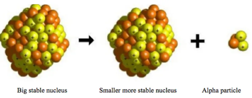
Figure 1.1 Alpha decay of a nucleus. An unstable nucleus becomes more stable by

emitting the alpha particle………

4  

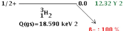
Figure 1.2 The decay level schematic of Tritium (or 3H)……….. 5  

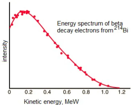
Figure 1.3 Energy spectrum of beta decay electrons from Bismuth-214. The x-axis

represents the kinetic energy in MeV and the y-axis represents

intensity. The figure shows that energies of electrons have a continuous

spectrum………

7  

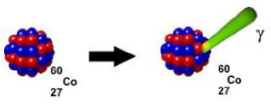
Figure 1.4 Gamma decay of Co-60. The atomic number and the mass number do

not change in this decay mode………..

8  

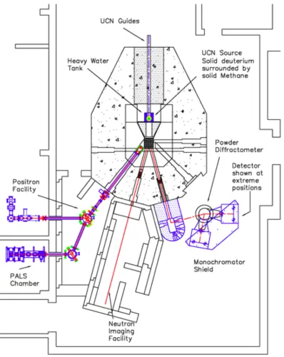
Figure 2.1 Schematic of PULSTAR Reactor. There are 4 types of facilities

working currently. Neutron Powder Diffraction Facility (NPDF),

Neutron Imaging Facility (NIF), Intense Positron Beam (IPB),

Ultra-Cold Neutron Source (UCNS). Their locations are shown in the

schematic………..

11  

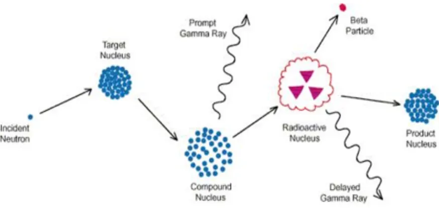
Figure 2.2 Neutron activation process. An incident neutron is absorbed by a target

nucleus and a compound nucleus is formed. The compound nucleus

emits prompt gamma ray and also a radioactive nucleus may be

formed. The radioactive nucleus emits a beta particle and delayed

gamma rays………...

12  

Figure 2.3 Range of the resistivity and conductivity for insulators,

semiconductors, and conductors. Semiconductors are in the shaded

region. [15]………

13  

Figure 2.4 The picture of the High Purity Germanium Detector in Burlington

Laboratory at NCSU. The detector cryostat is inserted into the liquid

nitrogen dewar below. The detector housing contains the germanium

crystal and a solid-state preamplifier all cooled to −196!_{C…………....}  

15  

Figure 2.5 Another picture of the HPGe Gamma Detector used in Burlington

Laboratory at North Carolina State University……….

17  

Figure 2.6 The level scheme for the decay of Bismuth-214 to Polonium-214. The

first excited state of Polonium-214 is at 609.3 keV………..

19  

Figure 2.7 Nuclear Instrumentation Module (NIM) bin, which contains a high

voltage power supply, a Gamma Spectroscopy Research Amplifier, and

a Canberra Multiport Multi-Channel Analyzer (MCA). The picture

shows the electronics for three parallel detector systems……….

21  

Figure 2.8 Genie 2000 3.2 software used to analyze the MCA spectra………. 22  

Figure 2.9 Chart of Nuclides and color code of the interactive chart of nuclides.

Half-lives of the elements are stated in seconds………...

24  

Figure 2.10 A picture of a sample page of the data collected in the Burlington

Laboratory at North Carolina State University over a 17-year period….

Figure 3.1 SAS output: The raw data for the 42% efficiency detector. The data

collection starts from 1996 and ends in 2013………...

29  

Figure 3.2 SAS output: The data set created by subtracting yearly means from the

data of Figure 3.1. The resulting data set has zero yearly mean………...

30  

Figure 3.3 SAS Output: A plot of the detrended data of Figure 3.2 and fitted

sinusoids using the fundamental (one cycle/year, 365.25 days/year) and

one harmonic (two cycles/year, (365.25)/2 days/year). The red line (the

fit) is not smooth due to the small harmonic term………

36  

Figure 4.1 The graph of the comparison between variation in the data (red curve)

and the earth-sun distance (blue curve). The x-axis represents the 12

months of a year and the y-axis represents percentage of the amplitude.

The observed variation is smaller, and not in phase with the variation in

the earth-sun distance………

39  

Chapter 1

Introduction

1.1 Introduction to Radioactivity

Radioactivity was for the first time discovered by H. Becquerel in 1896 and with the

nuclear atom theory of E. Rutherford in 1911, studies made in this field gained speed.

Radioactivity can be defined as a process where an unstable element is transformed to a

stable and different element physically and chemically by releasing various particles or

emitting radiation. Unstable nuclei are transformed to a more stable state by releasing

high-energy particles like alpha (α), beta (β) and gamma (γ). The α particles are Helium (_!!𝐻𝑒₎

nuclei with two neutrons and two protons. The β particles are high-energy electrons. In some radioactive processes, the products that are the opposite particles of electrons called positrons

appear. A gamma ray is a photon, typically with high energy. More detailed information

about these three kinds of radiation is given in Ref. [1]

1.2 Radioactive Decay Law

Physically, it is impossible to know when an atom in a radioactive sample will decay.

Radioactive decay occurs randomly and arbitrarily depending on time with characteristics

According to the decay law of radioactivity, λ is a constant whatever the age of the nucleus. For instance, its value for Radon is λ = 0.0075/ hour= 0.000125/ minute [2]. The decay number that occurs in unit time interval in a radioactive nucleus is defined as the decay

activity of nucleus. If there are N radioactive nuclei at time t, and in any moment dt no nuclei

are added to the sample, the number of nuclei decaying in the dt time interval will be

proportional to N.

𝑑𝑁 𝑡 =−𝜆𝑁 𝑡  𝑑𝑡

The minus sign in the equation indicates that the number of nuclei decreases with

time. By solving the differential equation above, the exponential radioactive decay law is

obtained and shown below

𝑑𝑁(𝑡)

𝑁(𝑡) = −𝜆  𝑑𝑡

𝑁 𝑡 = 𝑁_!𝑒!!"

Here, t in the equation represents time, N(t) is the number of nuclei at time t, N0 represents

the number of nuclei at the beginning (time t=0) and λ is the decay constant of the radioactive sample.

If both parts of the decay law equation are multiplied by λ, an expression for the activity is found as

𝜆𝑁 𝑡 = 𝜆𝑁_!𝑒!!"

Nλ in the expression above is called decay activity of sample and gives decay number

per unit time. It is indicated with I and its unit is decays/second.

Here; 𝐼  (= 𝜆𝑁) is the activity at time t and 𝐼_!  (= 𝜆𝑁_!) is the activity at time t = 0. [2]

The reciprocal of the decay constant, tm, is the mean life (or average life) of the

radioactive nuclei and it is stated as below

𝑡_! =1 𝜆

The method that is most widely used for representing the rate of radioactive decay is

by means of the half-life, t1/2. It can be stated as the time required for the number of

radioactive nuclei of a given kind to decay to half its initial value [3]. This time is

independent of the amount of the radioactive nuclide present, due to the exponential nature of

the decay. So if N is the set equal to !_!N0, then the corresponding time t1/2 is given by

ln1₂= −𝜆𝑡!/!

or

𝑡_!/! = ln2 𝜆 =

0.6931 𝜆

So the half-life is inversely proportional to the decay constant and also directly

proportional to the mean life, i.e.,

𝑡_!/! = 0.6931𝑡_!

1.3 Types of Decay

nucleus decays from an excited state to a lower state without any change in the type of

nucleus.

1.3.1 Alpha Decay

The nucleus emits an alpha particle consisting of two protons and two neutrons

(Figure 1.1). In this way, as seen in equation below, the atomic number of the decayed

nucleus decreases by 2 and its mass number by 4. (Atomic number of the nucleus, mass

number, and neutron number are Z, A, N respectively.) Rutherford proved that an alpha

particle is actually a He nucleus.

𝑋_!   → ! ! _𝑋! !!!!   !!! !!! _𝐻𝑒 ! !

Alpha decay is seen more frequently in nuclei of which the mass number is bigger

than 190 in general. Its energy spectrum is discrete, typically varying between 4 and 10MeV.

Beause it is a charged particle, it interacts intensely with electrons of the matter it passes

through. [4]

1.3.2 Beta Decay

Beta decay is of three kinds: beta-minus decay, beta-plus decay, and electron capture.

Beta-minus decay; if instability of a radionuclide is a result of a neutron surplus in the

nucleus, a neutron is converted into a proton and emits an electron and an anti-neutrino,

which can be shown as

𝑛→𝑝+𝑒!_+𝜈

!

The atomic number of a radionuclide that makes beta emission in this way increases

by one. This decay is called an isobaric decay as its mass number does not change as seen in

the reaction below (𝜈! is an anti-neutrino) [5].

𝑋_!   →

!

! _𝑋′

!!!  

!!!! +𝑒!+𝜈!

Schematic of beta-minus decay for Tritium is shown in Figure 1.2.

Beta-plus decay; if instability of atom is the result of lack of neutron or proton

surplus, the weak interaction converts a proton into a neutron while emitting a positron and a

neutrino, which can be shown as (𝜈! is neutrino and 𝑒! is positron)

𝑝→𝑛+𝑒!_+𝜈

!

In this way, the atomic number of the radionuclide that releases the positron decreases

by one [5].

𝑋_!  → !

! _𝑋′

!!!  

!!!! +𝑒!+𝜈!

Electron capture occurs if one of the electrons in a near orbit (K, L) is captured. The

electron and the proton combine creating a neutron and a neutrino. (It is shown in the

equation below). In this decay, no particle is released from the nucleus but the proton number

decreases by one as in positron decay. The mass number remains the same. (In the equations

below; 𝑝,𝑒!_,𝑛,𝜈

! are proton, electron, neutron, and neutrino respectively)

𝑝+𝑒! _{→ 𝑛+𝜈} ! 𝑋_!  +𝑒! _→ ! ! _𝑋′ !!!   !!!! +𝜈!

In all three beta decays stated above, though the numbers of protons and neutrons

change by one unit, their mass numbers remain constant. Particles called neutrino and

anti-neutrino are emitted by these three decays. The existence of anti-neutrinos was first proposed by

Pauli in 1930 and later, they were called neutrino by Fermi [6]. Energies of electrons released

Figure 1.3. Energy spectrum of beta decay electrons from Bismuth-214. The x-axis represents the kinetic energy in MeV and the y-axis represents intensity. The figure shows that energies of electrons have continues spectrum.

1.3.3 Gamma Decay

Alpha or beta decay often does not proceed to the ground state of a nucleus. The

nuclide that is formed in the decay may remain in a semi-stable state, which releases the

excitation energy in the form of gamma radiation. Gamma decay is seen in Figure 2.2. The

atomic number and mass number of a nuclide decaying in this manner do not change.

Half-life of gamma decay is very short when compared to other decays: less than 10-9

seconds in general. However, some meta-stable states have half-lives of an hour and even a

Figure 1.4. Gamma decay of Co-60. The atomic number and the mass number do not change in this decay mode.

1.4 Literature Review

In the past few years there have been new thoughts about nuclear decay rates. These

ideas start with Jerkins et al. [8] and Fischbach et al. [9] who find that there is a periodic

annual modulation in the decay rates measurements. Other studies argued that these changes

in nuclear decay rates were due to environmental influences and caused by other systematic

effects [10]. However the group, which started these investigations, countered that the

variations cannot be explained by environmental effects such as temperature, pressure,

humidity etc. [11].

Then these kinds of experiments are re-examined by several people. Norman et al.

[12] could not find any evidence for seasonal variation. Another study examined and found

correlation between decay rates and winter-summer changes [13]. In Cooper at al. [14] some

data are analyzed and no significant variations are found from the exponential decay. Not

subject of investigation in nuclear decay rates [13].

To study these questions further, we obtained a unique data set from the Nuclear

Reactor Program at North Carolina State University. As part of the Neutron Activation

Analysis program, daily calibrations of High Purity Germanium Detectors have been carried

out with a Radium-226 source. These calibrations extend back over 17 years.

As a result, we are able to undertake a search for seasonal variations in an unusually

complete set of decay rate data. In this thesis I present an analysis of these data, and present

some estimates of whether the seasonal effects I see could be due to Radon in the room

Chapter 2

Nuclear Reactor Program

2.1 PULSTAR Reactor and Neutron Activation Analysis Program

A nuclear reactor is a device designed to initiate, control and maintain a chain

reaction. It produces a steady flow of neutrons generated by the nuclear fission of heavy

nuclei.

The PULSTAR reactor is a 1-MW pool-type nuclear research reactor. It is in the

Burlington Laboratory at North Carolina State University and is administered by the Nuclear

Reactor Program. The fuel of the PULSTAR is 4% enriched, pin-type fuel consisting of UO!

(Uranium dioxide) pellets with Zircaloy cladding. This fuel gives the PULSTAR Reactor

response characteristics that are very similar to commercial light water power reactors. These

characteristics allow teaching experiments to measure moderator temperature and power

reactivity coefficients including Doppler feedback. In Figure 2.1 a schematic of nuclear

Figure 2.1. Schematic of PULSTAR Reactor. There are 4 types of facilities working currently. Neutron Powder Diffraction Facility (NPDF), Neutron Imaging Facility (NIF), Intense Positron Beam (IPB), Ultra-Cold

Neutron Activation Analysis is one of the most sensitive analytical methods used for

the quantitative multi-component examination of major, minor, and trace components in

samples from almost every imaginable field of technical and scientific interest. The neutron

irradiation and activation utilized by the 1-MW PULSTAR Nuclear Reactor facility (as an

intense neutron source) is shown in Figure 2.2. During neutron irradiation, some stable

isotopes of elements that form the samples are turned into radioactive isotopes by neutron

capture.

Figure 2.2. Neutron activation process.2 _{An incident neutron is absorbed by a target nucleus and a compound}

nucleus is formed. The compound nucleus emits prompt gamma ray and also a radioactive nucleus may be formed. The radioactive nucleus emits a beta particle, delayed gamma rays.

2.2 Detector and Electronics

Germanium is a semiconductor element. (See Figure 2.3 for details about

Germanium’s place in semiconductors.) It is a good material for detectors and widely used in

gamma-ray spectroscopy.

Figure 2.3. Range of the resistivity and conductivity for insulators, semiconductors, and conductors. Semiconductors are in the shaded region. [15]

Semiconductor gamma-ray detectors contain mainly some solid materials in which

electrons and holes are produced when a gamma ray is absorbed. Then an electric field in the

detectors have been the mainstay of high-resolution gamma-ray spectroscopy for almost 50

years and also why they are used in our study [16].

Its applications are found not only in nuclear physics but also in astrophysics, nuclear

nonproliferation, and medical imaging [17]. The Germanium detector used in this study is

shown in Figure 2.4 and Figure 2.5.

The PULSTAR reactor is used for doing neutron activation analysis and for that

reason people who are working in the Burlington Laboratory have been calibrating the

detectors for almost 18 years. In this research, advantage of these data sets of measurements

on HPGe Gamma Detectors (High Purity Germanium Gamma Detectors) is taken in order to

As shown in Figure 2.4 and Figure 2.5, the detector has a cylindrical shape. The

radioactive source, Radium-226 in our case, is placed in one of the plastic cases (right on the

detector) and this plastic case is put in the detector from the side. The Radium source should

be put on the middle of the cylindrical Germanium plate symmetrically. The detector shield

has a side door that should be closed while the detector is working. It also has a top cover not

shown in the picture. There is a liquid Nitrogen dewar for cooling the detector located under

When radioactive Radium-226 decays (for more information see Table 2.1) gamma

rays are emitted. By looking at the energy of the gamma ray, it can be determined what

isotopes were present. In this study, a 609.3 keV gamma ray (first excited state of

Polonium-214) means that there is Polonium-214 present after two beta decays. The decay scheme

(from Bismuth-214 to Polonium-214) is shown in Figure 2.6. Counting how many 609.3 keV

gamma rays are emitted in a fixed time tells us whether there is any variation in the beta

Figure 2.6. The level scheme for the decay of Bismuth-214 to 214. The first excited state of

Now let’s talk about the electronics used in this experiment. When the gamma rays

are detected by the Germanium crystal (solid crystal), the gamma rays ionize as positive

charges inside of the Germanium. If all of the gamma ray energy is positive then a certain

amount of current comes out the crystal. It gives a signal and it is converted to a voltage in a

preamplifier and then comes over to the MCA (multi channel analyzer). This MCA converts

that analog signal of the voltage into a digital signal, which can be displayed graphically.

Figure 2.7. Nuclear Instrumental Module (NIM) bin, which contains a high voltage power supply, a Gamma Spectroscopy Research Amplifier, and a Canbarra Multiport Multi-Channel Analyzer (MCA). The picture shows the electronics for three parallel detector systems.

Therefore the signal comes out first to the preamplifier then goes to the multi channel

analyzer, which gives a spectrum. After that point a computer program (called Genie 2000

3.2) is used. This software is a widely used program that connects the detector to electronics

to us). The bottom window shows the entire spectrum and it is just the zoomed area of the

peak part of the top window. It is called the interactive peak fit. Actually, there is a fit to the

data, which is called Gaussian fit on the top graph of the bottom window (the x-axis is energy

and the y-axis is the counts). The bottom graph of the bottom window is about residual. The

line between these two graphs in the bottom window separates the number of counts and the

residuals. We are not interested in the residuals now because the most important thing is the

number of counts used to look for the seasonal variation in this study.

2.3 Radium Beta Decay Source

As discussed in Chapter 1, if N is the number of radioactive nuclei present any time t;

the decay rate is given by

𝑑𝑁

𝑑𝑡 = −𝜆  𝑁(𝑡)

In this study we are looking into whether there is an additional term in this equation (for

example, due to the changing earth-sun distance) so that the equation should be

𝑑𝑁

𝑑𝑡 = −𝜆  𝑁 𝑡 +𝑓(𝑡)

where 𝑓(𝑡) is an unknown function of time.

The National Nuclear Data Center provides information about the basic properties of

atomic nuclei. An interactive chart of nuclides is shown in Figure 2.9. In this chart it is seen

that the x-axis shows the number of neutrons and the y-axis shows the number of protons in a

Figure 2.9. Chart of Nuclides4 _{and color code of the interactive chart of nuclides. Half-lives of the elements are} stated in seconds.

In this study, the radioactive decay process using HPGe Gamma Detector at

Burlington Laboratory is shown below in Table 2.1. Ra-226 undergoes three alpha decays

and two beta decays, and one more alpha decay before it reaches stability at Lead-210.

Table 2.1 Nuclides, Half-lives, Decay Modes, and Daughter Nuclides

Nuclide 𝐭𝟏/𝟐 Decay Mode Daughter Nucleus

Radium-226 1600.7 years Alpha Decay Radon-222

Radon-222 3.8 days Alpha Decay Polonium-218

Polonium-218 3.1 minutes Alpha Decay Lead-214

Lead-214 26.8 minutes Beta Decay Bismuth-214

Bismuth-214 19.9 minutes Beta Decay Polonium-214

Polonium-214 163 microseconds Alpha Decay Lead-210

2.4 Analysis the Spectra

In the Burlington Laboratory at North Carolina State University, energy calibration,

efficiency and resolution have been checked since 1996. The data sets have been collected

either every day or every few days. There are sets of data for eight different detectors having

efficiencies 21%, 23%, 24%, 25%, 26%, 38%, 42%, 65%.

The data set obtained from the 21% efficiency detector was collected from July 1997

to April 1999, the one obtained from the 23% efficiency detector was collected from

September 1996 to August 2003, the one obtained from the 24% efficiency detector was

collected from July 1997 to June 2003, the one obtained from the 26% efficiency detector

was collected from September 1996 to March 2002. The one obtained from the 25%

42% efficiency detector is collected from September 1996 until now, and the obtained from

the 68% efficiency detector is collected from July 2003 until now.

In this thesis, the data from the 42% efficiency detector (Figure 2.4 and Figure 2.5) is

examined and analyzed. This detector was used over the longest period of time and also had

the second highest detection efficiency. The detector was refurbished twice during the period

1996-2013.

The data collection is done to check that the Nuclear Reactor located in Burlington

Laboratory is working properly every day. A crystal (Radium-226) that emits gamma rays is

used. If the rate of the gamma rays does not change, the detector works properly. Because

radioactivity is a characteristic of the element, it does not change, so the detector should

detect the same everyday.

People working in the laboratory are collecting spectra for 300 seconds and making a

correction for lifetime versus dead time by using a program to analyze the data that subtracts

a background and fits to a peak (Figure 2.8). Then they record these counts on a piece of

paper that is shown in Figure 2.11. In this paper energy calibration, detector efficiency, and

detector resolutions are recorded. As stated earlier, only the counts from the 42% efficiency

Chapter 3

Analysis of the Data

In this chapter, data analysis will be described step by step. Because counts are not

taken everyday, the data sets are not equally spaced in time. Thus, the regression analysis is

an appropriate method to analyze the data sets due to the gaps in the date of the data

collected. In order to do the regression analysis, SAS (Statistical Analysis System) program

is used as a statistical program by following the suggestions of Prof. Dave Dickey.

First the data were written down on the Excel file with respect to counts by the date.

As stated in the previous chapter, the 42% efficiency detector started to work from

September 1996 and still continues, and in this analysis the data set until March 2013 was

used.

3.1 Results from the 42% Efficiency Detector

In Figure 3.1, the graph of the raw data is shown which needs to be cleaned and

detrended. The x-axis and the y-axis represent the time and the counts in 300 seconds

Figure 3.1. SAS output: The raw for the 42% efficiency detector. The data collection starts from 1996 and ends in 2013.

There is an obvious drop off at the end and long-term movement after 2011. The

reason for this unusual change in counts is the refurbishment of the detector. The detector

was sent out for repair in during that period. This part should be shifted prior to a least

squares analysis, using SAS. (For more information, the SAS code is in the Appendix)

Here in Figure 3.2 is a series created by subtracting yearly means as well as adjusting

have mean zero. We can now focus on the item of the interest, which is to look at the yearly

cycles.

Figure 3.2. SAS output: The data set created by subtracting yearly means from the data of Figure 3.1. The resulting data set has zero yearly mean.

Now let’s talk about how to look for a seasonal variation. There are 365.25 days in a

year. So the frequency we want to look for is

2𝜋

𝜔 is here the fundamental frequency which is one cycle per year. Then let’s create two

variables; sine1 and cosine1 (will shown as s1 and c1 respectively).

𝑠1= sin 𝜔𝑡 =sin 2𝜋𝑡

365.25 , (𝑡= 1,2,3,…,𝑛)

𝑐1=cos 𝜔𝑡 =cos 2𝜋𝑡

365.25 , (𝑡 =1,2,3,…,𝑛)

Both sin and cosine variables are needed because we need to get the amplitude (A)

and the phase shift (𝛿). Then they are lined up with the data. So we suppose to start with

𝐴  𝑠𝑖𝑛 𝜔𝑡+𝛿 =𝐴sin 𝛿 cos 𝜔𝑡 +𝐴cos 𝛿 sin 𝜔𝑡 , 𝛿= 𝑝ℎ𝑎𝑠𝑒  𝑠ℎ𝑖𝑓𝑡

     =𝛽_!  cos𝜔𝑡+  𝛽_!sin(𝜔𝑡)

Thus, the amplitude and the phase shift can be fitted to the data correctly by the

sample regression on sin 𝜔𝑡 and cos 𝜔𝑡 . (There is not just pure sine wave. If we make an

analogy; when you listen to the music and you play the middle c, which is a note, on a piano,

and also you play that middle c on a guitar, they sound different. The middle c here is the

fundamental frequency, just like 𝜔 here. But the reason that the middle c sounds different on

the piano and on the guitar, is because of the harmonics.) Then we need the harmonic, which

is a wave that has frequency 2𝜔, or 3𝜔, etc… So these harmonics go through 2 cycles per

year, or 3 cycles per year, or etc… They change the wave shape but still that wave repeats

Then we needed to check and see if we can leave some of these high frequencies out.

We leave these harmonics if they are statistically insignificant, in other words if there is not a

contribution from these harmonics. So we used a statistical test, which is the t test in order to

do this. (A t test is a kind of statistical test that has a t distribution under the null hypothesis.

It is used to fit the data set identify the model that best fits the population from which the

data were sampled. The exact t test mainly arises when the models have been fitted to the

data using the regression analysis [19].) The idea of this statistical test is that suppose there

really is not a harmonic that (for instance) is the fifth one; and seek what is the probability of

getting an estimated coefficient for this. If something is unlikely under a hypothesis then this

hypothesis is rejected. In this case; if this probability were less than 0.05 (called alpha; the

levels of significance) a value which is the traditionally agreed upon by scientists [20] we

would reject the hypothesis. More information can be found in Weisberg et al. [21]. Based on

Table 3.1. SAS output: (Coefficients for the sinusoidal components where the 0 degree angle is at the beginning of the year) Parameter Estimates. Variables consist of intercept and fundamental frequencies and all 4 pair of harmonics. DF represents degree of freedom. Parameter estimate attempts to approximate the unknown parameter using the measurements. Standard error is actually standard error of the mean; refer to estimates of the unknown quantity. T value shows that t test used as a regression procedure, calculated by program

automatically. Pr > |t| (probability of giving t value in this model) is obtained by using a table (called the t test distribution table) that scientist are agreed on.

Repeatedly, in order to test the null hypothesis that a parameter is 0 in the model, t

estimates are different from 0 or not). It appears that other variables do not substantially

improve the model fit.

As a result, if we have five of these harmonics in there, it could be a good fit to the

data. But if we leave out the last three harmonics, it is still a pretty good fit to the data.

Consequently, leaving these last three harmonics really doesn’t do much in terms of helping

the model, so we left them out.

Then let’s do a smaller model that might contain s1, c1 as the fundamental

frequencies and s2, c2 as the harmonics. According to Table 3.2, the parameters s1 and c1 are

significantly important and, the s2 and c2 harmonics are borderline, one is bigger and one is

slightly smaller. Hence these s2 and c2 harmonics can be included in the model or not, and

they are included in order to be safe.

As a result, the Pr > |t| is the probability of getting a result like this from the data in

which there is no seasonal component (as modeled by 2 sinusoids) and under the standard

regression assumptions, namely the white noise errors, most of the modeled variation (i.e. the

power spectrum) is due to the fundamental frequency with statistically significant but minor

contribution from the first harmonic. A model with the 4 harmonics and a fundamental

frequency showed no need to go beyond the fundamental and 1 harmonic.

Consequently, it is clearly understood from the s1 and c1 frequencies that there is a

yearly pattern. There is almost zero probability to see the data like this if there were no

seasonal variation. In other words, here is a very strong evidence that there is a yearly cycle.

Something repeating close to being a pure sin wave. In Figure 3.3 the red line shows the

predicted value by using the equation below.

𝑌= 0.58208−40.30413  𝑠1−44.76426  𝑐1−12.35282  𝑠2+15.29218  𝑐2

In this equation, the parameter estimate of variable intercept is 0.58208, the parameter

estimate of variable s1 is -40.30413, the parameter estimate of variable c1 is 44.76426, the

parameter estimate of variable s2 is -12.35282 and the parameter estimate of variable c2 is

Chapter 4

Possible Explanations for Seasonal Variation

There could be lots of reason for changes in the detector count rates such as the

environmental influences about the detector system, some systematic effects, changes in the

temperature, pressure, humidity, etc. But as discussed in Chapter 3, we find the variation to

be seasonal. Hence, the reason of this change in the beta decay rates is examined in this

chapter. Two possible explanations will be discussed below.

4.1 Sun-Earth Distance

There are two important distance points between the earth and the sun. One is named

the aphelion, which occurs when the earth and the sun are the farthest apart. This happens

around July 4 and the distance is approximately 152,171,522 km (or 94,555,000 miles). The

other is called the perihelion, which occurs when the earth is the nearest to the sun. This

happens around January 3 and the distance between the earth and the sun is approximately

147,166,462 km (91,455,000 miles). These numbers are calculated by using the earth’s

elliptical orbit around the sun [22,23].

In order to compare the variation in the distance due to these aphelion and perihelion

(Astronomical Unit is 149.6×10!_{𝑘𝑚= 92.956×10}!_{𝑚𝑖𝑙𝑒𝑠) [24] then r in AU is related to t}

in months by

1

𝑟!−1=

1

1−0.017cos 2𝜋 ₁₁𝑡−1 !

−1

To relate this to the SAS analysis we see the equation below, where -40.30 is the parameter

estimate for the variable s1 and -44.76 is the parameter estimate for the variable c1. The

mean of the counts is taken as 27500 and t represents the time in months.

𝑆𝐴𝑆 𝑚𝑒𝑎𝑛=

−40.3sin 2𝜋 ₁₁𝑡−1 −44.76cos 2𝜋 ₁₁𝑡−1 27500

Then by using these calculations, graphs of the time versus _!!_!−1 and _!"#$!"! can be

compared (Figure 4.1) The red line is the variation detected by using SAS, and the blue line

is the earh-sun distance variation in 12 months. We see the experimental variation we

detected is not in phase with the solar distance and has a much smaller magnitude. However,

just because they are out of phase, it does not mean that it is not still a geometric effect

associated with the motion and the wobble of the earth going around the sun. Our SAS

analysis corresponds to a phase shift of 228 degrees, or on a scale of 0-1, a phase of 0.633.

An in-phase variation with the earth-sun distance would give a phase shift about 0.008

(January 3), seemingly eliminating any association with the solar distance. However,

according to Sturrock et al. [13], the possibility of a north-south asymmetry of the flux from

the sun, owing to the tilt of the sun’s rotation with respect to the plane of the earth’s orbit

should also be considered. Combining the two possible effects, the earth-sun distance

0-0.183 or between 0.683-1 if the flux enhances the decay rate. The value we found falls

outside of that range. However, if the flux suppresses the decay rate, then the phase must fall

within the complementary range or between 0.183 and 0.063. Consequently, if the effect of

an as yet undetermined solar flux suppresses the decay rate, a possible solar-distance

explanation of the observed annual variation cannot be ruled out solely in the basis of the

data and the analysis presented.

Figure 4.1. The graph of the comparison between variation in the data (red curve) and the earth-sun distance (blue curve). The x-axis represents the 12 months of a year and the y-axis represents percentage of the amplitude. The observed variation is smaller, and not in phase with the variation in the earth-sun distance.

4.2 Radon Background in the Laboratory

Radon is a commonly occurring radioactive, colorless, odorless, tasteless, noble gas,

-­‐0.04   -­‐0.03   -­‐0.02   -­‐0.01   0.00   0.01   0.02   0.03   0.04  

1   2   3   4   5   6   7   8   9   10   11   12  

known situation, Radon can be found all over the U.S. Generally, the radon background can

be caused by the natural radioactivity of uranium in soil, rock or water. Radon gets into the

air you breathe. Here in this study, we are interested in the radon signal getting into the

detector. In fact, the radon atoms leak (in other words escape) into the room with random

directions and increase the radon background in the room/basement where the experiments

are carried out. There is a health limit of the radon background determined by United States

Environmental Protection Agency and this limit is approximately 148 Bqm-3 (equals to 4

pCi/L)5 The reason we test it for Radon is that it is the only one is in the gas phase and other

radioactive elements used in the experiment are in the solid phase. Because Radon is a gas it

expends all around the room.

To explore the Radon question further, we asked the NRP staff to perform two

additional measurements in June 2013. One is the Radon background in the room (measured

directly) and the other one is the background counts, which are from the detector with no

source presents. The Radon background in the laboratory was measured and found to be 7

Bqm-3 (G. Wicks, private communication). The measured background counts were around 30

in 300 second, associated with a very small but noticeable peak in the spectrum. This can be

compared with the annual variation seen in the SAS analysis which is of order 60 counts in

300 seconds.

The aim of the calculations that will be shown below is to test whether the radon

background in the basement is consistent with the observed seasonal variation or not.

Following the procedure from Gould et al. [26], the 609 keV gamma ray flux from the

experiment is found from

𝜙 = 𝑁  𝐸!

𝑘 𝐸_!  ∈ 𝐸_!  𝑚  𝑇

= 60 (609𝑘𝑒𝑉)

(2.84×10!!_{𝑒𝑟𝑔  𝑔}!!  _𝛾!!  _𝑐𝑚!_{)(0.2)(1,277×10}!_{𝑔)(300𝑠)} =26.4×10!!𝛾𝑐𝑚!!𝑠!!

The definitions in the equation are

𝜙 =𝑓𝑙𝑢𝑥  (𝑔𝑎𝑚𝑚𝑎  𝑟𝑎𝑦𝑠  𝑚!!_𝑠!!₎

𝑁 =𝑁𝑢𝑚𝑏𝑒𝑟  𝑜𝑓  𝑡ℎ𝑒  𝑒𝑠𝑡𝑖𝑚𝑎𝑡𝑒𝑑  𝑐𝑜𝑢𝑛𝑡𝑠   = 60  𝑖𝑛  𝑡𝑖𝑚𝑒  𝑡   300𝑠

𝐸_! =𝐸𝑛𝑒𝑟𝑔𝑦  𝑜𝑓  𝑡ℎ𝑒  𝑔𝑎𝑚𝑚𝑎  𝑟𝑎𝑦   0.609𝑀𝑒𝑉 =0.96×10!!_{𝑒𝑟𝑔𝑠}

𝑘= 𝑇ℎ𝑒  𝑐𝑜𝑢𝑛𝑡𝑠  𝑡𝑜  𝑓𝑙𝑢𝑒𝑛𝑐𝑒  𝑓𝑢𝑛𝑐𝑡𝑖𝑜𝑛  (= 2.84×10!!_{𝑒𝑟𝑔  𝑔}!!_𝛾𝑐𝑚!!₎

𝜖 =𝑃ℎ𝑜𝑡𝑜𝑝𝑒𝑎𝑘  𝑒𝑓𝑓𝑖𝑐𝑖𝑒𝑛𝑐𝑦   ~0.2

𝑚= 𝑀𝑎𝑠𝑠  𝑜𝑓  𝑡ℎ𝑒  𝑑𝑒𝑡𝑒𝑐𝑡𝑜𝑟  𝑖𝑛  𝑔𝑟𝑎𝑚𝑠

The flux 𝜙 striking the detector can be related to the radon decay rate 𝜌 by assuming

a uniform density for the Radon in a spherically symmetric room of radius rmax and

integrating over the appropriate solid angle for each volume element in the room. The result

is

𝜙 =𝜌𝑟_!"#

Now we need to substitute 26.4×10!!_𝛾𝑐𝑚!!_𝑠!! _{for 𝜙 and solve the equation for 𝜌}

(Then 𝜌 will be compared with the experimental value of the Radon background in the

room). But first 𝑟_!"# should be determined and there are two possible geometries for the

value of the 𝑟!"#.

First option is that the detector is closed by side and top. So 𝑟!"# would be the radius

of the inside of the detector and it can be taken as approximately 10cm. Solving the equation

by assuming a completely enclosed detector is shown below

𝜌= _𝑟𝜙 !"# =

26.4×10!!_𝛾𝑐𝑚!!_𝑠!!  

10𝑐𝑚 = 26.4×10!!𝛾𝑐𝑚!!𝑠!!

𝜌= 26.4×10!_𝐵𝑞𝑚!!

This value is very high compared to the EPA limit (which is around 148 Bq per cubic

meter) and not consistent with the direct measurement. So it is not a plausible estimate.

Another option is that the detector is not shielded. So for a room spherically

symmetric has the value of the 𝑟_!"# can be taken approximately 3m (=300cm). Solving the

equation by assuming the unshielded detector is shown below

𝜌= 𝜙 𝑟_!"# =

26.4×10!!_𝛾𝑐𝑚!!_𝑠!!  

300𝑐𝑚 = 8.8×10!!  𝛾𝑐𝑚!!𝑠!!

𝜌 =8.8  𝐵𝑞𝑚!!

This value is close to what was measured directly but is inconsistent with the

geometry of the detector, which is shielded. As a consequence, the modeling of Radon

variation in the room is not due to Radon unless there is an additional source or a mechanism

Chapter 5

Summary and Future Works

In this chapter, a summary of the thesis is stated and future work is defined. The

PULSTAR reactor located at North Carolina State University is the source of this study.

Radium-226 is used as a radioactive source and High Purity Germanium Detector is used for

detection of the gamma rays. The people working in the laboratory have taken the data sets

for 17 years and we take advantage of these data sets in this thesis. Analyzing the variances

and the regression method is used by SAS program. The results show that there is a yearly

cycle in the data. After doing some calculations and comparisons, no relation is found with

the Radon background in the laboratory, also no simple explanation for a relation with the

earth-sun distance in a year is found.

As a consequent, these arguments have not presented any evidence of the solar origin

yet. The most we can say is that these two possible explanations can be ruled out. We are

going to look now at the 38% efficiency detector to see if it confirm of refutes the effect we

saw with the 42% efficiency detector.

As a future study, other data sets (which are taken from the 21%, 23%, 24%, 25%,

26%, 38%, 65% efficiency detectors) should be examined and analyzed, in hope of

Another idea for the future is making a comparison between the reactors on and the

reactor off while taking data with the detector, so that changes in the background can be

REFERENCES

[1] J.K.Shultis and R.E.Faw, Fundementals of Nuclear Science and Engineering (CRC Press, Florida, 2007)] [Salvatore Califano, Pathways to Modern Chemical Physics, (Springer, New York, 2012), p.135–166.

[2] K.S. Krane, Introductory Nuclear Physics (John Wiley and Sons, New York, 1988)

[3] S. Glasstone and A. Sesonske, Nuclear Reactor Engineering (Chapman & Hall, New York, 1994), Vol.2, p. 30.

[4] J.K.Shultis and R.E.Faw, Fundementals of Nuclear Science and Engineering (CRC Press, Florida, 2007) p.77.

[5] J. M. Freeman, G. J. Clark,J. S. Ryder,W. E. Burcham,G.T.A. Squier and J.E. Draper. Accurate Fermi Beta Decay Measurements and the Magnitude of the Weak Interaction Vector Coupling Constant. Atomic Masses and Fundemental Constants 4:105-111, 1972

[6] G.F. Knoll, Radiation Detection and Measurement (Wiley, New York, 2010)

[7] M.F. L'Annunziata, Radioactivity: Introduction and History (Elsevier, Amsterdam, 2007) p.191.

[9] E.Fischbach, J.B. Buncher, J. T. Gruenwald, J.H. Jenkins, D. E. Krause and J.J. Mattes and J.R. Newport. Time-Dependent Nuclear Decay Parameters: New Evidence for New Forces? , Space Science Reviews, 145:285-335, July 2009.

[10] T.M. Semkow, D.K. Haines, S.E. Beach, B.J. Kilpatrick, A.J. Khan, K. O'Brien. Oscillations in radioactive exponential decay, Physics Letters B 675:415-419, May 2009.

[11] J.H. Jenkins, D.W. Mundy and E. Fischbach. Analysis of environmental influences in nuclear half-life measurements exhibiting time-dependent decay rates, Nucl. Inst. &

Meth. , 620:332-34, August 2010.

[12] E.B. Norman, Ed.Browne, H.A. Shugart, T.H. Joshi and R.B. Firestone. Evidence against correlations between nuclear decay rates and Earth–Sun distance, Astroparticle

Physics, 31:135-137, March 2009

[13] P.A. Sturrock, J.B. Buncher, E. Fischbach, D. Javorsek, J.H. Jenkins and J.J.Mattes. Concerning the phases of annual variations of nuclear decay, The Astrophysical

Journal, 737:65, August 2011.

[14] P.S.Cooper. Searching for modifications to the exponential radioactive decay law with the Cassini spacecraft, Astroparticle Physics, 31:267-269, March 2009.

[15] A. Owens, Compound Semiconductor Radiation Detectors (CRC Prees, Florida, 2012), p.2.

[17] E. L. Hull, R. H. Pehl, Amorphous germanium contacts on germanium detectors,

Nuclear Instruments and Methods in Physics Research Section A: Accelerators,

Spectrometers, Detectors and Associated Equipment, 538:651-656, February. 2005.

[18] S. Glasstone and A. Sesonske, Nuclear Reactor Engineering (Chapman & Hall, New York, 1994), Vol.2, p. 10.

[19] N.H. Bingham and H.D. Zeh, Regression Linear models in statistics (Springer, New York, 2010), p.33-59

[20] R.Schumacker and S.Tomek. Understanding Statistics Using, (Springer, Newyork, 2013), Chap. 7, p.137-168.

[21] S.Weisberg, Applied Linear Regression (Wiley, New York, 1985), p.29.

[22] N.A. Barricelli Preferential perihelion and aphelion distances, and planetary formation.

Earth Moon and Planets 34:1-33, January 1986.

[23] (The Council for the Central Laboratory of the Research Councils), Planetary and

Lunar Coordinates 2001-2020 (Willmann-Bell, Virginia, 2000)

[24] J.H.Shirley and R.W. Fairbridge, Encyclopedia of Planetary Sciences, (Kluwer, Dordrecht, 1997), Vol.18, p.48.

[25] C. T. Angell, A. C. Kaplan, J. D. Seelig, E. B. Norman, and M. Pedretti. Concepts in nuclear science illustrated by experiments with radon. American Journal of Physics,

[26] C.R. Gould, E.I. Sharapov, and A.A. Sonzogni. γ-ray fluxes in Oklo natural reactors.

SAS Code 1

options formdlim='' ls=80 orientation=portrait;

libname in '.';

%let pct=42pct;

data in.count&pct;

infile "&pct.Weekdays.csv" dlm=',' dsd missover firstobs=2;

input date :mmddyy10. count;

format date date9.;

If date>lag(date) then order=0; else order=1; *check for out

of order dates - errors;

run;

proc print data=in.count&pct; *check for out of order dates - errors;

where order=1;

run;

run;

ods listing close;

ods pdf file="&pct Count Data with Means and Plots.pdf";

proc means data=in.count&pct;

DM "GRAPH;CANCEL;"; ** to close the graph window; proc datasets library=work mt=cat nolist;

delete gseg;

run;

axis1 label=(h=3 a=90 'Count') value=(h=2)

minor=(n=3)

offset=(3);

axis2 label=(h=3 'Date')

value=(h=2)

minor=(n=2) offset=(3);

symbol1 c=black i=spline font= v=dot;

*symbol2 c=black i=hiloj font= v=circle;

*symbol3 c=black i=hiloj font=marker v=U; *symbol4 c=black i=hiloj font= v=square;

*symbol5 c=black i=hiloj font=marker v=P;

*symbol6 c=black i=join font= v=diamond;

*symbol7 c=black i=join font=marker v=C;

***use this to send to printer; *goptions dev=psl ftext=zapf

rotate=landscape lfactor=2;

***use this to see in window; goptions dev=win ftext=zapf

rotate=landscape lfactor=2;

proc gplot data=in.count&pct;

'01feb2011'd); format date year4.;

Title "&pct All Data Reference Lines at Oct 1,2001 and Feb

01,2011";

run;

quit;

proc gplot data=in.count&pct; where count between 26000 and

29000;

plot count*date / vaxis=axis1 haxis=axis2 href=('01oct2001'd,

'01feb2011'd);

format date year4.;

Title "&pct 26000-29000 Reference Lines at Oct 1,2001 and Feb

01,2011";

run;

quit;

Ods pdf close;

title;

SAS Code2

**models.sas;

%let pct=42pct;

ods html close;

ods listing close;

ods pdf file="&pct Models.pdf" style=journal;

title "&pct Models.pdf";

*libname in 'C:\temp\ChrisGould';

*libname in 'C:\Users\seyma\Desktop\42%SAS'; libname in '.';

Data Dave;

** (1) Remove outliers **;

set in.count&pct;

if (. <count< 26000) and (year<2003) then count=.; if count > 29000 then count=.;

lastpart = date> "01apr2011"d;

freq = 2*constant('pi')*date/365.25;

s1=sin(freq); c1=cos(freq);

s2=sin(2*freq); c2=cos(2*freq);

s3=sin(3*freq); c3=cos(3*freq); s4=sin(4*freq); c4=cos(4*freq);

s5=sin(5*freq); c5=cos(5*freq);

year = year(date);

run;

goptions reset=all;

axis1 label=(h=2 a=90 'Count')

value=(h=2)

minor=(n=3)

offset=(3);

axis2 label=(h=2 'Date')

value=(h=2)

minor=(n=2);

symbol1 c=black i=spline font= v=dot; *symbol2 c=black i=hiloj font= v=circle;

*symbol3 c=black i=hiloj font=marker v=U;

*symbol4 c=black i=hiloj font= v=square;

*symbol5 c=black i=hiloj font=marker v=P;

*symbol6 c=black i=join font= v=diamond; *symbol7 c=black i=join font=marker v=C;

***use this to send to printer; *goptions dev=psl ftext=zapf

rotate=landscape lfactor=2;

***use this to see in window; goptions dev=win ftext=zapf rotate=landscape lfactor=2;

proc gplot data=Dave; plot count*date/ vaxis=axis1

haxis=axis2;

format date year4.;

proc glm data=Dave; class year; model count = year lastpart; output out=out1 residual = count_yrmean;

proc gplot data=out1; plot (count count_yrmean)*date/

vaxis=axis1 haxis=axis2;

symbol1 v=none i=join c=black;

format date year4.; run; quit;

**(3) Compute spectrum using sinusoids;

proc reg data=out1; model count_yrmean=s1 c1 s2 c2 s3 c3 s4 c4

s5 c5;

Harmonics2: test s3=0, c3=0, s4=0, c4=0, s5=0, c5=0; run;

** (4) It seems harmonics 3 through 5 are not needed. Refit

and test;

proc reg data=out1; model count_yrmean=s1 c1 s2 c2; output out=out2 predicted = P;

run;

proc gplot; plot (count_yrmean p)*date/overlay vaxis=axis1

haxis=axis2;

symbol1 v=none i=join c=black w=1; symbol2 v=none i=join c=red w=3;

format date year4.;

run;

** (5) Try ARMA(1,1) error term;

proc arima data=out1;

i var=count_yrmean crosscor = (s1 c1);

run; quit; ods pdf close;

ods listing;