DEVELOPMENT OF DATA MODIFICATION METHOD FOR OPTIMIZATION OF FORECASTING PERFORMANCE
SEYEDNAVID SEYEDI
A project report submitted in partial fulfilment of the requirements for the award of the degree of Master of Engineering (Industrial Engineering)
Faculty of Mechanical Engineering Universiti Teknologi Malaysia
iii
Thanks God to enable me performing this research, I would like to dedicate this dissertation to my beloved parents and my dear sister and brother for their continuous
iv
ACKNOWLEDGEMENTS
I praise Allah, continuously, though the praise of the fervent does not do justice to His glory.
I wish to express my sincere appreciation to my supervisor, Dr. Syed Ahmad Helmi bin Syed Hassan for his guidance, advices and encouragement. His support was really assisted me until the project have been presented completely.
v
ABSTRACT
Dynamic nature of influencing parameters on market variations prevents decision makers to have a broad vision about possible future changes as an important factor in an organization survival. A precise forecast of both price and demand is a vital issue to illustrate market changes, and prosperity of plans and investments. The main purpose of this study is to develop a quantitative method, which encompasses human user cognition in order to modify timeseries, before being used as an input for forecast models. Some studies conclude ARIMA-ANN hybrid model as the best forecasting model in comparison with its individual models. However, this claim is rejected in some cases. It is a reason to check the performance of individual models in addition to hybrid model in new cases. Historical data are collected from two case studies in manufacturing and service industries. These data are modified by the developed method. Both original and modified data are implemented as inputs for ARIMA, artificial neural network (ANN), and ARIMA-ANN forecast models. The
square errors (MSE) and mean absolute percentage error (MAPE). In both case erformance. In
vi
ABSTRAK
vii
TABLE OF CONTENTS
CHAPTER TITLE PAGE
DECLARATION ii
DEDICATION iii
ACKNOWLEDGEMENTS iv
ABSTRACT v
ABSTRAK vi
TABLE OF CONTENTS vii
LIST OF TABLES xi
LIST OF FIGURE xii
LIST OF ABBREVIATIONS xv
LIST OF APPENDICES xvi
1 INTROUDUCTION 1
1.1 Introduction 1
1.2 Background of the Study 1
1.3 Problem Statement 3
1.4 Objective of the Study 3
1.5 Scope of the Study 4
1.6 Summary of Literature 4
1.7 Expected Outcomes 5
1.8 Conceptual Framework 5
1.9 Significance of the Study 6
1.10 Organization of the Study 6
viii
2 LITERATURE REVIEW 9
2.1 Introduction 9
2.2 Time Series 9
2.2.1 Decomposition Model with Seasonal Adjustment
12
2.3 ARIMA 14
2.3.1 Checking Stationary 16
2.3.2 Unit Root Test of Stationary 16 2.3.3 Parameter Estimation and Model
Identification
19
2.3.4 Diagnostic Checking 21
2.3.5 Capture Seasonal Factor by ARIMA Model
21
2.4 Artificial Neural Network 22
2.4.1 24
2.4.2 The Perceptron 25
2.4.3 Multilayer Neural Network 26
2.4.4 The Importance of Learning Rate 30
2.4.5 ANN in Forecasting 31
2.5 Hybrid Models 35
2.6 Error and Performance 37
2.7 Conclusion 39
3 METHODOLOGY 41
3.1 Introduction 41
3.2 Data Collection 41
3.3 Data Analysis 42
3.4 ARIMA 43
3.4.1 Checking Stationary 43
ix
Identification
3.4.3 Diagnosis Checking 44
3.5 Artificial Neural Network Model Selection 45
3.6 Hybrid Model 45
3.7 Performance Improvement 46
3.8 Methods Comparison 49
3.9 Conclusion 49
4 DATA COLLECTION AND ANALYSIS 50
4.1 Introduction 50
4.2 51
4.3 Historical Data Collection 51
4.4 Data Modification 52
4.4.1 Bina Demand Data 53
4.4.2 Amazon.com Stock Price Data 55
4.5 Paint Demand Forecasting 56
4.5.1 Data Analysis 56
4.5.2 ARIMA Model for the Primary Demand 57 4.5.3 ARIMA Model for the Modified Demand 61
4.5.4 Artificial Neural Network 64
4.6 Amazon.com Stock Price Forecasting 69
4.6.1 Data Analysis 69
4.6.1 ARIMA Model for Primary Stock Price 69 4.6.2 ARIMA Model for the Modified Stock
Price
74
4.6.3 Artificial Neural Network 76
4.7 Conclusion 79
5 RESULTS, DISCUSSION AND CONCLUSION 80
5.1 Introduction 80
5.2 Bina Demand Forecasting 80
x
5.2.2 Artificial Neural Network Forecast 82
5.2.3 ARIMA-ANN Forecast 84
5.3 Amazon.com Stock Price Forecasting 86
5.3.1 ARIMA Forecast 86
5.3.2 Artificial Neural Network Forecasts 87
5.3.3 ARIMA-Neural Forecasts 89
5.4 Discussion and Conclusion 91
5.5 Recommendation for Future Studies 94
REFERENCES 95
xi
LIST OF TABLES
TABLE NO. TITLE PAGE
4.1 52
4.2 Historical data for Amazon stock price 52
4.3 Averages values and modification constant 54 4.4 Averages values and modification constant 56
4.5 MSE and BIC for each AR Parameters 59
4.6 MSE and BIC for each AR Parameters 71
5.1 ARIMA Results and Performance (Primary Demand) 81 5.2 ARIMA Results and Performance (Modified Demand) 81 5.3 Neural Network Performance (Primary Demand) 82 5.4 Neural Network Performance (Modified Demand) 83
5.5 Neural Network Forecast Accuracy 83
5.6 Hybrid Forecast (Primary Demand) 85
5.7 Hybrid Forecast (Modified Demand) 85
5.8 ARIMA Results and Performance (Primary price) 86 5.9 ARIMA Results and Performance (Modified Price) 87 5.10 Neural Network Performance (Primary Price) 88 5.11 Neural Network Performance (Modified Price) 88
5.12 Neural Network Forecast Accuracy 89
5.13 Hybrid Model Forecast (Primary price) 90
5.14 Hybrid Model Forecast (Modified Price) 90
5.15 93
xii
LIST OF FIGURES
FIGURE NO. TITLE PAGE
1.1 Theoretical Framework 7
2.1 Biological Neural Network 23
2.2 Typical ANN Architecture 23
2.3 Single-layer two-input perceptron 26
2.4 Three-layer Back-propagation 28
2.5 Three-layer Feed forward Neural Network 34
3.1 Methodology flow-chart 42
4.1 Upper and lower bounds for historical demand 54 4.2 Upper and lower bounds for modified historical
demand 55
4.3 Upper and lower bounds for historical demand 55 4.4 Upper and lower bounds for modified historical
demand 56
4.5 Run plot 57
4.6 Autocorrelation function (ACF) 58
4.7 Partial autocorrelation function (PACF) 58
4.8 Residual Plots 60
4.9 Ljung-Box result 60
4.10 ACF of Residuals 61
4.11 PACF of Residuals 61
4.12 Autocorrelation Function for Modified Demand 62 4.13 Partial Autocorrelation Function for Modified Demand 62
xiii
4.15 PACF of Modified Demand Residuals 63
4.16 Residual plots of modified demand residuals 64
4.17 Nonlinear autoregressive model 65
4.18 Open-loop Neural Network 65
4.19 Autocorrelation Plot for Primary Demand 66
4.20 Input-error Cross-correlation Diagram 67
4.21 Neural Network Performance Plot 67
4.22 Autocorrelation Plot for Modified Demand 68
4.23 Input-error Cross-correlation Diagram 68
4.24 Neural Network Performance Plot 69
4.25 Run plot 70
4.26 Autocorrelation Function (ACF) 70
4.27 Partial Autocorrelation Function (PACF) 71
4.28 Residual plots 72
4.29 Ljung-Box Result 73
4.30 ACF of Residuals 73
4.31 PACF of Residuals 73
4.32 Autocorrelation Function for the modified price 74 4.33 Partial Autocorrelation Function for the modified price 74
4.34 ACF of modified price residuals 75
4.35 PACF of modified price residuals 75
4.36 Residual Plots of modified price Residuals 75
4.37 Nonlinear Autoregressive Model 76
4.38 Open-loop Neural Network 77
4.39 Autocorrelation Plot for the primary price 78
4.40 Neural Network Performance Plot 78
4.41 Autocorrelation Plot for the modified price 78
4.42 Neural Network Performance Plot 79
5.1 Real Demand and Forecasted Values 82
5.2 Neural Network Forecasts 84
xiv
5.5 Neural Network Forecasts 88
xv
LIST OF ABBREVIATIONS
AR - Autoregressive
MA - Moving Average
ARMA - Autoregressive Moving Average
ARIMA - Autoregressive Integrated Moving Average ANN - Artificial Neural Network
MSE - Mean Squared Error
RMSE - Root Mean Squared
MAE - Mean Absolute Error
MAPE - Mean Absolute Percentage Error AVR - Average Related Variance SEP - Standard Error of Prediction
PI - Persistence Index
BIC - Bayesian Information Criterion
AIC -
ACF - Autocorrelation Function PACF - Partial Autocorrelation Function DF - Dickey-Fuller test
xvi
LIST OF APPENDICES
APPENDIX TITLE PAGE
A Historical data for Amazon.com stock price 104 B ANN advance script for Bina demand
forecasting
110
C ANN advance script for Amazon.com Stock price forecasting
113
1
CHAPTER 1
INTRODUCTION
1.1 Introduction
Artificial Neural Network (ANN) and Autoregressive Integrated Moving Average (ARIMA) forecasting models are in the spotlight in these days, because of their accuracy and ease of use. In addition to the large number of studies, more investigations are required in increasing models accuracy as well as prediction performance. This chapter explains the objectives, scopes, methodology and literature review of this project.
1.2 Background of the Study
2 Forecast utilization is a method to improve planning. A high performance, high accuracy forecast method can leads to providing direction, uncertainty reduction, waste and redundancies minimization, controlling standards, and goals establishment. This kind of forecast will alert managers if there is a change in business environment and there would be more time to evaluate and ameliorate directions and plans.
I
forces organizations to improve continuously to fulfill their customers demand. A high accuracy forecast makes the supply chain more efficient and more responsive in serving customer needs. However, many factors such as political, economic and
instability in market demand, so high level of flexibility are necessary for adapting organizations plans and strategies to new situations.
Unfortunately, significant parameters, which influence the demand, vary from one circumstance to another, as a result there is no high accurate general forecasting method for all situations. Therefore, in spite of numerous research in this field, some gaps are not covered.
In this situation, forecasting the demand as an industrial engineering tool can play a critical role in increasing organizations flexibility, productivity and performance when, it provides managers with a high accurate future prediction and illuminates the way for making decisions.
3
1.3 Problem Statement
Because of high concentration given on improving integrated quantitative forecasting methods, less attention is given to the role of visual and verbal data modification and forecasting methods in reducing forecast error. Most of the quantitative methods are too complicated or are developed for special circumstances; therefore, applying methods based on user knowledge and idea can results to easier and more common methods (Hong, 2011; Andrawis, 2011). Different groups of measurable, immeasurable, and unknown parameters influence historical data; so visual and verbal evaluation and modification of historical data before being used in forecasting could have a positive effect on forecasting.
Although some unexpected measured data are known as noise and are removed, there is no specific way to rectify the effects of temporary influencing factors. As a result, improving a method to use human user knowledge and idea in adjusting historical data before implementing in forecasting, could rise up forecasting reliability and performance without increasing model complicacy.
ARIMA, ANN and ARIMA-ANN hybrid model have been studied in different cases, while there are mismatched results based on diversity of influencing factors and studied circumstances. Consequently, the selection among these models could not be completely through literatures and it is needed to test them again for different cases.
1.4 Objectives of the Study
This study is based on the following objectives:
4 ii. Implement ARIMA, ANN, and the hybrid of ARIMA-ANN on
method will produce the best forecast.
iii. To repeat the objective (ii) with the modified data as in objective (i) and to check the effect of data modification method on forecast improvement.
1.5 Scope of the Study
Three scopes of this study are as follow:
i. BINA Paint Integration and Amazon.com are selected as two case studies, representing manufacturing and service industries.
ii. MINITAB software is implemented for ARIMA model selection and forecasting.
iii. MATLAB software is used for ANN model training and forecasting.
1.6 Summary of Literature
Some factors like missing values and unusual data, in addition to seasonality and trend existence cause variation and instability in a time series. Data pre-processing is necessary to reduce this variation and instability, before using it in forecasting models, which leads to results improvement (Zhang and Qi, 2005;Wichard, 2011).
5 diagnosis checking. Shi et al. (2012)
or Bayesian information criterion (BIC) methods instead of autocorrelation function (ACF) and partial autocorrelation function (PACF) in identifying appropriate model.
Multilayer ANN is a nonlinear forecasting model. It contains one input layer, one or more hidden layer, and one output layer. The learning ability is a significant advantage of ANN; weights are changed to make input-output behaviour in line with parameter real changes (Negnevitsky, 2005). ANN outperforms classical statistical methods and box Jenkins approach (Werbos, 1988), even though it is time consuming and it may not reach to global optimum answer (Hong et al., 2011).
Traditional models limitations encourage researchers and decision makers to combine capable forecasting models (Andrawis et al., 2011). Zhang (2003) introduced a combination of ARIMA and ANN models as a general model for both linear and nonlinear cases. Improving forecast accuracy by applying ARIMA-ANN model is concluded by Gutierrez-Estrada et al. (2007). However, Shi (2012) and Taskaya-temizel (2005) report hybrid model inability in improving the result.
1.7 Expected Outcomes
Based on literatures, it is expected that the hybrid model results to a higher level of accuracy in comparison with individual models. Furthermore, adjusting data before implementing in models will have a positive effect on model accuracy (Andrawis et al., 2011).
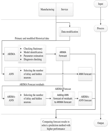
1.8 Conceptual Framework
6 and modified data are used as inputs for ARIMA, ANN and hybrid of ARIMA-ANN model. Finally, mod are compared through Mean Squared Error (MSE) and Mean Absolute Percentage Error (MAPE) to find answers for the objectives.
1.9 Significance of the Study
Having a broad view about the future changes makes planning much easier and reliable. To reach this level of reliability, forecast method accuracy has an important effect. Different statistical methods have been developed to overcome variation and instability among timeseries which are important factors for prediction exactness reduction. Though, more concentration is needed to test and improve these methods in new circumstances.
The role of pre-processing in improving a model prediction, in addition to models ability to recognize correct trend or seasonality among data have been studied. Though, number of these studies is insufficient and there is a need to add human cognition to quantitative methods. In this study a new method for pre-processing data before being applied in forecast models is introduced. This method is based on shifting out bounded data point into most possible trend intervals which are selected by user.
ARIMA and ANN can be combined as ARIMA-ANN model which is suitable for linear and nonlinear data. The hybrid model fails to outperform individual models in some cases, so its performance needs to be tested in more cases.
1.10 Organization of the Study
7 model is covered in Chapter 2; the methodology and necessary processes are represented in Chapter 3. Chapter 4 are about data collection and analysis, and the last chapter (Chapter 5) is about a summary of other chapters, results, further research works and conclusion of the study.
Manufacturing Service ARIMA ANN ARIMA-ANN Checking Stationary Model identification Parameter estimation Diagnosis checking
Selecting the number of delay and hidden neurons
ARIMA Forecast
Selecting the number of delay and hidden neurons
ARIMA-ANN forecast
Adding ANN forecast of residuals
to ARIMA forecast
ANN Forecast
Comparing forecast results to select a prediction method with
higher performance
Input
Process
Output ARIMA Forecast residuals
ARIMA Forecast Primary and modified Historical data
Data modification
8
1.11 Conclusion
95
REFERENCES
Akaike, H. (1974). Markovian representation of stochastic processes and its application to the analysis of autoregressive moving average processes. Annals of the Institute of Statistical Mathematics 26(1): 363-387.
Andrawis, R. R., Atiya, A. F., and El-Shishiny, H. (2011). Forecast combinations of computational intelligence and linear models for the NN5 time series forecasting competition. International Journal of Forecasting, 27(3), 672-688. Armstrong, J. S. (2001). Principles of forecasting: a handbook for researchers and
practitioners, Springer.
Asyraf, M. A. (2011). THE APPLICATION OF NEURAL NETWORK FOR PREDICTING HULL FORM PROPERTIES. Universiti Technologi Malaysia Bates, J. M., and Granger, C. W. (1969). The combination of forecasts. OR, 451-468. Ben Taieb, S., Bontempi, G., Atiya, A. F., & Sorjamaa, A. (2012). A review and comparison of strategies for multi-step ahead time series forecasting based on the NN5 forecasting competition. Expert systems with applications, 39(8), 7067-7083.
Bowerman, B. L., , R. T. (1987). Time series forecasting. Duxbury, Boston.
Box, G., and Jenkins, G. (1970). Time series analysis; forecasting and control. Holden-Day, San Francisco(CA).
Box, G. E. P., and Jenkins, G. M. (1976). Time Series Analysis: Forecasting, and Control. Holden Day, San Francisco, CA.
Byers, A. (2006). Jeff Bezos: the founder of Amazon.com. The Rosen Publishing Group, 46-47
Chopra, S., and Meindl, P. (2010). demand forecast in a supply chain. SUPPLY
CHAIN MANAGEMENT, PEARSON 198-226.
Crone, S. F., and Kourentzes, N. (2009). Input-variable specification for neural networks-an analysis of forecasting low and high time series frequency. Neural Networks, 2009. IJCNN 2009. International Joint Conference on, IEEE. Degeratu, V., Degeratu, S., & Schiopu, P. (2005, August). Perceptron with one layer
based on optical devices. In Advanced Topics in Optoelectronics, Microelectronics, and Nanotechnologies II (pp. 59720V-59720V). International Society for Optics and Photonics.
Dekker, M., Van Donselaar, K., and Ouwehand, P. (2004). How to use aggregation and combined forecasting to improve seasonal demand forecasts. International Journal of Production Economics, 90(2), 151-167.
96 Diaz-Robles, L. A., Ortega, J. C., Fu, J. S., Reed, G. D., Chow, J. C., Watson, J. G.,
and Moncada-Herrera, J. A. (2008). A hybrid ARIMA and artificial neural networks model to forecast particulate matter in urban areas: The case of Temuco, Chile. Atmospheric Environment, 42(35), 8331-8340.
Durbin, J., and Koopman, S. J. (2001). Time series analysis by state space methods. Oxford University Press, Oxford.
Faraway, J., and Chatfield, C. (1998). Time series forecasting with neural networks: a comparative study using the air line data. Journal of the Royal Statistical Society: Series C (Applied Statistics) 47(2): 231-250.
Fildes, R., and Makridakis, S. (1995). The impact of empirical accuracy studies on time series analysis and forecasting. International Statistical Review/Revue Internationale de Statistique: 289-308.
Franses, P. H., and Draisma, G. (1997). Recognizing changing seasonal patterns using artificial neural networks. Journal of Econometrics 81(1): 273-280. Griñó, R. (1992). Neural networks for univariate time series forecasting and their
application to water demand prediction. Neural network world 2(5): 437-450. Gutiérrez-Estrada, J. C., Silva, C., Yáñez, E., Rodríguez, N., & Pulido-Calvo, I.
(2007). Monthly catch forecasting of anchovy< i> Engraulis ringens</i> in the north area of Chile: Non-linear univariate approach. Fisheries Research, 86(2), 188-200.
Hadavandi, E., Shavandi, H., & Ghanbari, A. (2010). Integration of genetic fuzzy systems and artificial neural networks for stock price forecasting. Knowledge-Based Systems, 23(8), 800-808.
Harvey, A. C. , and GDA, P., (1979). Maximum likelihood estimation of regression models with autoregressive moving average disturbances. Biometrika 66: 49-58.
Hashem, S. (1993). Optimal linear combinations of neural networks, Purdue University. Ph.D.
Hashem, S., and Schmeiser, B. (1995). Improving model accuracy using optimal linear combinations of trained neural networks. Neural Networks, IEEE Transactions on 6(3): 792-794.
Hawkins, D. M. (2004). The problem of overfitting. Journal of chemical information and computer sciences, 44(1), 1-12.
Hippert, H. S., Pedreira, C. E., & Souza, R. C. (2001). Neural networks for short-term load forecasting: A review and evaluation. Power Systems, IEEE Transactions on, 16(1), 44-55.
Hong, W. C., Dong, Y., Chen, L. Y., & Wei, S. Y. (2011). SVR with hybrid chaotic genetic algorithms for tourism demand forecasting. Applied Soft Computing, 11(2), 1881-1890.
Hsu, S. H., Hsieh, J. J., Chih, T. C., & Hsu, K. C. (2009). A two-stage architecture for stock price forecasting by integrating self-organizing map and support vector regression. Expert Systems with Applications, 36(4), 7947-7951.
Hylleberg, S. (1992). Modelling seasonality, Oxford University Press.
Hylleberg, S. (1994). Modelling seasonal variation. Nonstationary Time Series Analysis and Cointegration, Hargreaves, CP (ed.): 153-178.
Jacobs, R. A. (1988). Increased rates of convergence through learning rate adaptation. Neural networks 1(4): 295-307.
97 Kolarik, T., and G. Rudorfer (1994). Time series forecasting using neural networks.
ACM SIGAPL APL Quote Quad, ACM.
Liu, G. Q. (2011). Comparison of Regression and ARIMA Models with Neural Network Models to Forecast the Daily Streamflow of White Clay Creek. University of Delaware
Makridakis, S., & Hibon, M. (2000). The M3-Competition: results, conclusions and implications. International journal of forecasting, 16(4), 451-476.
MINSKY, M. (1969). PAPER S., Perceptron, MIT Press, Cambridge, Mass.
Nash, J. E., and Sutcliffe, J. (1970). River flow forecasting through conceptual models part I A discussion of principles. Journal of hydrology 10(3): 282-290.
Negnevitsky, M. (2005). Artificial intelligence: a guide to intelligent systems. Addison-Wesley Longman.
Nelson, C. R., and Plosser, C. R. (1982). Trends and random walks in macroeconmic time series: some evidence and implications. Journal of monetary economics 10(2): 139-162.
Nelson, M., Hill, T., Remus, W., and O'Connor, M. (1999). Time series forecasting using neural networks: Should the data be deseasonalized first?. Journal of forecasting, 18(5), 359-367.
Pankratz, A. (1983). Forecasting with Univariate Box Jenkins Models: Concepts and Cases. John Wiley & Sons, New York.
Qi, M., and Zhang, G. P. (2001). An investigation of model selection criteria for neural network time series forecasting. European journal of operational research 132(3): 666-680.
Rosenblatt, F. (1958). The perceptron: a probabilistic model for information storage and organization in the brain. Psychological review 65(6): 386.
Rumelhart, D. E., Hintont, G. E., and Williams, R. J. (1986). Learning representations by back-propagating errors. Nature, 323(6088), 533-536. Schwarz, G. (1978). Estimating the dimension of a model. The annals of statistics
6(2): 461-464.
Sharda, R., and Patil R. B. (1992). Connectionist approach to time series prediction: an empirical test. Journal of Intelligent Manufacturing 3(5): 317-323.
Shi, J., Guo, J., and Zheng, S. (2012). Evaluation of hybrid forecasting approaches for wind speed and power generation time series. Renewable and Sustainable Energy Reviews, 16(5), 3471-3480.
Shynk, J. J. (1990). Performance surfaces of a single-layer perceptron. Neural Networks, IEEE Transactions on 1(3): 268-274.
Shynk, J. J., and Bershad, N. J. (1992). Stationary points and performance surface surfaces of a perceptron learning algorithm for a nonstationary data model. joint conference on Neural Networks, Baltimore, MD.
Slutzky, E. (1937). The summation of random causes as the sources of cyclic processes. Econometrica 5: 105-146.
Taskaya-Temizel, T., & Casey, M. C. (2005). A comparative study of autoregressive neural network hybrids. Neural Networks, 18(5), 781-789.
Ventura, S., Silva, M., Perez-Bendito, D., and Hervas, C. (1995). Artificial neural networks for estimation of kinetic analytical parameters. Analytical Chemistry, 67(9), 1521-1525.
98 Werbos, P. (1974). Beyond regression: New tools for prediction and analysis in the
behavioral sciences. Cambridge, MA., Harvard University. Ph.D.
Werbos, P. J. (1988). Generalization of backpropagation with application to a recurrent gas market model. Neural networks 1(4): 339-356.
Wichard, J. D. (2011). Forecasting the NN5 time series with hybrid models. International Journal of Forecasting 27(3): 700-707.
Yule, G. U. (1971(Published in 1927)). On a method of investigating periodicities in . (Published in 1927.) Statistical papers of George Udny Yule, A. Stuart and M. Kendall, ed., Hafer Press, New York..
Zhang, G. (1998). Linear and nonlinear time series forecasting with artificial neural networks. Kent, OH., Kent State University, . Ph.D.
Zhang, G. P. (2003). Time series forecasting using a hybrid ARIMA and neural network model. Neurocomputing 50: 159-175.