RAFIEI, AMIN. Coupled Analysis of Wave, Structure, and Sloping Seabed Interaction: Response and Instability of Seabed. (Under the direction of Dr. M.S. Rahman and Dr. M.A. Gabr).
Instability of seabed due to water surface waves may cause damage to coastal/offshore structures. Liquefaction-induced scour due to wave action may impact the stability and bearing capacity of the foundation element of coastal structures. The failure of geotextile sand containers (GSCs), as coastal protective systems, caused by instability of the foundation seabed during storm events has been reported, as for example during Hurricane Ike in 2008. Liquefaction in marine sediments may be instantaneous in which the total mean effective stress reaches zero, or it may occur due to progressive buildup of pore water pressure associated with nonlinear deformations (residual liquefaction). Of the consequences of strength degradation of soil deposit due to increase of pore pressure one is global shear failure of the entire slope in large scale. The wave-induced sliding of sloping seabed was reported after Hurricane Carla damaging South East of US. in 1961. The interaction of wave, seabed, and structure has been studied mostly for flat or midly sloping seabed (< 5°) using decoupled approach. However, some of structures may be built on or
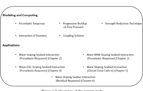
supporting marine structures are evaluated by developing a coupled finite element model in COMSOL. The interactions of all domains (fluid, structure, and seabed) are included in the analyses. Introducing such coupled approach, the extents of liquefaction around a single GSC and the loading scheme acting on the structure are obtained. The impacts of waves on global shear failure of the sloping seabed are evaluated using strength reduction technique. The effects of slope steepness (resulting in static shear stresses) on the rate of buildup of pore pressure is investigated using experimentally derived models for simulating residual response of soils under cycling.
Biot's poroelastic theory for the sediment, u-p approximation, linear waves and potential flow for the fluid, and elastodynamic equations for the structure domains are solved simultaneously in a coupled finite element model. For the global shear failure analyses, the soil is deemed as elastic-perfectly plastic with Mohr-Coulomb yield condition and associated flow rule. Residual pore pressure modellings are carried out using empirical equations based on lab data in which the models are incorporated into the analysis of wave-sloping seabed interaction.
Response and Instability of Seabed
by Amin Rafiei
A dissertation submitted to the Graduate Faculty of North Carolina State University
in partial fulfillment of the requirements for the degree of
Doctor of Philosophy
Civil Engineering
Raleigh, North Carolina 2019
APPROVED BY:
_______________________________ _______________________________ Dr. M.S. Rahman Dr. M.A. Gabr
Committee Co-Chair Committee Co-Chair
ii DEDICATION
iii BIOGRAPHY
The author was born in Behbahan, Iran, on November 19th, 1988. He graduated from Isfahan University of Technology where he received his B.Sc. degree in Civil-Structural Engineering in 2012. He earned his M.Sc. degree from University of Tehran with honors in 2015. During his M.Sc. study, the author deepened his knowledge in computational modeling of continuum media using programming. He carried out his research studies on an interdisciplinary topic “Analysis of dam-reservoir-foundation interaction due to earthquake excitation”. He joined
iv ACKNOWLEDGMENTS
The research presented in this dissertation is financially supported by the state grant from the Renewable Ocean Energy Program for the State of North Carolina through the UNC Coastal Studies Institute (CSI).
I wish to express sincere appreciation to the following individuals and organizations:
To my advisors Professor M.S. Rahman and Professor M.A. Gabr for their continuous support, guidance, and encouragements through my PhD program. It has been absolutely an honor for me to meet these wonderful people and learn a lot from them.
To other faculty members who I had the privilege to take advantage of their broad knowledge: Dr. Roy Borden, Dr. Brina Montoya, Dr. Murthy Guddati, and Dr. Alejandro Ortiz.
To North Carolina State University and UNC Coastal Studies Institute (CSI).
To my friends that I had a great time with and those who helped me through hard times of this journey, Lyndsay, Ali Marjani, Behnam, Vahid, Reza Kamali, Alireza Gharaguzlu, Hossein Ardekani, Ashkan Nafisi, Hamed, Atefeh, Jining Do, Rowshan Jadid , and many others.
v TABLE OF CONTENTS
LIST OF TABLES ... viii
LIST OF FIGURES ... ix
CHAPTER 1. INTRODUCTION ... 1
1.1. Background ... 1
1.2. Objectives ... 3
1.3. Scope ... 5
CHAPTER 2. COUPLED ANALYSIS FOR RESPONSE AND INSTABILITY OF SLOPING SEABED UNDER WAVE ACTION ... 8
Abstract ... 9
2.1. Introduction ... 10
2.2. Mathematical Model: Formulation ... 12
2.2.1. Wave-Seabed Interaction: Coupling of the Responses ... 13
2.2.2. Governing Equations of Flow ... 13
2.2.3. Equations Governing Seabed Response... 14
2.2.4. Boundary Conditions for Fluid Domain ... 16
2.2.5. Boundary Conditions for Soil Domain ... 21
2.2.6. Soil Instability: Instantaneous Liquefaction ... 22
2.2.7. Coupled Analysis: Steps ... 25
2.3. Numerical Results and Discussion... 26
2.3.1. Model Verifications for Horizontal Seabed: Decoupled Approach ... 26
2.3.2. Horizontal Seabed: Fully Coupled Approach ... 28
2.3.3. Sloping Seabed: Decoupled vs. Fully Coupled Approach ... 28
2.3.4. Effect of Slope Steepness on Seabed Response ... 30
2.3.5. Effect of Sediment Permeability and Degree of Saturation on Hydrodynamic Pressure ... 32
2.3.6. Wave-Induced Instantaneous Liquefaction... 33
2.3.7. Model Verification for Horizontal Seabed: Instantaneous Liquefaction ... 33
2.3.8. Effect of Slope Steepness on Zones of Instantaneous Liquefaction ... 34
2.4. Conclusions ... 34
CHAPTER 3. RESPONSE AND INSTABILITY OF SLOPING SEABED SUPPORTING MARINE STRUCTURES: WAVE-STRUCTURE-SOIL INTERACTION ANALYSIS ... 49
Abstract ... 50
3.1. Introduction ... 51
3.2. Mathematical Model ... 54
3.2.1. Wave-Structure-Seabed Interaction: Almost Fully Coupled Response ... 54
3.2.2. Equations Governing the Fluid Flow ... 54
vi
3.2.4. Equations Governing Seabed Response... 56
3.2.5. Boundary Conditions for Fluid Domain ... 58
3.2.6. Boundary Conditions for Soil Domain ... 62
3.2.7. Boundary Conditions for Structure and Footing Domains ... 63
3.2.8. Instantaneous Liquefaction Analysis ... 63
3.2.9. Steps of Computing the Coupled Response ... 65
3.3. Numerical Results and Discussion... 65
3.3.1. Model Verifications for the Case of Horizontal Seabed ... 66
3.3.2. Sloping Seabed Response: Fully Coupled Solution... 67
3.3.3. Effect of Slope Steepness on Seabed Response ... 70
3.3.4. Effect of Sediment Permeability and Degree of Saturation on Hydrodynamic Pressure ... 71
3.3.5. Effect of Structure’s Dimensions on Hydrodynamic Pressure Distribution ... 72
3.3.6. Evaluation of Wave-Induced Instantaneous Liquefaction ... 73
3.3.7. Effects of Wave Height on Liquefaction Zones ... 73
3.3.8. Effects of Seabed Slope Angle on Liquefaction Extent... 74
3.4. Conclusions ... 75
CHAPTER 4. WAVE-INDUCED INSTABILITY OF SEABED BENEATH GEOTEXTILE SAND CONTAINERS ... 88
Abstract ... 89
4.1. Introduction ... 90
4.2. Governing Equations ... 91
4.2.1. Fluid Domain ... 92
4.2.2. GSCs Domain ... 93
4.2.3. Seabed Domain ... 93
4.3. Boundary Conditions ... 95
4.4. Numerical Results and Discussion... 96
4.4.1. Wave-Induced Seabed Response ... 96
4.4.2. Wave-induced Instantaneous Liquefaction ... 97
4.4.3. Wave Loading on GSC ... 99
4.5. Conclusion ... 99
CHAPTER 5. WAVE-INDUCED INSTABILITY OF SLOPING SEABED: GLOBAL SHEAR FAILURE ... 105
Abstract ... 106
5.1. Introduction ... 107
5.2. Problem Description and Mathematical Model ... 111
5.2.1. Wave-Seabed Interaction: Almost Fully Coupled Response ... 111
5.2.2. Equations Governing the Fluid Flow ... 112
5.2.3. Governing Equations for Seabed ... 112
vii
5.2.5. Boundary Conditions for Soil Domain ... 118
5.2.6. The Strength Reduction Technique: Basics ... 118
5.2.7. Computation Steps ... 120
5.3. Numerical Results and Discussion... 121
5.3.1. Model Verifications ... 122
5.3.2. Sloping Seabed Response: Coupled Analysis... 123
5.3.3. Effects of Waves on Stability of the Sloping Seabed: Fully Saturated Soil ... 124
5.3.4. Effects of Waves on Stability of the Sloping Seabed: Slightly Unsaturated Soil ... 126
5.3.5. Effects of Slope Steepness on Stability of the Seabed ... 128
5.4. Conclusion ... 129
CHAPTER 6. NUMERICAL ANALYSIS OF BUILDUP OF PORE WATER PRESSURE AND DEFORMATION OF SEDIMENTS DUE TO CYCLIC WAVE ACTION ... 140
Abstract ... 141
6.1. Introduction ... 142
6.2. Mathematical Model ... 145
6.2.1. Basic Mechanics ... 145
6.2.2. Residual Pore Pressure Calculations Using Pan and Yang’s Model ... 147
6.2.3. Calculations of Residual Pore Pressure and Residual Deformations Using Bouckovalas’ Model ... 154
6.3. Numerical Results and Discussion... 157
6.3.1. Model Verification ... 157
6.3.2. Effect of Seabed Slope on Residual Pore Pressure ... 158
6.3.3. Residual Pore Pressure Calculation in Cyclic Undrained Triaxial Test ... 159
6.4. Conclusion ... 160
CHAPTER 7. SUMMARY, CONCLUSIONS, CONTRIBUTIONS, AND FUTURE WORKS ... 170
7.1. SUMMARY ... 171
7.2. Conclusions ... 173
7.3. Contributions... 174
7.4. Suggested Future Works ... 175
viii LIST OF TABLES
Table 2.1. Input data for horizontal seabed condition ... 37
Table 2.2. Input data for sloping seabed condition ... 37
Table 2.3. Input data for verification of instantaneous liquefaction ... 38
Table 2.4. Effect of slope on wave-induced momentary liquefaction ... 38
Table 3.1. Input data for horizontal seabed condition ... 78
Table 3.2. Input data for sloping seabed condition ... 78
Table 3.3. Effect of slope on wave-induced instantaneous liquefaction around the structure ... 79
Table 4.1. Input data ... 101
Table 5.1. Input data for horizontal seabed condition ... 131
Table 5.2. Input data for sloping seabed condition ... 131
Table 5.3. Wave characteristics of various storms ... 132
Table 5.4. Variations of the sloping seabed stability (FOS) within a wave cycle for different storm events ... 132
Table 5.5. Variations of the sloping seabed stability (FOS) within a wave cycle for different saturation levels (100-year Storm) ... 132
Table 6.1. Coefficient values with respect to SSR... 162
Table 6.2. Coefficient values for the function 𝑔𝑆𝑆𝑅 ... 162
ix LIST OF FIGURES
Figure 1.1. Schematic sketch of the reference problem ... 7 Figure 1.2. Overview of the current study ... 7 Figure 2.1. Schematic figure of the reference problem ... 39 Figure 2.2. Temporal variations of sediment normal stress components and their average
caused by wave action for different degree of saturation: 𝑆𝑟 = 1.0 vs. 𝑆𝑟 = 0.95 ... 40
Figure 2.3. Computation chart of the coupled model ... 41 Figure 2.4. Response comparison of the fluid domain: maximum velocity and dynamic
pressure profiles ... 41 Figure 2.5. Horizontal seabed response obtained from decoupled approach: FEM model vs. analytical solution ... 42 Figure 2.6. Variations of maximum pore water pressure (p) and dynamic pressure (𝑝𝑓)
in [Pa] ... 42 Figure 2.7. Comparison of coupled and decoupled approaches for horizontal seabed under critical wave condition: a) maximum pore water pressure, b) maximum shear stress, c) maximum vertical effective stress, d) hydrodynamic pressure
distribution along seabed surface at 𝑡 = 50 𝑠 ... 43
Figure 2.8. Problem dimensions and wave characteristics for the sloped seabed condition ... 44 Figure 2.9. Variations of shear stress with time for different mesh resolution ... 44 Figure 2.10. Sloping seabed response and comparison with decoupled approach: a) maximum pore water pressure and maximum shear stress, b) hydrodynamic pressure
x Figure 2.11. Possible comparison approaches (1 and 2) to evaluate effects of seabed steepness on the response for (a) sloping seabed with steep slope and (b) sloping seabed
with mild slope ... 45
Figure 2.12. Effect of slope on seabed response ... 46
Figure 2.13. Comparison of wave profile at 𝑡 = 7 × 𝑇 𝑠𝑒𝑐 for various slope angles ... 46
Figure 2.14. Variation of maximum hydrodynamic pressure with respect to slope magnitude for coupled and decoupled approaches ... 47
Figure 2.15. Hydrodynamic pressure difference between coupled and decoupled approach vs. a) permeability, b) degree of saturation ... 47
Figure 2.16. Instantaneous liquefied zone, FEM model vs. analytical solution [6] ... 48
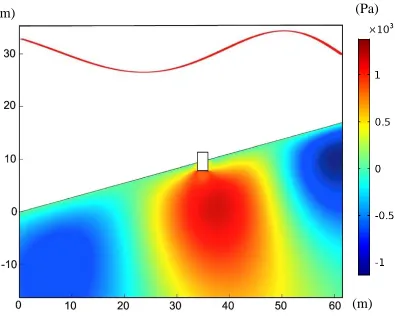
Figure 3.1. Conceptual image of the reference problem ... 80
Figure 3.2. Flowchart of the coupled analyses ... 80
Figure 3.3. Verification of fluid model: response comparison of the FE analysis vs. analytical solutions ... 81
Figure 3.4. Verification of soil model: response comparison of the FE analysis vs. analytical solutions ... 81
Figure 3.5. Model setup for sloping seabed (𝛽 = 150) ... 82
Figure 3.6. Variations of pore water pressure inside the seabed under surface waves ... 82
Figure 3.7. Variations of shear stress inside the seabed under surface waves ... 83
xi
Figure 3.9. Effect of slope on seabed response ... 84
Figure 3.10. Dynamic pressure distribution on the bed surface: Coupled (solid line) vs. Decoupled (marked points) solutions ... 85
Figure 3.11. Effects of permeability and saturation degree on hydrodynamic pressure magnitudes based on coupled and decoupled solutions ... 85
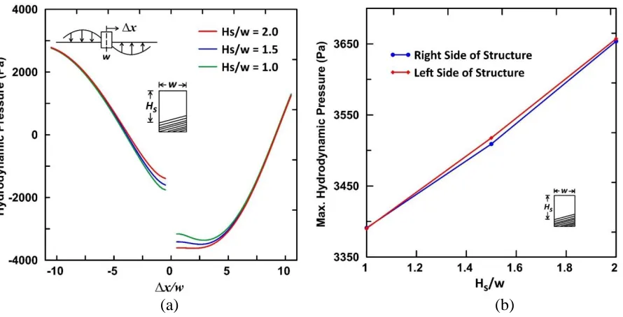
Figure 3.12. Dynamic pressure on the bed surface for various 𝐻𝑠/𝑤: (a) pressure distribution at 𝑡 = 𝑇, (b) maximum pressure at the immediate vicinity of the structure within a wave cycle ... 86
Figure 3.13. Liquefaction zones for various wave conditions: 𝐻0 = 2𝑚 and 𝐻0 = 4𝑚 ... 87
Figure 4.1. Schematic sketch of the reference problem ... 102
Figure 4.2. Model dimensions and wave characteristics ... 102
Figure 4.3. Distribution of pore water pressure and shear stress within seabed depth for points at 1.9 m distance from the centerline of the GSC ... 103
Figure 4.4. Extent of wave-induced Instantaneous liquefaction (dark blue) near the GSC at t = T for different wave heights: a) H=3 m, b) H=1.5 m ... 103
Figure 4.5. Distribution of wave loading on the GSC: a) for different times (t=T/4, T/2, t=3T/4, t=T), b) free body diagram at t=3T/4 ... 104
Figure 5.1. Schematic sketch of the reference problem ... 133
Figure 5.2. Computation chart of the coupled wave-seabed model ... 134
Figure 5.3. Computation chart for instability analyses of seabed slopes ... 134
xii Figure 5.5. Verification of soil model: response comparison of the FE analysis vs. analytical solutions ... 135 Figure 5.6. Verification of slope instability model for various slope angles and effective
friction angle: This study (Strength Reduction Finite Element Method, SRFEM) vs. Analytical solutions (Limit State Equilibrium Method)... 136 Figure 5.7. Model setup for sloping seabed (𝛽 = 150) ... 136
Figure 5.8. Distributions of maximum pore pressure and max shear stress along a vertical
line 40 𝑚 away from the right boundary of the seabed ... 137 Figure 5.9. Wave profiles for two storm conditions (Hurricane Matthew 𝐻0 = 4𝑚 and
100-year Storm 𝐻0 = 10𝑚) at times corresponding to wave trough and wave
crest above the point of interest ... 137 Figure 5.10. Effective stress paths (for point 𝑋) related to the wave crest and wave trough
for various wave heights: Hurricane Matthew 𝐻0 = 4𝑚 and 100-year Storm
𝐻0 = 10𝑚 ... 138
Figure 5.11. Demonstration of wave-induced potential failure planes of the sloping seabed under 100-year Strom at 𝑡 = 𝑇/4 ... 138 Figure 5.12. Effective stress paths (for point 𝑋) related to the wave crest and wave trough for various saturation levels: 𝑆𝑟 = 1.00 (solid blue line) and 𝑆𝑟 = 0.95
(dashed red line) ... 139 Figure 5.13. Demonstration of minimum FOSgw for various slope angles and impacts of
xiii Figure 6.3. Effect of static shear stress on residual pore water pressure, 𝑃′0 = 100 𝐾𝑃𝑎:
a) without static shear stress, b) with static shear stress 𝜏𝑠 = 50 𝐾𝑃𝑎 (After
Pan and Yang 2018) ... 164 Figure 6.4. Effect of static shear stress on residual axial strain, 𝑃′0 = 100 𝐾𝑃𝑎: a) without static shear stress, b) with static shear stress 𝜏𝑠 = 50 𝐾𝑃𝑎 (After Pan and Yang
2018) ... 164 Figure 6.5. Variations of limiting pore pressure ratio with static shear stress ratio (After Pan and Yang 2018) ... 165 Figure 6.6. Normalized pore pressure ratio as a function of normalized cycle number for a) isotopically consolidated sand, b) various SSR magnitudes (After Pan and Yang 2018) ... 165 Figure 6.7. Distribution of coefficients a and b with respect to SSR ... 166 Figure 6.8. Variations of 𝑁𝑙𝑖𝑚 with the applied CSR for a range of SSR (After Pan and Yang
2018) ... 166 Figure 6.9. Variations of coefficients 𝑎1 and 𝑏1 with SSR ... 166 Figure 6.10. Variation of coefficients 𝑎1 and 𝑏1 with SSR: predicted trend vs. known values . 167
Figure 6.11. Variations of static shear stress ratio with ground steepness ... 167 Figure 6.12. Comparison of pore water pressure with experimental results (Sumer et al.
2012): a) Variation of total (light blue color) and residual pore pressure (red color) with time for a generic point at z = 8.5 cm from soil surface,
1 CHAPTER 1. INTRODUCTION
1.1. Background
Instability of the seabed, caused by the gravitational and environmental (oceanic) forces (waves, tides and currents), and erosion (scour) are of significant concerns as they may endanger the stability and performance of coastal and offshore structures such as buried pipelines, offshore platform, Geotextile Sand Containers (GSCs), and Marine Hydrokinetic (MHK) devices. Wave-induced seabed instability has been identified as a major cause of damage to such structures [1-3]. Submarine landslide is another factor destabilizing the soil deposits and needs to be considered when the offshore facilities are built on a sloping seabed.
Based on the wave characteristics in the intermediate to shallow depth of ocean, the magnitude of the hydrodynamic pressure on seabed surface can be large enough to induce high pore pressure (the general sketch of the reference problem is shown in Figure. 1.1). Consequently, the effective stresses may be diminished resulting in a considerable loss of soil strength and possible instantaneous liquefaction in the extreme cases. Liquefaction in marine sediments may be instantaneous in which the total mean effective stress reaches zero, or it may occur due to a progressive buildup of pore water pressure associated with nonlinear deformations (residual liquefaction).
2 After hurricane Katrina, numerous liquefaction-induced scour cases around the foundation of coastal structure led to substantial damages [4]. Moreover, the initiation of sediment transport is attributed to the generated bed shear stress and the magnitude of critical shear stress. This criterion does not inherently include the gradient of pore fluid pressure in sediments. Therefore, more advanced criteria are needed to account for both aspects. Lambrechts et al. [5] proposed a model based on experimental and field observations to include the effects of stress state in sediments on sediment transport.
With the aim of maintaining the development and sustaining the environment we need to exploit all the available sources of energy transitioning from non-renewable sources to renewable. It is estimated that 33% of the total electricity usage in US can be supplied by ocean renewable energy [6], with the energy from waves providing the largest share [7]. Generally, offshore foundation elements can potentially be built on sloping seabed. This is particularly the case for MHKs deployed near the edge of Continental Shelf with steep slopes; a location where strong Gulf Stream currents are available for exploiting the water kinetic energy. The seabed stability near the foundations of these structures is as significant factor impacting their performance that is must be investigated.
The interaction of wave, seabed, and structure has been studied mostly for flat or mildly sloping seabed (< 5°) using a decoupled approach. However, as mentioned earlier, some of structures may
3 from simplified analytical solutions. The wave-induced strength degradation of soil deposit has been analyzed by assuming prescribed wave loading amplitudes on the bed surface (that is not influenced by the soil response). Yet, reduction of soil stiffness may cause smaller stress magnitudes transferred to the soil. Therefore, considering all the mentioned aspects, there is a need to study the interaction of wave-structure-sloping seabed using coupled analyses.
1.2. Objectives
The objective of this study is to investigate the response and instability of a sloping seabed (with significant slope angles) due to wave action near the foundation of marine structures following a coupled approach. To this end, first, a modeling framework to analyze the interaction of coupled media including fluid, solid, and soil is developed by implementing governing equations and boundary conditions in mathematical module of COMSOL. Then, the developed numerical framework is employed to study few marine geotechnical problems, as for instance wave-induced liquefaction analysis of sediments around a marine structure built on sloping seabed.
The interactions among media (fluid, structure, and soil) is modeled rigorously in which the influences of domains’ response on one another are included in the analyses. However, it is
4 The effects of soil and wave characteristics on the extent of instantaneous liquefaction both in free field condition and when the structure is placed on the seabed are investigated through parametric studies. Another goal of this work is to assess the liquefaction associated with progressive buildup of pore pressure. Numerical models (based on lab data) for pore pressure buildup with various levels of complications are employed. Pan and Yang’s model [8] for residual pore pressure generation (capable of including effects of static shear stresses) is incorporated in 2D plane strain analysis of wave-sloping seabed interaction. Moreover, a more advanced numerical model (based on lab data) that simulates the residual pore pressure and deformation simultaneously is used [9]. This model is employed to capture nonlinear response of soil sample in undrained cyclic triaxial test. In addition, shear failure of sloping seabed is analyzed using finite element-based shear strength reduction method which has become a more reliable approach recently because of numerous advantages over conventional limit state equilibrium methods [10].
5 1.3. Scope
This dissertation consists of seven chapters. In chapter 2, the response of finitely steep sloping seabed under surface water waves is investigated, and the development of instantaneous liquefaction is evaluated (free field). An almost fully coupled approach is employed for fluid-soil interaction that captures the coupling process among the media rigorously. Subsequently, the impacts of such coupling scheme on sediments response is assessed. The extents of instantaneous liquefaction near bed surface as a function of seabed slope angle are investigated.
In chapter 3, with the inclusion of a structure mounted on the sloping seabed, the wave-induced response of sediments around the foundation element is evaluated, and the extent of instantaneous liquefaction is computed (full system). The impacts of various coupling schemes (coupled vs. decoupled) on the response of the seabed are demonstrated.
In chapter 4, the response and instability of foundation soil around a single GSC structure under progressive surface waves are analyzed. The distribution of loading on the structure under the wave action is obtained. The extent of liquefaction around the GSC is calculated under various wave characteristics.
6 In chapter 6, the residual pore pressure response under cyclic wave loadings is investigated using experimentally-derived models. The impacts of seabed slope angle on temporal variation of pore water pressure is studied by incorporating Pan and Yang’s model [8] into coupled wave-sloping
seabed analyses. The progressive buildup of pore water pressure during undrained cyclic triaxial test is calculated (elemental behavior) employing more advanced Bouckovalas’ model [9] capable of concurrent modeling of residual pore pressure and deformation of soil elements.
Lastly, the summary, conclusion, and suggested future works are presented in chapter 7. The overview of the current study is demonstrated in Figure. 1.2.
7 Figures
Figure 1.1. Schematic sketch of the reference problem
8 CHAPTER 2. COUPLED ANALYSIS FOR RESPONSE AND INSTABILITY OF
SLOPING SEABED UNDER WAVE ACTION
The contents of this chapter have been published in the Applied Ocean Research Journal. Citation:
9 Abstract
Wave-induced instability of seabed may cause damage to coastal and offshore structures. This issue has been investigated mostly for mildly sloping (< 5°) seabed considering uncoupled
10 2.1. Introduction
Evaluation of wave-seabed interaction is required for a safe design of coastal and offshore structures such as breakwaters, buried pipelines, offshore platform, and Marine Hydrokinetic (MHK) devices. Wave-induced seabed instability, rather than construction deficiency, has been identified as a major cause of damage to such structures [1-3]. Wave action on seabed surface in intermediate water depth, may alter the stress state within the soil skeleton and pore water in such a way that seabed soil may become unstable endangering the stability of these structures [12,13]. Instability in a soil mass may be caused by either the shear stresses exceeding the shear strength or the reduction of shear strength associated with the pore pressure changes. In relation to the second cause, we identify an extreme condition of ‘liquefaction’ in which the mean effective stress
reduces to zero leading to the total loss of shear strength. Furthermore, two different types of liquefaction have been found to occur [14, 15]: (a) liquefaction due to the progressive development of pore pressure (associated with nonlinear deformation of soils and potential for accumulation of volumetric strain) due to cyclic shear stresses. (b) ‘instantaneous liquefaction’, which may occur
in nearly saturated elastic soil (with some pore air) due to phase shift in stress response. In this study our focus is only on ‘instantaneous liquefaction’.
11 results indicate a relatively good agreement between pore fluid pressure from numerical results and experimental measurements. Recently, the influence of randomness in sediment properties on liquefaction zone within the seabed, particularly the shear modulus, is investigated using stochastic finite element analysis and decoupled approach [19].
In previous studies, the wave-sloping seabed interaction is considered to be either decoupled or one-way coupled. The one-way coupled term refers to coupling of wave motion to seabed response in which there is no feedback from the soil to fluid [20]. In the work presented herein, a coupled analysis of interaction between fluid and porous seabed is considered. This accounts for the effect of fluid motion on the seabed response, and also the effect of seabed response on the motion in the fluid domain (with the wave profile kept unchanged). This should also be noted here that the continuities of both the fluid pressure and flux within the domains of fluid and porous bed are enforced at their interface.
12 In this paper, the coupled response of sloping seabed to wave action is investigated with a focus on the evaluating instantaneous liquefaction. Two main aspects investigated herein are: (a) response of seabed with significant steepness of slope, and (b) wave-seabed interaction (semi-coupled approach with known wave profile at water surface). Biot's theory, with ‘u (displacement)- p (pore water pressure)’ as field variables, is used to formulate flow and deformation response of soils [23,24] in which the acceleration of pore fluid is neglected [22], and potential flow theory [25] is used to formulate the response of fluid domain. The governing equations are solved simultaneously using finite element method. The soil sub-model is verified by available closed-form solutions for the case of horizontal seabed [22]. The extent of liquefied zone is compared to results from analytical study [16]. The effect of slope steepness on seabed response is discussed, and the effect of soil characteristics on the hydrodynamic pressure for both coupled and decoupled solutions along sloping seabed surface is investigated. A correlation between seabed slope and extent of the instantaneous liquefaction zone (width and depth) is presented. This is noted that a semi (or almost fully) coupled analysis of wave-seabed interaction together with response and instability (instantaneous liquefaction) of finitely steep seabed slopes are being considered for the first time in this study.
2.2. Mathematical Model: Formulation
13 2.2.1. Wave-Seabed Interaction: Coupling of the Responses
The wave-seabed interaction has been considered with various levels of idealization (e.g. Rahman [14], Jeng et al. [20]), which may be categorized as:
(a) Decoupled. In this, the response in fluid domain is evaluated first considering the seabed to be
impervious and nondeformable. Then the fluid pressure evaluated on the seabed is applied on the porous and deformable seabed to evaluate the response.
(b) One-way Coupled. In this approach, the dynamic pressure as well as water flux from the fluid
model is obtained and applied on the seabed surface. The effects of flow and deformation within the seabed on the fluid section are not considered.
(c) Semi-Coupled. The effects of wave-induced motion in the water domain on the flow and
deformation within the seabed soil domain and also their inverse (i.e. the effects of seabed response on the motion in water domain) are accounted. However, the wave profile is considered to remain unaffected. For this reason, this almost fully coupled analysis is being named as ‘semi coupled’. In this study, this approach is being used to formulate wave-seabed interaction.
(d) Fully Coupled. In this approach, in addition to considering the wave-seabed interaction as in
semi-coupled approach, the waves are initially generated by wave maker theory [25], propagated towards the zone of interest, and the effect of all the interactions on wave profile is also considered.
2.2.2. Governing Equations of Flow
14
∇2∅ = 0 (2.1)
where ∅ is velocity potential. The corresponding hydrodynamic pressure (𝑝𝑓) and velocity (𝑣𝑓)
are given by:
𝑣𝑓 = −∇∅ (2.2)
𝑝𝑓 = 𝜌𝑓𝜕∅
𝜕𝑡 (2.3)
in which 𝜌𝑓 denotes water density. For severe storm conditions, nonlinear wave idealizations will
be more realistic [26]. However, linear waves are adopted as the first approximation in this work.
2.2.3. Equations Governing Seabed Response
The seabed is assumed to be homogenous and isotropic, and the response is described by Biot’s poroelasticity equations in partly dynamic form (u-p approximation as presented by Biot [23] and Zienkiewicz et al. [24]). The flow of pore fluid inside the sediment obeys Darcy’s law and in this form the acceleration of pore water is neglected while the acceleration of solid particles is included. The combination of equilibrium and conservation of mass equations for pore water in a soil element can be written as [24]:
𝑘∇2𝑝 − 𝛾 𝑤𝑛 𝛽
𝜕𝑝
𝜕𝑡 + 𝑘 𝜌𝑓 𝜕2𝜀𝑣
𝜕𝑡2 = 𝛾𝑤
𝜕𝜀𝑣
𝜕𝑡 (2.4)
15 compressibility, unit weight, and pressure of pore water, and 𝜀𝑣 is volumetric strain of the soil element. Respectively, for partly saturated sediment, the compressibility takes the form as:
𝛽 = 1 𝐾𝑤 +
1 − 𝑆𝑟
𝑝𝑤0 (2.5)
in which 𝐾𝑤, 𝑆𝑟 and 𝑝𝑤0 represent bulk modulus, degree of saturation, and absolute water pressure,
respectively. Overall equilibrium of the soil element when the total stress is decomposed into effective stress and pore water pressure is given by:
𝜕𝜎𝑥′ 𝜕𝑥 + 𝜕𝜏𝑥𝑧 𝜕𝑧 − 𝜕𝑝 𝜕𝑥= 𝜌
𝜕2𝑢
𝜕𝑡2 (2.6)
𝜕𝜏𝑥𝑧 𝜕𝑥 + 𝜕𝜎𝑧′ 𝜕𝑧 − 𝜕𝑝 𝜕𝑧 = 𝜌
𝜕2𝑣
𝜕𝑡2 (2.7)
Here, 𝜎𝑥′ and 𝜎𝑧′ indicate the components of normal stresses, 𝜏𝑥𝑧 is shear stress, and 𝑢 and 𝑣 are
the components of displacement in horizontal and vertical directions of the soil skeleton, respectively. The total density of seabed sediment (𝜌) is expressed as:
𝜌 = 𝜌𝑓𝑛 + 𝜌𝑠(1 − 𝑛) (2.8)
in which 𝜌𝑠 and 𝑛 denote the density of soil solids and porosity. For isotropic linear elastic soil
16 𝜎𝑥′= 2𝐺 [𝜕𝑢
𝜕𝑥+ 𝜗
1 − 2𝜗𝜀𝑣] (2.9)
𝜎𝑧′= 2𝐺 [𝜕𝑣
𝜕𝑧+ 𝜗
1 − 2𝜗𝜀𝑣] (2.10)
𝜏𝑥𝑧 = 2𝐺 [𝜕𝑢 𝜕𝑧+
𝜕𝑣
𝜕𝑥] = 𝜏𝑧𝑥 (2.11)
where 𝐺 and 𝜗 are shear modulus and Poisson’s ratio. The final form of governing equations is obtained by substitution of Eqs. (2.9) – (2.11) into Eqs. (2.6) – (2.7) and is expressed as:
𝐺∇2𝑢 + 𝐺
1 − 2𝜗 𝜕𝜀𝑣
𝜕𝑥 = 𝜕𝑝 𝜕𝑥+ 𝜌
𝜕2𝑢
𝜕𝑡2 (2.12)
𝐺∇2𝑣 + 𝐺
1 − 2𝜗 𝜕𝜀𝑣
𝜕𝑧 = 𝜕𝑝 𝜕𝑧+ 𝜌
𝜕2𝑣
𝜕𝑡2 (2.13)
2.2.4. Boundary Conditions for Fluid Domain
In intermediate water depth where the magnitude of wave height is smaller than mean water depth and wavelength; the potential flow theory may be assumed. At water surface, the progressive wave profile is computed and the corresponding dynamic pressure (𝑝𝑓) is imposed as a prescribed
17 𝑝𝑓 =
𝜌𝑓𝑔𝐻
2 cos (𝐾𝑥 − 𝜔𝑡) (2.14)
where 𝐾 = 2𝜋 𝐿⁄ is wave number (L being wavelength), 𝜔 = 2𝜋 𝑇⁄ wave circular frequency (T being wave period), and 𝐻 denotes wave height.
By approaching shallower water, the wave height increases and the length decreases. For linear waves, the values of length are a function of period and water depth (d) and are obtained from the dispersion equation given by [25]:
𝜔2 = 𝑔𝐾𝑡𝑎𝑛ℎ(𝐾𝑑) (2.15)
or
𝐿 = 𝐿0 tanh (2𝜋𝑑
𝐿) (2.16)
𝐿0 =
𝑔𝑇2
2𝜋 (2.17)
where 𝐿0 represents the wave length in deep water.
A range of wave steepness in deep ocean is reported by Horikawa [28] based on field observations and is expressed as (𝐻0 denotes wave height in deep water):
0.008 ≤𝐻0
18 In shallower water based on conservation of energy, wave amplitude can be computed as:
𝐻 = 𝐻0{[1 + 4𝜋 𝑑 𝐿⁄
sinh (4𝜋 𝑑 𝐿⁄ )] tanh (2𝜋 𝑑 𝐿)}
−1/2
(2.19)
The steepness of waves grows higher as the water depth decreases. Such increase can reach to an extent where the waves start to break after a certain value. Such threshold for horizontal bathymetry is defined as:
𝐻 𝐿 ≥
1
7tanh (2𝜋 𝑑
𝐿) (2.20)
For the sloping seabed, the following empirical criterion using data from numerous experiments is adopted for the breaking wave height [29, 30]:
( 𝐻 𝑑)𝑏
= 𝑏
1 + 𝑎𝑑 𝑔𝑇2
(2.21)
where
𝑎 = 43.75(1 − exp (−19𝑚)) (2.22)
𝑏 = 1.56
1 + 𝑒𝑥𝑝(−19.5𝑚) (2.23)
19 At wave-seabed interface, the continuity of fluid pressure and flux are imposed as [21]:
𝑝𝑓 = 𝑝 (2.24)
𝑣𝑓= 𝑣𝑝𝑓 (2.25)
where 𝑣𝑝𝑓 is the velocity of pore fluid inside the sediment. The general equilibrium equation for
pore water in i direction is expressed as [24]:
− 𝜕𝑝 𝜕𝑥𝑖 + 𝜌𝑓𝑔𝑖− 𝜌𝑓𝑔𝑖 𝑘𝑖 𝜕𝑤̅𝑖 𝜕𝑡 − 𝜌𝑓 𝜕2𝑢
𝑖
𝜕𝑡2 −
𝜌𝑓 𝑛
𝜕2𝑤̅ 𝑖
𝜕𝑡2 = 0 (2.26)
in which 𝑤𝑖 is the relative average displacement of pore fluid in i direction with respect to that of
solid skeleton of the soil. For partly-dynamic form of Biot’s equations [24], the acceleration of pore fluid is neglected. The actual relative velocity is defined as 1/𝑛 × 𝜕𝑤̅𝑖⁄𝜕𝑡 where 𝑛 is soil porosity. Therefore, the actual relative pore water velocity (𝜕𝑤𝑖⁄𝜕𝑡) neglecting the gravitational body force term (𝜌𝑓𝑔𝑖) takes the form as:
𝜕𝑤𝑖 𝜕𝑡 = − 1 𝑛 𝑘𝑖 𝑔𝑖 𝜕2𝑢𝑖
𝜕𝑡2 −
1 𝑛
𝑘𝑖
𝜌𝑓𝑔𝑖 𝜕𝑝
𝜕𝑥𝑖 (2.27)
20 −𝜕∅ 𝜕𝑧 = − 1 𝑛 𝑘 𝑔
𝜕2𝑣
𝜕𝑡2 −
1 𝑛 𝑘 𝜌𝑓𝑔 𝜕p 𝜕𝑧+ 𝜕𝑣
𝜕𝑡 (2.28)
For the case of sloping seabed, the spatial derivative in Eq. (2.27) is normal gradient to the water-seabed interface.
21 A parametric study to determine the adequacy of domain length is performed to avoid the fictitious boundary effects on the fluid and soil response.
2.2.5. Boundary Conditions for Soil Domain
At the bottom of seabed with the finite depth, a rigid and impermeable base is assumed where zero displacement for the soil particles and no flow conditions are applied along the boundary
𝑢 = 𝑣 =𝑑𝑝
𝑑𝑛= 0 (2.29)
The continuity of pressure and flux at the interface of soil and water domains is introduced similar to the conditions mentioned for the fluid section, Eqs. (2.24) and (2.25). Also, zero shear stresses as well as zero normal effective stresses are generated, which is then expressed as:
𝜎𝑧′ = 𝜏𝑥𝑧 = 0 (2.30)
22 𝑢 =𝑑𝑝
𝑑𝑥 = 0 (2.31)
The domain geometry with applied boundary conditions is shown in Figure. 2.1.
2.2.6. Soil Instability: Instantaneous Liquefaction
In soils with slight unsaturation (due to the presence of air bubbles or gases) the total mean effective stresses may reduce to zero (𝑖. 𝑒. 𝜎̅′ = 0) leading to what is termed as ‘instantaneous liquefaction’. The liquefaction criterion can be expressed as:
𝜎̅′ = 0 or
𝜎̅′𝑔+ 𝜎̅′𝑤 = 0 (2.32)
The first term represents the geostatic mean effective stress and the second is wave-induced mean effective stress. For flat seabed in plane strain condition, the above equation takes the form as:
1
3[(ρt-ρf)gz(1+2K0)+(υ+1)(σ
'
x+σ'z)]=0 (2.33)
in which 𝜌𝑡 and 𝐾0 denote total density and coefficient of lateral earth pressure at rest, respectively.
For the case of sloping seabed, geostatic stresses are computed based on elasticity solutions of infinite sloping grounds [32] given by:
23 𝜎𝑔,𝑥 = 𝐾 𝛾𝑧 𝑐𝑜𝑠2𝛽 (2.35)
where
𝐾 = 𝐾0+ 𝑟𝑢(1 − 𝐾0) 𝑐𝑜𝑠2𝛽 − 𝐾
0 𝑠𝑖𝑛2𝛽
(2.36)
In the above, 𝐾0 is the coefficient of lateral earth pressure at rest for level ground, and 𝑟𝑢 is the pore water pressure ratio (𝑟𝑢 = 𝑢/𝛾𝑧).
For saturated sediment, the second term of LHS of Eq. (2.32) (𝜎̅′𝑤) is always equal to zero because
the wave-induced normal effective stresses are completely out-of-phase. Therefore, the total mean effective stress will be equal to geostatic mean effective stress (𝜎̅′ = 𝜎̅′𝑔) which has non-zero
values. However, in slightly unsaturated sediment, the smaller phase shift between wave-induced effective stresses may produce a negative value of the wave-induced mean effective stress leading to the possibility of the total mean effective becoming zero and thus the state of ‘instantaneous liquefaction’.
Okusa in an analytical study demonstrated the phase shift in the wave-induced effective stress response of partly saturated sediments by evaluating the effect of compressibility of pore fluid using Skempton parameter (𝐵) [16]. He indicated that lower Skempton parameter (corresponds to
higher compressibility of pore fluid and higher unsaturation level) leads to reduction of phase shift of wave-induced normal stress components (see Eqs. (2.38), (2.39), and (2.42)). This, in turn, can result in larger mean effective stresses caused by waves (𝜎̅′𝑤) and more pronounced instantaneous
24 As mentioned, the effect of pore fluid compressibility (𝛽) on the soil response (e.g. pore water pressure, mean effective stress) is considered using the Skempton parameter (𝐵) [16] defined as:
𝐵 = 1
1 + 𝑛𝛽/𝛼 (2.37)
where 𝛼 denotes compressibility of soil skeleton 𝛼 = 3(1 − 2𝜗) 𝐸⁄ with 𝐸 being Young’s Modulus. Eq. (2.37) indicates that for a given soil, higher compressible pore fluid leads to greater reduction of Skempton parameter and consequently more unsaturation.
The wave-induced normal effective stresses for slightly unsaturated and infinitely deep sediments are given by [16]:
𝜎′𝑥 = (1 − 𝐵′
1) exp(−𝐾𝑧) cos(𝐾𝑥 − 𝜔𝑡) − 𝐾𝑧 exp(−𝐾𝑧) cos(𝐾𝑥 − 𝜔𝑡)
−𝜗(1 − 𝐵
′ 1)
1 − 𝜗 exp (−𝜅1𝑧)cos (𝐾𝑥 − 𝜅2𝑧 − 𝜔𝑡)
(2.38)
𝜎′𝑧 = (1 − 𝐵′1) exp(−𝐾𝑧) cos(𝐾𝑥 − 𝜔𝑡) + 𝐾𝑧 exp(𝐾𝑧) cos(𝐾𝑥 − 𝜔𝑡) − (1 − 𝐵′1)exp (−𝜅1𝑧)cos (𝐾𝑥 − 𝜅2𝑧 − 𝜔𝑡)
(2.39)
in which 𝐾 and 𝜔 are wave number and wave frequency, respectively, and 𝜅1 and 𝜅2 are the roots
of
±k2+ [k4+ (𝜔/𝑐
𝑣)2]1/2
25 and 𝐵′
1 is obtained from:
1 𝐵′ 1
= 1 +𝑛𝛽
𝑚𝑣 (2.41)
where 𝑚𝑣 and 𝑐𝑣 are coefficients of compressibility and consolidation, respectively. Following the
expressions for normal stresses, the mean effective stress due to wave action takes the form as:
𝜎̅′𝑤 = (1 + 𝜗)
3 {2(1 − 𝐵
′
1) exp(−𝑘𝑧) cos(𝑘𝑥 − 𝜔𝑡)
− (1 − 𝐵′1) (1 − 𝜗)𝑒𝑥𝑝⁄ (−𝜅1𝑧)cos (𝑘𝑥 − 𝜅2𝑧 − 𝜔𝑡)}
(2.42)
For slightly unsaturated condition, 𝐵′
1 is less than unity resulting in 𝜎̅′𝑤 to have non-zero values.
Figure. 2.2 demonstrates the temporal variations of wave-induced normal effective stresses for a generic point inside the seabed for various saturation levels 𝑆𝑟 = 0.95, 𝑆𝑟 = 1.0 (𝜎′𝑚,𝑤 denotes mean effective stress due to wave action). As indicated, the mean effective stress caused be waves for fully saturated sediment deposits is equal to zero.
2.2.7. Coupled Analysis: Steps
In this study, as mentioned before, the semi-coupled approach is adopted, where equations governing the fluid (Eq. (2.1)) and seabed (Eqs. (2.4), (2.12)-(2.13)) domains are coupled based on interface conditions (Eqs. (2.24)-(2.25)) at common surface of the two media. Then, the set of equations are solved simultaneously, and at each time step all the field variables (velocity potential of fluid ∅, sediment displacement components 𝑢 and 𝑣, and pore water pressure 𝑝) are obtained
26 the impact of fluid motion on the seabed response, and conversely the impact of seabed response on the fluid motion.
2.3. Numerical Results and Discussion
The numerical model is solved using finite element method in time domain within COMSOL [33]. The governing equations and boundary conditions are introduced into the model. The equations are solved in time domain following Backward Differentiation Formulas method (BDFs) with the desirable stability properties [34].
The model is verified for the case of horizontal seabed and then the effect of slope on seabed response and development of instantaneously liquefied zone are studied.
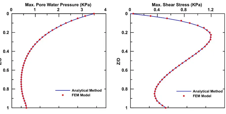
2.3.1. Model Verifications for Horizontal Seabed: Decoupled Approach
27 Regarding the seabed model verification, sediment response is obtained under a prescribed hydrodynamic pressure applied along the seabed surface (decoupled approach). The results are compared with analytical solutions [22]. The hydrodynamic pressure distribution along the bottom of the fluid domain is given as follows [25]:
𝑝𝑓(𝑥, 𝑡) = 𝑃0∗ cos (2𝜋
𝐿 𝑥 − 𝜔𝑡) (2.43)
in which
𝑃0 =
𝛾𝑤𝐻
2cosh (2𝜋𝐿 𝑑) (2.44)
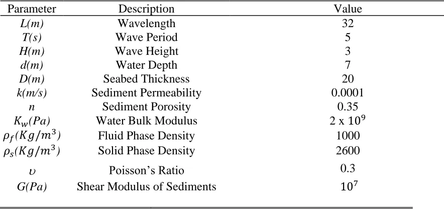
A rectangular domain with the length equal to one wavelength is modeled and the input data regarding seabed and wave characteristics are shown in Table 2.1. Rectangular elements (structured mesh) are employed for discretization of the domain and maximum element size is selected as 0.4 m after conducting a convergence analysis on mesh density.
The comparisons of solutions for maximum pore water pressure and shear stress inside the seabed depth is illustrated in Figure. 2.5. The magnitude of dynamic pressure (𝑃0) is computed from Eq.
28 2.3.2. Horizontal Seabed: Fully Coupled Approach
Fluid and soil domains for the case of horizontal seabed are modeled as coupled system, by imposing the continuity of pressure and flux. Both domains are discretized by Lagrange rectangular elements with a maximum size 0.4 m (selected after a convergence study on the mesh resolution). Also, at the interface of domains, a matching mesh is employed in which the elements of each region have the same common nodes; therefore, no data exchange mechanism is required to transfer information from one domain to another [35].
The distribution of maximum pore water pressure in sediment and maximum hydrodynamic pressure of fluid section is illustrated in Figure. 2.6 based on the data of Table 2.1. The reduction of pressure with depth and pressure continuity at the interface are apparent from Figure. 2.6. Also, as shown in Figure. 2.7, for a wide range of sediment and wave characteristics, the coupled and decoupled approaches yield approximately the same response with a very slight difference. This behavior is in concert with findings from a previous work [17] in which the maximum pore pressure obtained from the various approaches differs only by the order of 2% for a given wave condition.
2.3.3. Sloping Seabed: Decoupled vs. Fully Coupled Approach
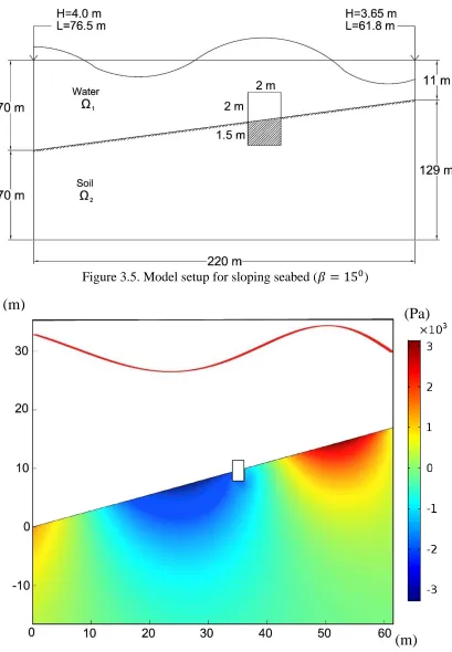
An inclined seabed with the slope of 150 is modeled, as presented in Figure. 2.8. The parameters
used in analyses are tabulated in Table 2.2. The wave height for the given wave period T=7 sec
29 intermediate water, the increase in wave height (happening in shallow water particularly) has not been observed within the given range of water depths. Also, the adopted wavelength in the deep zone is 76.5m which decreases to 61.8m based on (16). The domains are discretized by rectangular elements (near the water-sloping seabed interface) and triangle elements away from the interface. The maximum size of rectangular and triangle elements is selected as 0.2mand 2m, respectively, following parametric studies on mesh fineness. Figure. 2.9 demonstrates the temporal variations of shear stress for a generic point inside the seabed for various mesh resolution (i.e. study of size of rectangular elements near the water-seabed interface while keeping the maximum size of triangle elements constant). As shown in Figure. 2.9, there is a very slight difference (less than 2%) in the response when element size varies from 0.3m to 0.1m. As mentioned previously, the domain length is large enough to reduce the effect of the lateral boundary reflection on the system response. On the other hand, for the critical wave conditions, the unnecessary long domain generates two challenges: a) high computational costs, and, b) increase in the area of applied surface waves that results in higher induced dynamic pressure. As a consequence, the larger seabed domain is needed to avoid the multiple reflections at the boundaries. Accordingly, domain length equal to 220m is selected, which is almost three times of 𝐿0 .
30 data are compared with results from decoupled approach. As shown in Figure 2.10, the dynamic pressure becomes greater with approaching shallower water due to increase in wave steepness. In addition, for the given wave and soil characteristics, the dynamic pressure obtained from coupled and decoupled solutions are almost the same in magnitude and distribution.
2.3.4. Effect of Slope Steepness on Seabed Response
In order to investigate the impact of variation in seabed slope on system response, four slope angles of the seabed (𝛽 = 00, 𝛽 = 50, 𝛽 = 100, and 𝛽 = 150) are studied. The sediment properties in all
cases are the same and the seabed response with depth is evaluated. Two ways of comparison are possible (Figure 2.11): a comparison at two different locations but with the same water depth [see point 1 for different slope angles (a) and (b)], and a comparison at the same distance from the deep-water zone (left side of the domain) but with different deep-water depths [see point 2 for different slope angles (a) and (b)].
Regarding the first comparison, as show in Figure 2.12, by increasing the seabed slope, the maximum pore water pressure and shear stress decrease, particularly close to the seabed surface. This is similar to the results obtained by Zhang and Jeng [36]. The main reason of such behavior is related to the flow regime, particularly adjacent to the interface of the domains, and shoaling effects of waves. In the case of horizontal seabed, the flow direction is parallel to the seabed surface and water flux into the subsurface domain is insignificantly small.
31 with low permeability interface. However, by increasing the slope steepness, a higher flux between domains develops (with the normal velocity component of fluid rapidly increasing) and water percolation through the seabed is greater. This process leads to generation of smaller hydrodynamic pressure along the seabed surface and hence lower pore water pressure within the seabed sediments.
In relation to the shoaling effect, Figure 2.13 illustrates wave profile at a given time for two slope
angles 𝛽 = 150 and 𝛽 = 300 where the domain lengths are selected as 220m and 240m, respectively (selection of domain’s length is dictated by the effects of lateral boundary conditions).
As shown in Figure 2.13, for higher steepness near the wave breaking zone (on the right end), for the similar range of water depths, the wavelength is reduced significantly (higher water depth ratio 𝑑/𝐿) while the difference in wave height is not remarkable. Also, if the general form of dynamic pressure amplitude for the sloping seabed assumed to be similar to that of horizontal bed (Eq.
(2.44)), the increasing rate of denominator (cosh (2𝜋
𝐿 𝑑)) is higher than that of nominator (𝐻).
Thus, the dynamic pressure along the seabed surface for steeper slope may be smaller.
On the other hand, for points at the same distance from the deep water with various slope angles, point 2 indicated in Figure 2.11, (assuming constant wave height 𝐻0 and water depth 𝑑0 on the left
side of the domain), smaller water depth for steeper slopes results in stronger waves with more remarkable wave steepness. Therefore, the corresponding dynamic pressure on bed surface may be greater [37].
32 between the hydrodynamic pressure values obtained using both approaches as a function of slope magnitude is also shown in Figure 2.14. The shear modulus and permeability of sediment are chosen as 𝐺 = 108𝑃𝑎 and 𝑘 = 10−2𝑚/𝑠, and the same wave characteristics are applied for each
slope case. The ∆𝑃 and 𝑃0 denote the dynamic pressure difference and the pressure obtained from
decoupled approach, respectively. It is apparent that by increasing the slope magnitude, the dynamic pressure difference increases because larger flux into the seabed is developed albeit such increase is not significant.
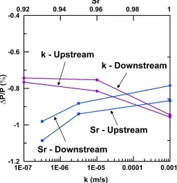
2.3.5. Effect of Sediment Permeability and Degree of Saturation on Hydrodynamic Pressure
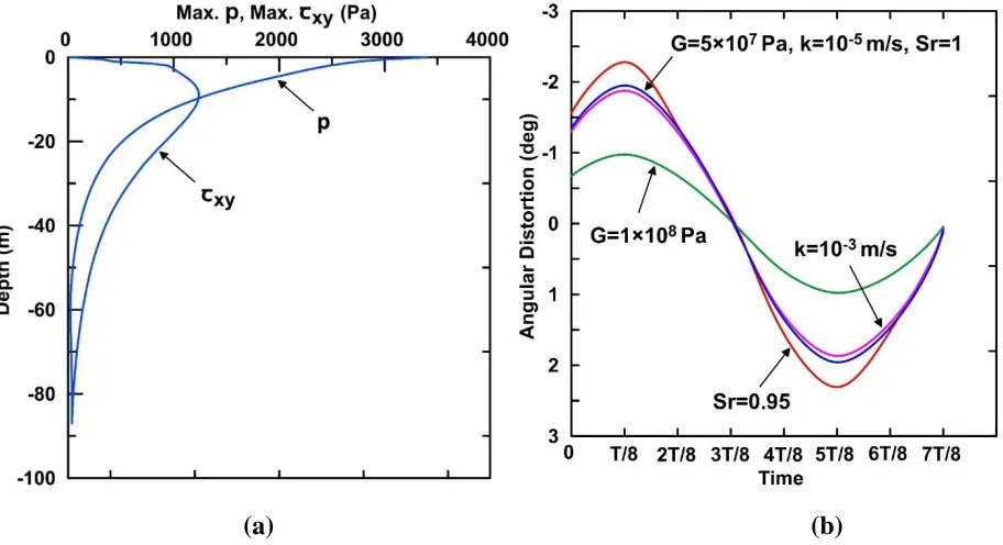
Parametric studies are performed to investigate the effect of sediment characteristics (permeability and degree of saturation) on the hydrodynamic pressure amplitude on seabed surface obtained from coupled and decoupled approaches. The variation of dynamic pressure difference with respect to sediment permeability under the same wave conditions is illustrated in Figure 2.15. A sloping seabed with the slope angle 𝛽 = 150, shear modulus 𝐺 = 108𝑃𝑎, and wave period 𝑇 = 7 𝑠𝑒𝑐 is chosen for this analysis. The hydrodynamic pressure for a generic point at 𝑥 = 200 𝑚 (Figure 2.8) on the seabed surface is obtained for three permeability values 𝑘 = 10−3 𝑚/𝑠, 𝑘 = 10−5 𝑚/𝑠, and 𝑘 = 10−7 𝑚/𝑠.
33 water flux into the seabed that causes dissipation of water energy and smaller dynamic pressure; however, such difference in amplitude is small.
Similarly, the distribution of dynamic pressure difference as a function of degree of saturation of sediments (for three saturation conditions 𝑆𝑟 = 1, 𝑆𝑟 = 0.98 and 𝑆𝑟= 0.95) is indicated in Figure 2.15 for the sloping seabed (𝛽 = 150). The same wave condition with the wave period 𝑇 = 7 𝑠𝑒𝑐 is imposed in each case, and the shear modulus and permeability of sediments are selected as 𝐺 = 5 × 10⁷𝑃𝑎 and 𝑘 = 10−5 𝑚/𝑠, respectively. As shown in Figure 2.15, slight unsaturation leads to more compressibility of the soil layer, and consequently the seabed acts as a flexible base that dissipates the water energy and reduces the dynamic pressure in comparison with the rigid base; although, such reduction is not significant.
2.3.6. Wave-Induced Instantaneous Liquefaction
In this section, the extent of liquefied zone within the horizontal seabed is obtained for a given set of soil and wave characteristics and verified by comparing to results from an analytical study [16]. Then, the effect of slope angle on the extent of liquefaction is examined.
2.3.7. Model Verification for Horizontal Seabed: Instantaneous Liquefaction
34 liquefaction may not occur. This is also noted from the results that the depth of liquefied zone within the saturated seabed is measured as nearly zero.
2.3.8. Effect of Slope Steepness on Zones of Instantaneous Liquefaction
The effect of seabed slope on extension of instantaneous liquefied zones is studied considering three slopes (𝛽 = 00, 𝛽 = 100, and 𝛽 = 150). The sediment characteristics in all cases are the
same and the liquefaction properties (width, depth, area) are evaluated under the same critical wave characteristics. It is assumed that seabed material is slightly unsaturated with the degree of saturation 𝑆𝑟 = 0.95 uniformly through the depth, and the coefficient of lateral earth pressure at rest for the horizontal seabed is assumed as 𝐾0 = 0.5.
The extent of the zone near the seabed surface, where critical wave conditions exist is indicated in Table 2.4. By increasing the slope, the wave-induced liquefied zone is getting smaller (and the corresponding depth decreases). This is because the seabed response is a function of the slope, as was shown earlier, and an increase in slope results in a decrease of induced stresses within the sediment. Therefore, in comparison with the horizontal case, at lower depth from the seabed surface the induced mean effective stress will be equal to geostatic mean stress of the seabed. Consequently, the depth of instantaneous liquefaction reduces for steeper slopes.
2.4. Conclusions
35 elastic deformation are used to formulate the model. The model is verified with analytical solutions for the case of horizontal seabed. A semi (or almost fully) coupled analysis of wave-seabed interaction together with response and instability (instantaneous liquefaction) of finitely steep seabed slopes have been considered for the first time in this study.
Based on the results obtained in this study, the following conclusions are made:
1. For the horizontal seabed, coupled and decoupled analyses yield nearly the same response. This observation is valid for a wide range of sediment properties and wave characteristics and is consistent with earlier findings.
2. For the sloping seabed, the pore water pressure, particularly close to surface, decrease with increasing slope steepness. Moreover, the shear stress amplitudes for steeper slopes appeared to be smaller. For the steeper slopes, larger water flux into the seabed and weaker wave profile lead to a lower pore pressure.
3. The coupled and decoupled analyses result in almost the same pore water pressure also in sloping seabed under critical wave conditions and various sediment properties. However, the differences in results from the two approaches become larger for steeper slopes as the flux between regions increases. Yet, the magnitude of flux into sloping bed is not large enough to produce a significant difference in seabed response.
37 Tables
Table 2.1.
Input data for horizontal seabed condition
Parameter Description Value
L(m) Wavelength 32
T(s) Wave Period 5
H(m) Wave Height 3
d(m) Water Depth 7
D(m) Seabed Thickness 20
k(m/s) Sediment Permeability 0.0001
n Sediment Porosity 0.35
𝐾𝑤(Pa) Water Bulk Modulus 2 x 10⁹
𝜌𝑓(𝐾𝑔/𝑚3) Fluid Phase Density 1000
𝜌𝑠(𝐾𝑔/𝑚3) Solid Phase Density 2600
Poisson’s Ratio 0.3
G(Pa) Shear Modulus of Sediments 107
Table 2.2.
Input data for sloping seabed condition
Parameter Description Value
T(s) Wave Period 7
k(m/s) Sediment Permeability 0.0001
n Sediment Porosity 0.35
𝐾𝑤(Pa) Water Bulk Modulus 2 x 10⁹
𝜌𝑓(𝐾𝑔/𝑚3) Fluid Phase Density 1000 𝜌𝑠(𝐾𝑔/𝑚3) Solid Phase Density 1720
Poisson’s Ratio 0.3
G(Pa) Shear Modulus of
Sediments 5 × 10
7
38 Table 2.3.
Input data for verification of instantaneous liquefaction
Water Depth (𝑚)
Wave Conditions Sediment Properties
Heigh t (𝑚) Perio d (𝑠) Lengt h (𝑚) Sedimen t type Compressibilit y (𝑚2/𝑁)
Permeabilit y (𝑚/𝑠) Poisson’ s ratio Bulk densit y (𝑡/
𝑚3) 20 5 15 197.4
2
Loose Sand
9.18 × 10⁻⁸ 10−4 0.3 1.5
Table 2.4.
Effect of slope on wave-induced momentary liquefaction
Seabed Slope (𝑑𝑒𝑔)
Width (𝑚) Depth (𝑚) Area (𝑚2)
𝛽 = 0 36.3 1.0 23.9
𝛽 = 10 36.5 0.9 16.8
39 Figures
40
41 Figure 2.3. Computation chart of the coupled model
42
Figure 2.5. Horizontal seabed response obtained from decoupled approach: FEM model vs. analytical solution
Figure 2.6. Variations of maximum pore water pressure (p) and dynamic pressure (𝑝𝑓) in [Pa]
43
(a) (b)
(c) (d)
Figure 2.7. Comparison of coupled and decoupled approaches for horizontal seabed under critical wave condition: a) maximum pore water pressure, b) maximum shear stress, c) maximum
44 Figure 2.8. Problem dimensions and wave characteristics for the sloped seabed condition
45
Figure 2.10. Sloping seabed response and comparison with decoupled approach: a) maximum pore water pressure and maximum shear stress, b) hydrodynamic pressure distribution along
seabed surface at t=50 s
46
Figure 2.12. Effect of slope on seabed response
47 Figure 2.14. Variation of maximum hydrodynamic pressure with respect to slope magnitude for
coupled and decoupled approaches
49 CHAPTER 3. RESPONSE AND INSTABILITY OF SLOPING SEABED SUPPORTING
MARINE STRUCTURES: WAVE-STRUCTURE-SOIL INTERACTION ANALYSIS
Some of the contents of this chapter have been published in the proceedings of Geo-Congress. Citation:
50 Abstract
Seabed instability due to water waves may cause significant damages to marine structures. Liquefaction-induced scour due to wave action may impact the stability and bearing capacity of the foundation element of coastal structures. The interaction of wave, seabed, and structure has been studied mostly for flat or slightly sloping seabed (< 5°). However, some of structures may
51 3.1. Introduction
Evaluation of response and instability of seabed considering wave-structure-seabed interaction is needed for a safe design of coastal and offshore facilities such as breakwaters, buried pipelines, offshore platform, and Marine Hydrokinetic (MHK) devices. Wave-induced seabed instability, rather than structural breakdown, has been identified as a major cause of damage to such structures [1-3]. After hurricane Katrina, liquefaction-induced scour around the foundation of coastal structures (resulting from soil instability due to wave action) led to substantial damages [4].
For shallower water depths, wave-induced instability of sediments within the seabed can stem from: (a) shear stress (due to wave loading on the bed surface) exceeding the shear strength of soil, and (b) reduction of shear strength caused by increase of pore water pressure as waves propagate along the water surface. Regarding the second cause, two extreme cases may occur: (i) instantaneous liquefaction in which the mean effective stress of nearly saturated sediments reaches zero as the phase shift of the normal stress components [16, 38]; (ii) the liquefaction caused by progressive buildup of pore water pressure associate with tendency of fully saturated soil elements for volume reduction under cyclic wave loadings [15]. The focus of this study is on instantaneous liquefaction of sediments around the structure.
52 the interaction of the soil and water should be fully considered; thus, the deformability and porosity of sediments influence the water flow in the fluid domain and vice versa [17].
Xiao et al. [18] in a decoupled numerical analysis indicated the high potential for failure of sloping sand beach due to tsunami-induced instantaneous liquefaction. Rafiei et al. [38] demonstrated that the extent of instantaneous liquefaction along the bed surface becomes smaller for steeper slopes. The wave characteristics can impact the extent of instantaneous liquefied zones around mounted breakwaters significantly as shown by Jeng et al. [20]. Moreover, the response of gently sloping seabed supporting a breakwater and subjected to tsunami wave loadings has been examined in an uncoupled analysis [40]. The results indicated that instantaneous liquefaction is less probable near the structure’s foundation as tsunami wave loadings induce compressional stresses in the seabed.
As mentioned, in the earlier works considered the wave-structure-seabed interaction using a decoupled or semi-coupled analysis (e.g. [20], [35]). However, the significance of using more accurate coupling scheme for response and instability of seabed around the structure’s foundation is yet to be investigated. Furthermore, offshore foundation elements may have to be built on sloping seabed. This is particularly the case for Marine Hydrokinetic (MHK) devices deployed near the edge of Continental Shelf with steep slopes, a location where strong Gulf Stream currents are available for exploiting the water kinetic energy.
53 A coupled analysis of interaction between fluid, structure, and porous sloping seabed is considered. This accounts for: (a) the effect of fluid motion on the response of structure and seabed, (b) the effect of seabed response on the motion in the fluid domain (with the wave profile kept unchanged) and on structure response (displacements and stresses), and also (c) the effect of structure response on fluid and seabed. To this end, all the interface conditions among the domains (i.e. continuity of displacement, traction, and flux) are enforced.