ATLAS Masterclasses –
W
and
Z
path physics and presentation
of the
Z
path measurement
Magnar K. Bugge1,a, Eirik Gramstad1, Vanja Morisbak1, Farid Ould-Saada1, Maiken Pedersen1,
and Silje H. Raddum1
1University of Oslo
Abstract.First, the physics behind the ATLASWandZpath Masterclass measurements is presented. Subsequently, a more detailed account of the ATLASZ path Masterclass measurement is given, with emphasis on the event identification analysis performed by the students as well as the presentation and interpretation of their results.
1 Introduction
The International Masterclasses [1, 2] is a particle physics outreach program run by the International Particle Physics Outreach Group (IPPOG) [3]. The aim of the program is to provide an opportunity for 15- to 19-year old school students to discover particle physics through hands-on measurements with real LHC data. Several different measurements are available, of which two involve ATLAS data. These two, the so-called “Wpath” and “Zpath” measurements, are the subjects of this article.
In this article, the physics behind the ATLASW andZ path Masterclass measurements will first be presented at a level suitable also for people who are not particle physics experts. Then, theZpath measurement will be described in more detail. Further information on theW path measurement is given in reference [4].
2 The Standard Model
The fundamental matter particles of the Standard Model of particle physics are the quarks and leptons. They interact via the electromagnetic, weak, and strong forces. Associated with these forces are force carrier particles, which mediate the forces between the matter particles. The electromagnetic force is mediated by the photon, the weak force is mediated by theW±andZ0 bosons, and the strong force is mediated by the gluons. Each matter particle of the Standard Model has its respective antiparticle with the same mass and opposite electric charge.
The quarks experience all the three Standard Model forces. In particular, they interact via the strong force, and they are therefore never seen as free particles. They areconfinedwithin hadrons, such as the proton, which consists of two up quarks and one down quark. The leptons experience only the electromagnetic and weak forces. The neutrinos, being electrically neutral leptons, are left
Figure 1.Plots of a PDF set (MSTW 2008, NLO) at the energy scaleQ2=10 GeV2. The shapes of the distributions of the
valence quarksu(the up quark) andd(the down quark) are seen to be different from those of the distributions of gluons and sea quarks. In particular, the distributions of the valence quarks are peaked at rather high momentum fractions. From reference [7].
interacting only via the weak force, and are therefore very hard to detect. Among thechargedleptons, we find the well known electron (e−), and a heavier “version” of the electron called the muon (μ−).
In addition to the matter and force particles, the Standard Model contains an additional particle: the Higgs boson, whose corresponding field is responsible for giving mass to most of the Standard Model particles. In particular, the Higgs field is responsible for breaking the symmetry between the weak force and the electromagnetic force, resulting in massiveW± andZ0 bosons and a massless photon. Discovered in 2012 [5, 6], the Higgs boson was the last particle of the Standard Model to be observed in experiment.
3 Proton-proton collisions
At the Large Hadron Collider (LHC), protons are collided head on at very high energy, and the par-ticles emerging from the collisions are detected by detectors, such as the ATLAS (A Toroidal LHC ApparatuS) detector. The recorded data are used to improve our understanding of nature at the small-est distance scales.
Many of the collisions between protons are in fact really collisions between individual constituents from within the protons. Such collisions are referred to ashard scatterings. As the proton consists of up and down quarks, hard scatterings between such quarks can be observed in proton-proton col-lisions. However, as the strong force between the up and down quarks in the proton is mediated by gluons, also gluons can enter the hard scatterings. Finally, as gluons can “split” into quark-antiquark pairs, the proton consists effectively of both the up and down quarks (calledvalencequarks), gluons, and additional quarks and antiquarks from gluon splittings (calledseaquarks).
The Parton Density Functions (PDFs) describe how often each of the various proton constituents will go into a hard scattering with a given momentum fractionx(the fraction of the proton momentum carried by the constituent). They summarize the proton structure as seen on a given energy scale. The PDFs of the proton at low energy are shown in figure 1. The shapes of the distributions of the valence quarksu(the up quark) andd(the down quark) are seen to be different from those of the distributions of gluons and sea quarks.
pos-Figure 2.Feynman diagrams showing the production and subsequent decay into leptons of theW±andZ0bosons in
hard scatterings in proton-proton collisions.
itively chargedW+ boson, or a down quark and an up antiquark may collide to form a negatively chargedW−boson. An up or down quark may collide with its respective antiquark to form an elec-trically neutralZ0boson. TheW±andZ0bosons are short lived (with lifetimes of the order 10−25s), and decay in practice immediately after their creation. They can therefore only be observed via their decay products, and decays into leptons are ideal for such detection. TheFeynman diagramsin fig-ure 2 show schematically the production and subsequent decay into leptons of theW±andZ0bosons in hard scatterings in proton-proton collisions.
The decays of theW±andZ0bosons into leptons provide characteristic experimental signatures. The decay of theZ0 boson into a pair of oppositely charged leptons gives such a pair among the particles emerging from the collision (among thefinal stateparticles), where each lepton will typically have a large momentum component perpendicular to the direction of motion of the colliding protons (perpendicular to thebeam line). The decay of aW+orW−boson into a charged lepton and a neutrino gives one charged lepton with a large momentum component perpendicular to the beam line. In addition, there will be a momentum imbalance in the plane perpendicular to the beam line due to the neutrino, which experiences only the weak interaction, and is therefore not measured directly by the detector. This momentum imbalance motivates the calculation of an experimental quantity called themissing transverse energy, which can be thought of as an indirect measurement of the neutrino’s momentum component in the plane perpendicular to the beam line.
The Higgs boson may also be produced in a proton-proton collision via a hard scattering of two gluons. This process is much more rare than the production ofW±andZ0 bosons. Some Feynman diagrams for the production and decay of the Higgs boson in proton-proton collisions are shown in figure 3. Note that both the production of the Higgs boson and its decays into photons and leptons happen via intermediate states of heavy particles. This is the top quark in the case of production, and theW±andZ0bosons in the case of the decays. The reason for this is that the Higgs boson interacts primarily with heavy particles, and theW±andZ0bosons and the top quark are the heaviest particles of the Standard Model. This also explains why Higgs production at the LHC is much more rare than W±andZ0boson production: the quarks inside the proton are very light, and their direct coupling to the Higgs boson is therefore very weak.
Figure 3.Feynman diagrams showing: (a) the production of a Higgs boson in a
proton-proton collision via a hard scattering of two gluons, (b) the decay of the Higgs boson into two oppositely charged leptons and two neutrinos, (c) the decay of the Higgs boson into two pairs of oppositely charged leptons, and (d) the decay of the Higgs boson into two photons.
(a) (b)
Figure 4. Illustrations showing the branching fractions for theZ0 boson (a) and the Higgs boson (b). The
branching fractions quantify how often a particle will decay into each of the different possible sets of decay products. AZ0 boson has a 3% probability to decay into an electron-positron pair. A Higgs boson has a 3%
probability to decay into a pair ofZ0bosons, each of which may in turn decay into leptons.
a sizeable branching fraction, but must also provide an experimental signature which is as easily as possible distinguished from those of the most frequent background processes. The demand for such a “clean” experimental signature favors decays into leptons and photons.
4 The
W
path and the structure of the proton
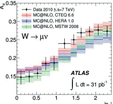
Figure 5.TheWcharge asymmetry in the muon decay channel,Aμ, measured by ATLAS as function
of the final state muon pseudorapidity|ημ|. The black
dots are ATLAS data, and the colored areas are different PDF predictions. From reference [8].
boson decays in proton-proton collisions, one can learn about the content of quarks and antiquarks inside the proton, i.e. about thestructureof the proton.
In theW path measurement, the students learn how to identify collision events where aW boson may have been produced (a “Wevent”) with a subsequent decay into a charged lepton and a neutrino. As mentioned before, such events will in general contain one charged lepton with a large momentum component in the plane perpendicular to the beam line and large missing transverse energy caused by the neutrino. This is exactly what the students need to look for to identifyW events. The students then count the number of identifiedW events where the final state charged lepton is positive (i.e. the number ofW+events), NW+, and the corresponding number of events where the charged lepton is negative,NW−. The final result of the analysis is the charge ratioNW+/NW−, a number which is sensitive to the structure of the proton.
Since the proton has two valence up quarks and only one valence down quark, a first naive ap-proximation to the charge ratio isNW+/NW− =2. The presence of sea quarks complicates the picture, and brings the charge ratio down to a value between 1 and 2.
As previously mentioned, the structure of the proton is summarized by the PDFs, so a charge ratio measurement can be used to test our knowledge of or constrain the PDFs of the proton. Such a measurement is an important physics result. The students doing theW path measurement are thus performing a measurement which is close to an actual important physics measurement performed by the ATLAS collaboration. A plot from the ATLAS analysis of theW charge asymmetry in the muon decay channel [8] is shown in figure 5. Instead of the charge ratio NW+/NW−, the closely
related charge asymmetryAμ=(NW+−NW−)/(NW++NW−) is presented as function of the final state
muon pseudorapidity1|η
μ|. The data are compared to different PDF predictions exactly because this
measurement is sensitive to the proton structure.
In theW path measurement, the students also look for events where two oppositely chargedW bosons may have been produced with subsequent decays into charged leptons and neutrinos. Such events are characterized by two oppositely charged final state leptons with large momentum compo-nents in the plane perpendicular to the beam line and large missing transverse energy caused by the
1The pseudorapidity is defined asη=−ln tan(θ/2) withθas the angle of a final state particle’s direction of motion with
two neutrinos. The production and decay of the Higgs boson may produce such a signature, as illus-trated in figure 3(b), and the students look at the distribution of the angle between the charged leptons in the plane perpendicular to the beam line to search for the Higgs boson. Further details on this, and on theWpath measurement in general, are given in reference [4].
5 The
Z
path and the invariant mass technique
TheZ path measurement deals with theinvariant masstechnique for particle identification and dis-covery, which will now be presented. As before mentioned, theW andZbosons are short lived, and decay in practice immediately after their creation. They can therefore only be observed via their decay products. The existence and properties of these and other short lived particles must be inferred from measurements of their decay products, and in this context, the invariant mass is a very useful concept. Consider a massive short lived particle decaying into several lighter particles. The energyEof the short lived particle is related to its momentumpand massmby
E2=p2c2+m2c4, (1)
wherecis the speed of light in vacuum. Assume now that the energies and momenta of the decay products are measured. Conservation of energy and momentum implies that
E=
i
Ei and p=
i
pi, (2)
where the sums run over the decay products andEi(pi) is the energy (momentum) of decay product numberi. Clearly, equation (1) can be solved for the massm, and inserting the relations (2), we obtain
m= 1 c4 ⎛ ⎜⎜⎜⎜⎜ ⎝ i Ei ⎞ ⎟⎟⎟⎟⎟ ⎠ 2 − 1 c2 ⎛ ⎜⎜⎜⎜⎜ ⎝ i pi ⎞ ⎟⎟⎟⎟⎟ ⎠ 2 . (3)
The expression on the right hand side is known as the invariant mass, and can be calculated for any set of measured final state particles. In the case that the final state particles are the decay products of a short lived particle, the invariant mass is equal to the mass of the short lived particle.
One can search for short lived particles by plotting distributions of invariant masses of final state particles in particle collisions such as the proton-proton collisions at the LHC. Short lived particles will give rise to peaks in such distributions. As an example, figure 6 shows the distribution of the invariant mass of opposite sign muon pairs,
Mμμ=
(Eμ++Eμ−)2
c4 −
(pμ++pμ−)2
c2 , (4)
Figure 6.The distribution of the invariant mass of opposite sign muon pairs,Mμμ, in a set of early LHC
collision data recorded by ATLAS. Each peak in this distribution corresponds to a particular short lived particle. The peak aroundMμμ=90 GeV/c2
corresponds to theZboson.
an invariant mass distribution would be the corresponding particle’s natural width, which is directly related to its lifetime.
The students doing theZpath measurement learn how to identify electrons and positrons, muons, and photons in the ATLAS detector. They look for events containing
• two oppositely charged leptons,
• two photons, or
• two pairs of oppositely charged leptons, i.e. four charged leptons in total.
The goal of the measurement is to produce invariant mass distributions and look for peaks corre-sponding to short lived particles. As in the case of theWpath, the analysis performed by the students follows closely the general procedure used in many important physics analyses performed by the ATLAS collaboration.
In the distribution of the invariant mass of pairs of oppositely charged leptons, the students may discover theZ boson as well as the J/ψandΥmesons. The peaks corresponding to these particles will be around 90 GeV/c2, 3 GeV/c2, and 10 GeV/c2respectively, and all of them are clearly visible in figure 6. In addition to these well known particles, the students may discover a new, heavier, version of theZ boson, called theZ. The latter is expected in theories involving hypothetical new interactions. Simulated events with the production and decay into leptons of this particle have been mixed in with the real data given to the students. This gives the students the possibility of really discovering something new and unexpected, and allows them to see how a new particle could be discovered at the LHC.
The distributions of the invariant mass of two photons and four charged leptons are in principle sensitive to the production and decay of the Higgs boson, as illustrated in figures 3(c) and 3(d). How-ever, the amount of data available for Masterclass use is not large enough for the students to actually see evidence of the Higgs boson. The inclusion of events with two photons and four charged leptons in theZ path measurement does, however, allow the students to learn about the Higgs discovery at
2In the axis label of figure 6,natural unitsare employed, so that mass, energy, and momentum all have the same physical
dimension. The unit GeV quoted on the horizontal axis of the plot corresponds to the mass unit GeV/c2. Natural units will be
the LHC. One should note that the data analyzed by the students contain real ATLAS Higgs candidate events.
6 The
Z
path Masterclass
When attending a standardZ path Masterclass event, the students spend one full day at their local university. The program begins in the morning with lectures on both theoretical and experimental aspects of particle physics. In the theoretical lectures, the particles and forces of the Standard Model are introduced. The experimental lecture introduces the invariant mass technique and explains how one can learn about short lived particles by studying their decay products. Furthermore, it deals with the experimental detection of particles using a particle detector. The structure of the ATLAS detector is introduced, and the students learn how different particles are “seen” in the detector.
After lunch, the students proceed with the actual practical measurement. Before they begin, there is a short demonstration where some key elements of the morning lectures are repeated. In particular, the procedures for identifying electrons and positrons, muons, and photons in ATLAS events are reviewed with some examples. The students then go to various computer rooms, where there is one computer available per two students. The students go together in groups of two, and proceed to analyze their own set of real LHC collision events recorded by ATLAS. Tutors are available for questions and guidance.
In the late afternoon, there is a results session. First, the results obtained by the students at the given university is discussed in a plenary session. Finally, the students take part in a video conference with all the other universities that participated in the International Masterclasses on the given day. The conference is led by moderators based at CERN. It includes discussion of the results obtained by all the universities, a quiz, and a question session where the students can ask the moderators about anything, for example what it is like to be a scientist and to be working at CERN.
6.1 The measurement
For the actual measurement, each group of two students is assigned a unique3 dataset containing 50 real LHC collision events recorded by ATLAS. The students analyze the events one by one by inspecting them visually in the event display program HYPATIA [9, 10]. For each event, the students should decide whether it could fall into one of the categories mentioned in section 5. If so, the students select the particles they believe to be electrons/positrons, muons, or photons, and HYPATIA calculates the invariant mass of the selected particles.
After the students have analyzed all their 50 events, a plain text file containing the calculated invariant masses is made. The students upload this file to the online plotting tool OPloT [11], where they can look at the invariant mass distributions they have obtained. The results uploaded to OPloT are used for combination plots shown in the afternoon results session at the university and in the video conference.
6.2 Event identification in HYPATIA
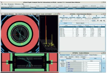
Figure 7 shows a screenshot of HYPATIA as it would appear to a student doing theZ path mea-surement. The lower left window shows two projections of the ATLAS detector, which are zoomed
3To the extent possible, every student group on a given day is assigned a unique dataset. If the number of participants on
Figure 7. A screenshot of the event display program HYPATIA as it would appear to a student doing theZ path measurement. This is a typical electron-positron event, with two pronounced clusters of energy deposits in the electromagnetic calorimeter and corresponding tracks in the tracking detectors. The measured charges corresponding to the two tracks can be checked in the “track momenta window” to the right to verify that the two electron/positron candidates are indeed oppositely charged. The dashed red line in the transverse projection gives the direction of the missing transverse energy, the magnitude of which is not particularly large in this event.
to show primarily the innermost parts of the detector in this particular example. In thetransverse projection (top), the beam line is perpendicular to the plane of the paper, while in thelongitudinal projection (bottom), the beam line is horizontal and in the plane of the paper. In the tracking detectors (grey), we see reconstructed tracks corresponding to the trajectories of charged particles. In the elec-tromagnetic (green) and hadronic (red) calorimeters, we see yellow dots corresponding to measured energy deposits. In this event, there are two pronounced clusters of energy deposits in the electro-magnetic calorimeter. Since there are also tracks in the tracking detector pointing in the direction of these clusters, we identify this event as an electron-positron event. The assumed electron and positron have been selected and inserted into the invariant mass window at the top. The invariant mass of the electron-positron pair in this event is 90.9 GeV/c2, so this is a typicalZboson event.
(a) (b)
Figure 8.HYPATIA event displays of a typical event with two muons (a) and a typical event with two photons (b). The muons are the only charged particles which pass through the whole detector and are detected in the muon spectrometer. The photons leave energy deposits in the electromagnetic calorimeter, but no tracks in the tracking detectors. Note that one of the photons is in the end-cap, and is therefore only seen in the longitudinal projection, as only calorimeter deposits from the barrel region are shown in the transverse projection.
A photon mayconvert into an electron-positron pair when interacting with the material of the tracking detector. In this case, there will be two tracks close together in the tracking detector pointing towards an energy cluster in the electromagnetic calorimeter. The students can calculate the invariant mass of the two tracks, which should be small if they are indeed the result of a converted photon.
6.3 The Oslo Plotting Tool (OPloT)
The Oslo Plotting Tool (OPloT) is the online plotting tool developed specifically for the analysis, combination, and presentation of results for theZ path Masterclass. When a group of students has finished analyzing their 50 events, they upload the resulting invariant mass file produced by HYPATIA to OPloT. Before uploading, the students must select their university and unique group number, so that each group of students upload to a unique file, and students do not overwrite each other’s data.
Immediately after uploading their file, the students can study their own results in the form of in-variant mass histograms. They can interactively change the inin-variant mass axis range, choose between linear and logarithmic binning, and set the number of bins. The distributions of the invariant mass of two charged leptons, two photons, and four charged leptons can be viewed individually and together. Figure 9 shows the two lepton4 invariant mass distribution obtained by a particular group of stu-dents in theZ path Masterclass on the 15th of March 2013. The figure shows the distribution as presented by OPloT with a logarithmic invariant mass axis. With the 50 event dataset analyzed by
4The terms “two lepton”, “two photon”, and “four lepton” are here used to label the events with a pair of oppositely
Figure 9. The two lepton invariant mass distribution obtained by a particular group of students in theZpath Masterclass on the 15th of March 2013. The figure shows the distribution as presented by OPloT with a loga-rithmic invariant mass axis. Thee+e−andμ+μ−contributions are shown in different colors. The average values and sample standard deviations of the invariant mass values within four mass regions are presented in the table to the right of the plot. The boundaries of the mass regions can be set by the students, and correspond here to windows around theJ/ψ,Υ,Z0, andZmasses. The average invariant mass value can be taken as an estimate of the relevant particle’s mass, and the sample standard deviation as a measure of the width of the peak. The width of the peak is related to the particle’s lifetime and the experimental resolution.
these students, it is already clear that theZboson is observed beyond doubt, with more than 20 events in the two bins around 90 GeV/c2. There is also a bin with several events around 10 GeV/c2, and two exciting events around 1 TeV/c2. Finally there seems to be a hint of something around 40 GeV/c2, but this is a fluctuation which will be seen to wash out when combining with the results of other students. Figure 10 shows the four lepton and two photon invariant mass distributions obtained by the same group of students. The three observed four lepton events is consistent with the expectation for a 50 event sample, and the event close to 125 GeV/c2 may indeed be one of the prime Higgs candidate events observed by ATLAS. The students have also identified a few two photon events, but not as many as expected in a 50 event sample.
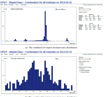
OPloT can make invariant mass distributions where the data from many students are combined. In particular, one can choose to combine all the student data from a given university on a given day, or all the student data from all universities taking part in the International Masterclasses on a given day. The former combination is used for the plenary discussion of results locally at each university, while the latter combination is used when results are discussed in the video conference at the end of the day. Figure 11 shows the invariant mass distributions resulting from the combination of all submitted results from all universities taking part in the International Masterclasses on the 15th of March 2013. The two lepton invariant mass distribution in figure 11(a) shows clear evidence of the J/ψandΥ mesons as well as theZ boson. It is also clear that the students have discovered a new particle with a mass of 1 TeV/c2. Although this is because of the simulated events mixed in with the real data as mentioned earlier, it allows the students to see what the discovery of a new particle may look like. Ob-viously, it is explained to the students during the results session that the peak at 1 TeV/c2is due to the simulated events. We also observe a smooth “continuum” distribution between the peaks. This must be coming primarily from misidentification by the students, as no two lepton events with invariant masses outside the peak regions were mixed into the event samples for the 2013 Masterclasses. It is interesting to note that electron-positron events dominate completely the regions between the peaks, as expected from the fact that an electron-like experimental signature is rather easily mimicked by hadrons, of which there are always plenty in proton-proton collision events.
The four lepton invariant mass distribution in figure 11(b) shows that the students are very eager to look for such events, and possibly that they should be more critical in their particle identification. In fact, only around 30 four lepton events were selected and mixed into the event samples5 for the 2013 Masterclasses, while the students have identified more than 300.
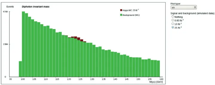
A couple of things can be noted also about the two photon invariant mass distribution in fig-ure 11(c). There is clearly a peak around 90 GeV/c2, and since theZ boson can not decay into two photons, this peak must be coming from the misidentification of electrons as photons by the students. Above 100 GeV/c2, the distribution looks pretty much as expected, but the statistical fluctuations are clearly too large for a small peak due to the Higgs boson to be discovered. It is important that the students understand that this is a limitation of the size of the data sample, and that the two photon invariant mass distribution was in fact a key ingredient in the Higgs discovery at the LHC. This is discussed in the plenary results session and the video conference, and to aid the discussion, one can in OPloT choose to display simulated data corresponding to different data sample sizes in order to show how a Higgs peak becomes more apparent as the amount of data increases. The simulated data corresponding to a large data sample (25 fb−1of integrated luminosity, which can be compared to the approximate 1 fb−1 available to the students6) is shown in figure 12. Here, it should be possible to
5The aforementioned intentional duplication of four lepton events is handled by OPloT, and is not responsible for the large
number of such events compared to the expectation.
6In the students’ data, about 25 Higgs events are expected in the two photon invariant mass distribution. In the four lepton
(a) The combined two lepton invariant mass distribution.
(b) The combined four lepton invariant mass distribution.
(c) The combined two photon invariant mass distribution.
Figure 12.The two photon invariant mass distribution presented by OPloT when set to display simulated back-ground and Higgs signal corresponding to an integrated luminosity of 25 fb−1.
convince oneself that the peak due to the Higgs boson would be visible even if it were the same color as the background.
Even though examples are not shown here, there are further interesting possibilities in OPloT for the two photon invariant mass distribution. One can choose to compare the students’ distribution to simulated background and signal distributions corresponding to the size of the data sample available to the students. If all the available data have been analyzed by the students, and the students have done a good job with the event identification, it should be possible to observe good agreement between the student data and the simulated data. Finally, the student data can be replaced by the “correct” distribution, resulting from the selection of events using ATLAS software analysis procedures.
Also in the four lepton invariant mass distribution, one can choose to display simulated Higgs signal in OPloT. One can then see the expected size of a Higgs signal in this distribution, and discuss in the plenary session and video conference how it could be used to discover the Higgs boson. The students should understand that also the four lepton invariant mass distribution was a key ingredient in the Higgs discovery at the LHC, but that it looks very different from the two photon distribution, as the expected numbers of background and signal events are both much smaller in the four lepton distribution.
7 Summary and outlook
The physics behind the ATLASW andZpath Masterclass measurements has been presented. While theW path measurement deals with both the structure of the proton and the search for the Higgs boson, theZpath measurement is devoted completely to searches for short lived particles.
TheZpath measurement has been presented in more detail. We have seen how the students iden-tify final state particles in the event display program HYPATIA, and how their results are presented in the online plotting tool OPloT. The interpretation of the results in terms of short lived particles has been reviewed, and while evidence of the Higgs boson could not be observed in the students’ distri-butions, the two photon and four lepton invariant mass distributions were both discussed in terms of the Higgs search at the LHC.
in theZpath Masterclass, the students could possibly discover the Higgs boson themselves. In case other new particles are discovered at the LHC, theZpath measurement can be updated to allow the students to discover these particles as well. In this way, the measurement can be kept “fresh” and closely related to the latest LHC results.
References
[1] U. Bilow and M. Kobel,International Masterclasses – Bringing LHC Data to School Children, these proceedings
[2] International Masterclasses, http://physicsmasterclasses.org/
[3] International Particle Physics Outreach Group (IPPOG), http://ippog.web.cern.ch/
[4] U. Bilow, C. Hasterok, K. Jende, M. Kobel, C. Rudolph, and J. Woithe,ATLAS W Path – real data from the LHC for high school students, these proceedings
[5] G. Aad et al. (ATLAS collaboration), Phys. Lett. B716, 1-29 (2012) [6] S. Chatrchyan et al. (CMS collaboration), Phys. Lett. B716, 30 (2012) [7] A. Martin, W. Stirling, R. Thorne, and G. Watt, Eur. Phys. J. C63, 189 (2009) [8] G. Aad et al. (ATLAS collaboration), Phys. Lett. B701, 31-49 (2011)
[9] S. Vourakis,Bringing high energy physics to the classroom with HY.P.A.T.I.A., these proceedings [10] Ch. Kourkoumelis, D. Fassouliotis, S. Vourakis, and D. Vudragovic, HYPATIA, http://hypatia.
phys.uoa.gr/