Evaluation of Sequence Learning Models for Large
Commercial Building Load Forecasting
Cristina Nichiforov1 , Grigore Stamatescu1,2 , Iulia Stamatescu1 , Ioana F˘ag˘ar˘a¸san1
1 Department of Automatic Control and Industrial Informatics, Faculty of Automatic Control and Computers,
University Politehnica of Bucharest, 313 Splaiul Independentei, 06004 Bucharest, Romania;
1
2
3
4
5
6
7
8
9
10
11
12
13
14
15
16
[email protected] (C.N.); [email protected] (I.S.); [email protected] (I.F.)
2 Institute of Technical Informatics, Technical University of Graz, 16 Inffeldgasse, 8010 Graz, Austria;
* Correspondence: [email protected]; Tel.: +40-723-425-323
Abstract: Buildingshave startedto playacritical rolein the stabilityandresilience of modern
smartgrids,leadingtoarefocusingoflargescaleenergymanagementstrategiesfromthesupply
sideto the consumer side. When the buildingsintegrate localrenewableenergy generation in
theformofrenewableenergyresourcestheybecomeprosumersandthisreflectsintoadditional
complexityintotheoperationoftheinterconnectedcomplexenergysystems. Aclassofmethods
ofmodellingtheenergyconsumptionpatternsofthebuildinghaverecentlyemergedasblack-box
input-outputapproacheswiththeabilitytocaptureunderlyingconsumptiontrends.Thesemakeuse
andrequirelargequantitiesofqualitydataproducesbynon-deterministicprocessesunderlyingthe
energyconsumption.Wepresentanapplicationofaclassofneuralnetworks,namelydeeplearning
techniquesfortimeseriessequencemodellingwiththegoalofaccurateandreliablebuildingenergy
loadforecasting. TheRecurrentNeuralNetworkimplementationusesLongShort-TermMemory
layersinincreasingdensityofnodestoquantifypredictionaccuracy.Thecasestudyisillustrated
onfouruniversitybuildingsfromtemperateclimatesoveroneyearofoperationusingareference
benchmarkingdatasetthatallowsreplicableresults.Theobtainedresultsarediscussedintermsof
accuracymetricsandcomputationalandnetworkarchitectureaspectsandareconsideredsuitablefor
furtherusedinfutureinsituenergymanagementatthebuildingandneighbourhoodlevels.
Keywords:sequencemodels;recurrentneuralnetworks;energymodelling;smartbuildings. 17
1. Introduction 18
Complex energy systems which support global urbanisation tendencies are playing an important 19
role in the definition, implementation and evaluation of future smart cities. Within the built 20
environment, making use of modern technologies in the areas of sensing, computing, communication 21
and control leads to an improvement the operations of various systems and the well-being of its 22
inhabitants. Of particular relevance to the reliable, clean and cost-effective energy supply electrical 23
grid, thereby assuring a to ever increasing urban needs. The main target of our work is developing 24
improved models for load forecasting of medium and large commercial buildings which act in a 25
determining role as consumers, prosumers or balancing entities for grid stability. Statistical learning 26
algorithms such as classical and deep neural networks represents a prime example. Black-box model 27
achieved thorough such techniques have proven able to accurately model underlying patterns and 28
trends driving energy consumption can be used to forecast load profiles and improve high level control 29
strategies. In such way significant economic, through cost savings, and environmental, through limited 30
use of scarce energy resources, benefits can be achieved. 31
An often quoted figure in the scientific literature [1] places the building energy use at almost 40% 32
of primary energy use in many developed countries with an increasing trend. In modern buildings 33
a centralised software solution, often denoted as a Building Management System (BMS), collects all 34
the relevant data streams originating in the building subsystems and provides means for intelligent 35
algorithms to act based on the processed data. Energy-relevant data, generated through heterogeneous 36
instrumentation networks is subsequently leveraged to control relevant energy parameters in daily 37
operation. For the existing older building, new technology can be used to upgrade legacy devices 38
such as electrical meters and integrate them into wired or wireless communication networks, in a cost 39
effective manner. Finally the resulting preprocessed energy measurements time series serve as input 40
for accurate models of energy prediction and control. 41
Statistical learning algorithms have become robust and well-adopted in the last years through 42
concentrated efforts in both research and industry. This was stimulated by data availability and 43
exponentially increasing computing resources at lower costs, including cloud systems. Neural 44
networks are one example of such algorithm which offers good results in many application areas, 45
including modelling and prediction of energy systems. This is valid for both classification tasks, as 46
well as regression tasks where the objective is to predict an output numerical value of interest. Deep 47
learning networks are highly intricate neural networks with many hidden layers that are able to 48
learn patterns of increasing complexity in input data sets. Initially deployed through industry driven 49
initiatives in the areas of multimedia processing and translation systems, other technical applications 50
currently stand to benefit from the availability of open-source algorithms and tools. For time series 51
and sensor data, a particular types is gaining adoption with the research community namely sequence 52
models based on recurrent neural network that can capture long term dependencies in input examples. 53
In the nomenclature described by [2] of machine learning (ML) taxonomy for smart buildings, our work 54
fits within the area of using ML to estimate aspects related to either energy or devices, in particular 55
energy profiling and demand estimation. 56
Within this approach, large commercial buildings provide the operators/owners with the 57
economic incentives and return of investment related to energy efficiency projects where small 58
percentage gains on large absolute values of energy use become more attractive. An equally large 59
market exist for improving energy forecasting accuracy in the residential sector, which is however 60
more fragmented and the incentives to deploy such approaches have to be present at the energy 61
supplier or through public large scale programs. 62
Main contributions of the paper can be thus summarised: 63
• illustrating a deep learning approach to model large commercial building electrical energy usage
64
as alternative to conventional modelling techniques; 65
• presenting an experimental case study using the chosen deep learning techniques enabling
66
reliable forecasting of building energy use; 67
• analysis of the results in terms of accuracy metrics, both absolute and relative which provide a
68
way for replicable results towards other related research. 69
Additional contributions which extend the previous conference paper [3] are summarised. We 70
have provided, as main goal for the extended version, new experimental results for recurrent neural 71
network modelling of large commercial building energy consumption. These are further analysed 72
also taking into account several performance metrics and computational aspects. More technical 73
clarifications regarding the methods and data processing and modelling pipeline are also included. 74
Also, significant revisions and extensions have been carried out to the related work section for a more 75
timely and focused state-of-the-art to frame the work as well as to other parts of the paper to improve 76
readability and allow the replication of the results by interested researchers on the neural network 77
architectures presented in an energy management system. 78
The rest of the paper is structured as follows. Section II discusses timely related work for energy 79
consumption modelling of direct relevance to the previously stated contribution areas. Section III 80
presents the theoretical background of Recurrent Neural Networks (RNN) implemented with layers of 81
Long Short-Term Memory (LSTM) units and their application for this task. A case study is described 82
in Section IV by applying the deep learning techniques on a reference benchmarking dataset for four 83
aspects pertaining to the architectures of the learning algorithms that were implemented. Section V 85
concludes the paper with regard to applicability of the derived black-box models for in situ electrical 86
load forecasting. 87
2. Related Work 88
We first state three key factors identified as drivers of the application of statistical learning 89
techniques and algorithms to energy system modelling and control: 90
• better availability of good quality datasets and computational resources that enable extensive
91
testing and validation of the proposed methods; 92
• commercial and open-source algorithm libraries and software with suitable documentation and
93
examples for a wider audience; 94
• increased collaboration between algorithm, computing and control experts and domain
95
specialists in the energy and civil engineering fields; this has influenced the design of new 96
deep learning architectures customised mostly for particular applications. 97
[4] describe an approach and case study for prediction of household energy consumption using 98
feed-forward back propagation neural networks. The authors discuss their outcomes based on data 99
collected from four residential buildings in South Korea, including the preprocessing and tuning 100
of the algorithms. The evaluation is based on models built on raw data, normalised data and data 101
with statistical moments with the conclusion that the accuracy metrics are best in the latter case. 102
Learning customer behaviours for effective load forecasting is discussed by [5] who implement Sparse 103
Continuous Conditional Random Fields (sCCRF) to effectively identify different customer behaviours 104
through learning. A hierarchical clustering process is subsequently used to aggregate customers 105
according to the identified behaviours. 106
In [6] the authors focus on two deep learning techniques for building energy consumption namely 107
Conditional Restricted Boltzmann Machines (CRBM) and Factored Conditional Restricted Boltzmann 108
Machines (FCRBM). The results are illustrated in comparison to artificial neural networks and support 109
vector machines (SVM) as well as recurrent neural networks. It is shown that for many of the test 110
scenarios: aggregated and submetering data as well as different time horizons and resolution, the 111
investigated methods offer better performance in terms of RMSE on the prediction horizon. Time series 112
change point detection along with preprocessing approaches are introduced in [7]. SEP algorithm is 113
evaluated on smart home data, both real and artificial. This uses separation distance as a divergence 114
measure to detect change points in high-dimensional time series. Building occupancy influence on 115
energy consumption through indirect sensing is elaborated upon by [8] where the system is able to 116
infer occupancy counts using "proxy" measures of temperature and indoor CO2 concentrations. 117
The authors of [9] present an end-to-end deep learning approach for load forecasting of 118
commercial buildings by combining stacked autoencoders (SAE) with extreme learning machines 119
(ELM). SAE extracts the relevant features from the input dataset while ELM works as the predictor. 120
The advantages of this particular method are justified in terms of achieving directly the output weights 121
of the networks without iterative backpropagation. Two RNN models based on LSTM units for 122
building energy consumption are evaluated in [10]. An important finding of this study is that RNN 123
methods tend to perform better than others when applied to aggregated energy data and long term 124
dependencies are more difficult to identify. Also the authors use the resulting model to perform 125
missing value imputation on the original time series. [11] discuss the application of auto-encoders 126
and generative networks as deep learning alternative to conventional feature engineering in learning 127
models for electrical energy load forecasting. A method based on Support Vector Regression (SVR) is 128
presented by [12]. 129
While defining the context of the current work, we mention also previous implementation 130
which analysed conventional system identification using Auto-Regressive Integrated Moving Average 131
have been tested [14] in terms of number of hidden layers and number of neurons per layer. The deep 133
learning approach offers better results for our test scenarios. The final aim is to integrate the resulting 134
validated models in a building energy decision support system, in a similar fashion to [15]. 135
3. Electrical Load Forecasting using Sequence Model Recurrent Neural Networks 136
Recurrent neural networks (RNN) are becoming a very important modelling tool in applications 137
where the input data consists of time-related sequences of "events". The inherent loop presents in an 138
RNN carry long-term dependencies toward the final outcome. By simultaneously processing multiple 139
elements in a sequence of inputs they are directly applicable for the evaluation of non-linear time 140
series problems, such as electrical energy load forecasting. Given the differences to conventional 141
artificial neural networks (ANN), RNNs use back-propagation through time (BPTT) [16] or real-time 142
recurrent learning (RTRL) [17] algorithms to compute the gradient descent after each iteration for 143
solving the optimisation problem. As summary, RNNs are a type of artificial neural network that 144
include additional weights to the network to create cycles into the network graph in order to control 145
the internal state of the network. 146
3.1. RNN Implementation with LSTM 147
Recurrent neural network can be implemented using typical with sigmoid, tanh and rectifier 148
linear unit activation functions or by more advanced units which help better manage the information 149
flow throughout the network. Of the latter category, most popular currently with researchers are 150
Gated Recurrent Units (GRU) and Long Short-Term Memory (LSTM) units. The main purpose of 151
such techniques is to mitigate the effect of vanishing or exploding gradients during the training with 152
long sequences of input data which creates significant numerical computation problems during the 153
optimisation steps. The LSTM [18] structure contributes to enhance gradient flow over long sequences 154
during training by means of self-connected "gates" in the hidden units. In a LSTM network the flow of 155
information through the network is handled by reading, writing and removing information from the 156
memory [19,20]. 157
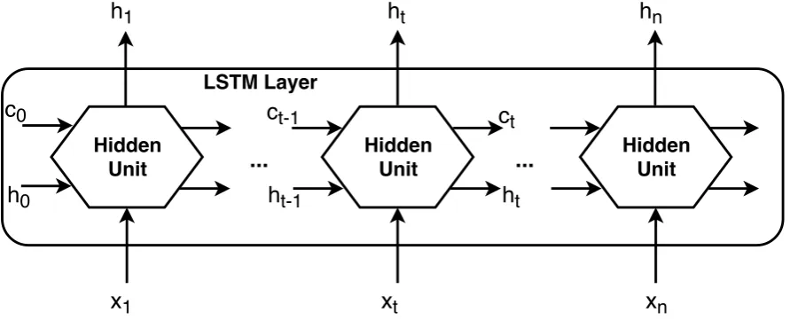
Figure1illustrates the flow of a time seriesxof lengthn, (n∈N) through an LSTM layer. In this
158
diagram,hstands for output, also hidden state, andcstands for cell state. The first LSTM hidden unit
159
takes the initial state of the network, (c0,h0) and also the first time step of the sequencex1and after
160
that computes the first outputh1and the updated cell statec1. This process repeats every time step.
161
LSTM Layer
Hidden
Unit
Hidden
Unit
Hidden
Unit
...
...
h
1h
th
nx
1x
tx
nh
t-1h
th
0c
0c
t-1c
t
Figure 1.LSTM layer diagram
The state of the LSTM layer consists of the output state(h)and the cell state(c). On the one hand,
162
the output state at time steptcontains the output of the LSTM layer for this time step, and on the other
163
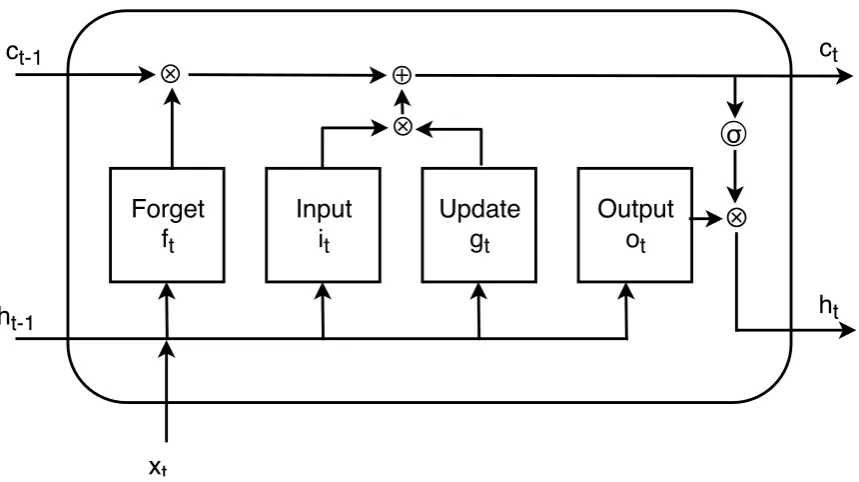
layer writes information to the cell state or erases information from it, where the layer controls these 165
updates using "gates". The "gates" represent components that control the cell state and the output state 166
of the layer. There are four such components: the input gate(i)which controls the level of cell state
167
update, the layer input(g)which adds information to cell state, the forget gate(f)which controls the
168
level of cell state reset and the output gate(o)which controls the level of cell state added to output
169
state [20]. 170
The diagram in Figure2illustrates the data flow at a specific time steptinside of a hidden unit.
171
Forget
f
tInput
i
tUpdate
g
tOutput
o
tσ
c
t-1h
t-1c
th
t⊕
⊗
⊗
⊗
x
tFigure 2.LSTM hidden unit diagram
A LSTM layer has the following learnable parameters: the input weights(W), the recurrent
weights(R)and the bias(b). W,Randbrepresents matrices that consists of concatenations of the
input weights, recurrent weights, and the bias of each component. The structure of each matrix is the following:
W=
Wi
Wf
Wg
Wo
,R=
Ri
Rf
Rg
Ro
,b=
bi
bf
bg
bo
,
wherei,f,gandorepresent the input gate, forget gate, layer input and output gate, respectively.
172
The state of the cell memory at time steptis updated recursively using the following formula
173 [18]: 174
ct= ft⊗ct−1⊕it⊗gt, (1)
where⊗stands for Hadamard product and the formulas for every component at time steptare:
ft=σ(Wfxt+Rfht−1+bf),
it=σ(Wixt+Riht−1+bi),
gt=tanh(Wgxt+Rght−1+bg),
(2)
σstands for the sigmoid function and tanh for hyperbolic tangent function.
175
The output state at time steptis given by the output gate(o)which implements a read function
176
combined with the cell state(c). The process is described by the following formula:
ht=ot⊗tanh(ct), (3)
where
ot=σ(Woxt+Roht−1+bo). (4)
A simplified version of LSTM has been introduced by [21] named Gated Recurrent Unit (GRU). In 178
this case the RNN cell uses a sole update gate and merges the cell and output states into a single value 179
that is propagated across the network. A recent application of GRU vs. LSTM in electrical energy load 180
forecasting is provided by [22]. 181
3.2. Benchmarking data sets 182
We leverage and acknowledge the data sets within the Building Data Genome at the the 183
Building and Urban Data Science (BUDS) Group at the National University of Singapore -184
http://www.budslab.org. This includes active power load traces and are part of a data collection of
185
several hundreds of non-residential buildings, mainly academic venue, proposed for performance 186
analysis and algorithm benchmarking to a common baseline [14,23]. 187
The current study investigates a RNN LSTM modelling approach through using various neural 188
network configurations and the assessment of performance between all forecasting LSTM models. 189
Key joint characteristics of the benchmarking data sets is the sampling period of the measurement 190
of 60 minutes over a 1-year period. We select four educational buildings with an approximate 191
surface area of 9.000 square meters. The chosen buildings for the study are from university campuses 192
in Chicago (USA), two reference buildings, New York (USA) and Zurich (Europe). After the 193
pre-processing of the noise and missing data in the initial data set using the median filter technique 194
two time series data sets were obtained with approximately 8.670 data points each. The median filter 195
[24] is expressed as: 196
y(n) =med[x(n−k),x(n−k+1), ...,x(n), ...,x(n+k−1),x(n+k)] (5)
wherey(n)is the filtered output of thex(n)input sequence. The sole parameter used for tuning the
197
filter is represented by the filter lengthn=2k+1. In our case, a 15th order median filter is used by the
198
preprocessing implementation. 199
The key criteria for the selection were: medium to large building, mixed usage pattern - office, 200
laboratory space, some classrooms and non-extreme temperate climate with four distinct seasons [14]. 201
A guiding choice in selecting the four candidates from the 508 entities in the dataset has been also 202
similarity to a local university building from our campus where a data collection study is currently 203
ongoing. 204
4. Experimental Evaluation for Building Energy Time-Series Forecasting 205
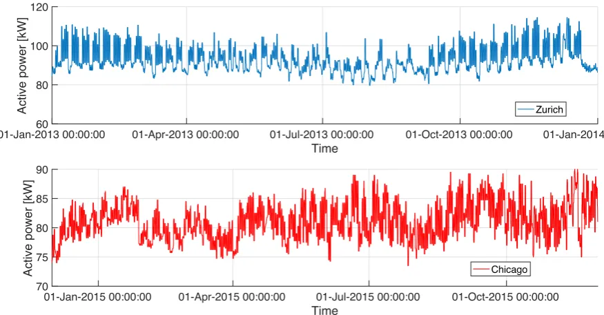
We present first the preprocessed time series for the buildings that make up our study and consist 206
of hourly active power measurement from the electrical meters. Figure3presents the input data for the
207
buildings in Zurich and Chicago, while Figure4presents the input data for the buildings in New York
208
and the second Chicago building. All are from academic campuses and in terms of absolute electrical 209
energy load, New York uses the most energy, followed by Zurich and Chicago in a similar range, and 210
with Chicago 2 having the least energy needs. 211
The classical LSTM algorithm was implemented for experimental assessment and forecasting. 212
The base network architecture consists of one sequence input layer, one hidden LSTM layer of varying 213
unit numbers, one fully connected layer and one regression output layer for the resulting forecasted 214
output value. Each network has a different configuration represented by the number of the hidden 215
units from the LSTM layer. Based on this, the following network structures were implemented, in 216
01-Jan-2013 00:00:00 01-Apr-2013 00:00:00 01-Jul-2013 00:00:00 01-Oct-2013 00:00:00 01-Jan-2014 00:00:00
Time
60 80 100 120
Active power [kW] Zurich
01-Jan-2015 00:00:00 01-Apr-2015 00:00:00 01-Jul-2015 00:00:00 01-Oct-2015 00:00:00
Time
70 75 80 85 90
Active power [kW] Chicago
Figure 3.Data sets used for LSTM estimation and testing: Zurich and Chicago buildings
Z-4, C2-0, C2-1, C2-2, C2-3, C2-4, NY-0, NY-1, NY-2, NY-3, NY-4. In our case the identifier before the 218
dash sign reflects the analysed building: Cstands for the Chicago building,Zfor the Zurich one,
219
C2 for the second building from Chicago andNYfor the New York building. The number after the 220
building identifier marks the complexity of the network in terms of hidden units of LSTM that were 221
implemented in the hidden layer, using a linear increase. This ranges from 5 hidden units for id 0, 25 222
hidden units for id 1, 50 hidden units for id 2, 100 hidden units for id 3 and finally 125 hidden units for 223
id 4. 224
The optimisation method of choice for training the neural networks was through the Adaptive 225
Moment Estimation (ADAM) algorithm [25]. This is an often used general optimisation method for first 226
order gradient based optimisation of stochastic objective functions with momentum. The algorithm 227
computes learning rates that can adapt in a automatic manner to the loss function which is optimised, 228
for each parameter from estimates of first and second moments of the gradients. It maintains an 229
element-wise moving average of the parameter gradients and their squared values, respectively . In 230
the literature is demonstrated that the algorithm is efficient in terms of computational time, has little 231
memory requirements and is suitable for large data problems. 232
One of the key optimisation parameters for carrying out the neural network training is the learning 233
rate. This allows implementing a trade-off between the speed of the processing and its precision, in 234
the sense that a large learning rate can in many situation miss the optimal value of the objective metric. 235
In our case the learning rate was established through an empirical adjustment process. The initial 236
value was set at 0.1 followed by subsequent decreases with a factor of 0.2 every 200 iterations. From 237
observing the performance over multiple initial training runs, a second parameters, the number of 238
training iterations, was set at 200. 239
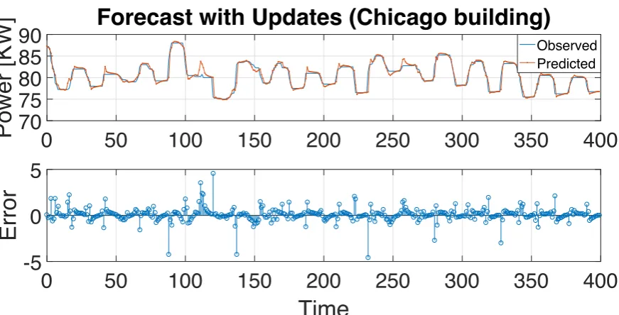
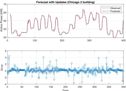
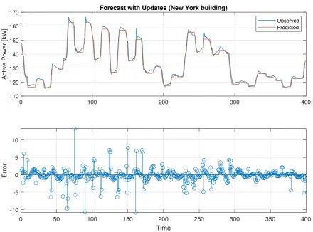
Figure5,6,7and8presents the prediction response by the LSTM neural network with 50 hidden
240
units in the LSTM layer versus real data for Chicago building and Zurich building, respectively. The 241
plots demonstrate that the forecasting performances of the LSTM models for the testing data sets is 242
very good. 243
01-Jul-2014 00:00:00 01-Oct-2014 00:00:00 01-Jan-2015 00:00:00 01-Apr-2015 00:00:00 40
50 60 70 80 90
Active Power [kW]
Chicago 2
01-Jan-2015 00:00:00 01-Apr-2015 00:00:00 01-Jul-2015 00:00:00 01-Oct-2015 00:00:00 01-Jan-2016 00:00:00
Time
80 100 120 140 160 180
Active Power [kW]
New York
Figure 4.Data sets used for LSTM estimation and testing: Chicago 2 and New York buildings
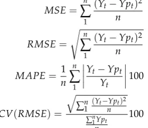
have included the Coefficient of Variation of the Root Mean Square Error CV(RMSE) based on the evaluation discussed in [11]. The metrics are computed according to the following equations:
MSE=
n
∑
1
(Yt−Ypt)2
n
RMSE=
sn
∑
1
(Yt−Ypt)2
n
MAPE= 1
n
n
∑
1
Yt−Ypt
Yt
100
CV(RMSE) = q
∑n
1
(Yt−Ypt)2
n
∑n 1Ypt
n
100
(6)
wherenrepresents the number of samples,YtandYptstand for the actual data and predicted data,
244
respectively. 245
A summary of the experimental results is listed in Tables 1-4 show These include: the error metrics 246
MSE, RMSE, CV (RMSE) and MAPE as well as training/computation time for the previously defined 247
RNN LSTM networks. 248
Table 1.Summary of accuracy metrics for RNN LSTM model forecasting: Chicago
C-0 C-1 C-2 C-3 C-4
Time(s) 75 93 143 247 330
MSE 0.6295 0.6132 0.5553 0.7486 0.9555 RMSE 0.7934 0.7831 0.7452 0.8652 0.9775 CV(RMSE)(%) 0.98 0.97 0.92 1.07 1.2 MAPE(%) 0.5623 0.5091 0.4945 0.5535 0.8177
The main outcome of the learning models, as reflected by the aggregate performance metrics from 249
Table1,2,3and4pinpoint the best network architecture for all four testing scenarios to be the one
250
with 50 LSTM units in the hidden layer. Also, Figure9presents the evolution of the MAPE error and
0
50
100
150
200
250
300
350
400
70
75
80
85
90
Power [KW]
Forecast with Updates (Chicago building)
Observed Predicted-5
0
5
Error
0
50
100
150
200
250
300
350
400
Time
Figure 5.Building Load Forecasting with 50 unit RNN LSTM: Chicago
0
50
100
150
200
250
300
350
400
80
90
100
110
120
Power [KW]
Forecast with Updates (Zurich building)
Observed Predicted
-10
0
10
Error
0
50
100
150
200
250
300
350
400
Time
Figure 6.Building Load Forecasting with 50 unit RNN LSTM: Zurich
Table 2.Summary of accuracy metrics for RNN LSTM model forecasting: Zurich
Z-0 Z-1 Z-2 Z-3 Z-4
Time(s) 76 94 150 275 355
MSE 2.3846 2.1732 2.0506 2.2506 2.034 RMSE 1.5442 1.4742 1.432 1.5002 1.5107 CV(RMSE)(%) 1.66 1.59 1.58 1.61 1.63 MAPE(%) 0.9197 0.9008 0.828 0.9958 3.4684
computation time for each building over each defined network. It can be seen that the computation 252
time increases quite linearly with the number of the neurons in the LSTM layers which can be helpful 253
for deploying more tests. We can affirm that until we achieve the best value for MAPE error, 50 neurons 254
in the LSTM layer, this is a good compromise, but after this point the computation time increases too 255
much without any better performances. The reference computer includes a 2.6 GHz 7th generation 256
Intel i5 CPU, 8GB of RAM and a solid state disk, with Windows 10 as operating system. This is the 257
0 100 200 300 400 50
55 60 65 70
Active Power [
k
W]
Forecast with Updates (Chicago 2 building)
Observed Predicted
-4 -2 0 2 4 6
Error
0 50 100 150 200 250 300 350 400
Time
Figure 7.Building Load Forecasting with 50 unit RNN LSTM: Chicago 2
Table 3.Summary of accuracy metrics for RNN LSTM model forecasting: Chicago 2
C2-0 C2-1 C2-2 C2-3 C2-4
Time(s) 72 91 137 280 347
MSE 0.8013 0.7801 0.7163 0.7626 0.8413 RMSE 0.8952 0.8832 0.8464 0.8733 0.9172 CV(RMSE)(%) 1.63 1.6 1.53 1.57 1.65 MAPE(%) 1.0005 0.9439 0.8982 0.9736 1.019
Table 4.Summary of accuracy metrics for RNN LSTM model forecasting: New York
NY-0 NY-1 NY-2 NY-3 NY-4
Time(s) 79 102 145 294 346
MSE 5.4433 5.4012 4.7778 5.1203 5.5522 RMSE 2.3309 2.3241 2.1858 2.2628 2.3563 CV(RMSE)(%) 1.75 1.73 1.7 1.72 1.78 MAPE(%) 1.0409 1.004 0.9602 0.9813 1.1073
and run under MATLAB, version R2018a, which provides a robust high-level technical programming 259
environment. We leverage built-in functions from the machine and deep learning toolboxes as well as 260
dedicated scripts for data ingestion and preprocessing. 261
Table5provides a summary of the statistical indicators for the comparable relative accuracy
262
metrics: CV-RMSE and MAPE over the tested scenarios, four building with five networks each. The 263
reported statistical indicators are: minimum, maximum, meanµ, standard deviationσ, skewness and
264
kurtosis. 265
The performance evolution during training for the Zurich and New York buildings is graphically 266
0 100 200 300 400 110
120 130 140 150 160 170
Active Power [kW]
Forecast with Updates (New York building)
Observed Predicted
-10 -5 0 5 10
Error
0 50 100 150 200 250 300 350 400
Time
Figure 8.Building Load Forecasting with 50 unit RNN LSTM: New York
Table 5.Statistical indicators for relative peformance metrics CV-RMSE and MAPE
Min Max µ σ s k
CV (RMSE) 0.92 1.78 1.4935 0.2873 −1.0846 2.5502 MAPE 0.4945 3.4684 0.9989 0.6108 3.4661 14.8790
200 iterations, with the worst and best case scenarios. In the first case the worst performance is seen 268
on the Z4 network which tries to overfit the data given the more complex structure and as such the 269
RMSE presents multiple increases and decreases over the training horizon. In the positive case, Z2, we 270
observe convergence in just under 100 training iterations as compared to the previous 120 iterations 271
needed by the denser network. Similar networks are represented for the New York dataset. A different 272
behaviour is observed in this case with where the best-case convergence of the RMSE is slower at the 273
beginning with a more gentle slope of the graphic over the first steps. 274
5. Conclusions 275
We have presented an application of sequence models, implemented by means of Recurrent 276
Neural Network with Long Short-Term Memory units, for electrical energy load forecasting in large 277
commercial buildings. Results have shown good performance for modelling and forecasting accuracy 278
while evaluating against typical time series based metrics such as: MSE, RMSE, CV-RMSE and 279
MAPE. Generally, based on the number of layers that were selected, a value around 50 LSTM units 280
in the hidden layer was found to yield the best estimates for the underlying time series. Beyond 281
this the network has a strong tendency to overfit the input data and perform poorly on the testing 282
samples. The results have been evaluated on year-long selected building energy traces from a reference 283
C-0 C-1 C-2 C-3 C-4 0 0.5 1 MAPE[%] Chicago Building 0 200 400 MAPE error MIN(MAPE) Time[s]
Z-0 Z-1 Z-2 Z-3 Z-4
0.5 1 1.5 2 2.5 3 3.5
4 Zurich Building
50 100 150 200 250 300 350 400 MAPE error MIN(MAPE) Time[s]
C2-0 C2-1 C2-2 C2-3 C2-4
Network 0.88 0.9 0.92 0.94 0.96 0.98 1 1.02 MAPE[%]
Chicago 2 Building
50 100 150 200 250 300 350 MAPE error MIN(MAPE) Time[s]
NY-0 NY-1 NY-2 NY-3 NY-4
Network 0.95
1 1.05 1.1
1.15 New York Building
0 100 200 300 400 MAPE error MIN(MAPE) Time[s]
Figure 9.Computation Time vs. MAPE Error evolution for each building
Training Progress (05-Jun-2018 13:35:34)
0 20 40 60 80 100 120 140 160 180 200
Iteration 0 1 2 3 4 5 6 7 RMSE 100 200
0 20 40 60 80 100 120 140 160 180 200
Iteration 0 5 10 15 20 Loss 100 200 Results
Validation RMSE: N/A Training finished: Reached final iteration
Training Time
Start time: 05-Jun-2018 13:35:34 Elapsed time: 5 min 55 sec
Training Cycle
Epoch: 200 of 200 Iteration: 200 of 200 Iterations per epoch: 1 Maximum iterations: 200
RMSE Training (smoothed) Training Validation Loss Training (smoothed) Training Validation (a)
Training Progress (05-Jun-2018 12:06:45)
0 20 40 60 80 100 120 140 160 180 200
Iteration 0 0.2 0.4 0.6 0.8 1 RMSE 100 200
0 20 40 60 80 100 120 140 160 180 200
Iteration 0 0.1 0.2 0.3 0.4 0.5 Loss 100 200 Results
Validation RMSE: N/A Training finished: Reached final iteration Training Time
Start time: 05-Jun-2018 12:06:45 Elapsed time: 1 min 16 sec Training Cycle
Epoch: 200 of 200 Iteration: 200 of 200 Iterations per epoch: 1 Maximum iterations: 200 Validation RMSE Training (smoothed) Training Validation Loss Training (smoothed) Training Validation (b)
Figure 10.RMSE Accuracy During Training: Zurich a) Z-4 b) Z-2
the investigated buildings. The coefficient of variation of the RMSE (CV-RMSE) is stable between the 285
various scenarios. 286
For future work we aim at validating the approaches presented in this article on the full BUDS 287
dataset of 508 buildings using an appropriate which goes beyond the resources available on a single 288
local machine or server. For this the use of a cloud based of GPU computing infrastructure is planned in 289
order to reach feasible computing time. Similar to the approach [26] a hardware-in-the-loop architecture 290
is envisioned to deploy the resulting black-box models on an embedded device for inference while 291
streaming data from a real building. In such scenarios, the models would be pre-trained with only 292
partial retraining and model update locally based on continuously streamed energy consumption 293
values from local smart meters. 294
Author Contributions: Formal analysis, Iulia Stamatescu; Investigation, Cristina Nichiforov; Methodology,
295
Cristina Nichiforov; Software, Grigore Stamatescu; Supervision, Ioana Fagarasan; Validation, Ioana Fagarasan; 296
Writing – original draft, Grigore Stamatescu; Writing – review & editing, Iulia Stamatescu. 297
Funding:This research received no external funding.
298
Conflicts of Interest:The authors declare no conflict of interest.
299
Abbreviations 300
The following abbreviations are used in this manuscript: 301
(a) (b)
Figure 11.RMSE Accuracy during Training: New York a) NY-4 b) NY-2
ADAM Adaptive Moment Estimation
ARIMA Auto-Regressive Integrated Moving Average BPTT Backpropagation Through Time
CV - RMSE Coefficient of Variation of RMSE LSTM Long Short-Term Memory
DL Deep Learning
GRU Gated Recurrent Unit
MAPE Mean Absolute Percentage Error MSE Mean Squared Error
RMSE Root Mean Squared Error RNN Recurrent Neural Network RTRL Real-Time Recurrent Learning 303
304
1. Berardi, U. Building Energy Consumption in US, EU, and BRIC Countries. Procedia Engineering2015, 305
118, 128 – 136. Defining the future of sustainability and resilience in design, engineering and construction, 306
doi:https://doi.org/10.1016/j.proeng.2015.08.411. 307
2. Djenouri, D.; Laidi, R.; Djenouri, Y.; Balasingham, I. Machine Learning for Smart Building Applications: 308
Review and Taxonomy.ACM Comput. Surv.2019,52, 24:1–24:36. doi:10.1145/3311950. 309
3. Nichiforov, C.; Stamatescu, G.; Stamatescu, I.; Calofir, V.; Fagarasan, I.; Iliescu, S.S. Deep Learning 310
Techniques for Load Forecasting in Large Commercial Buildings. 2018 22nd International Conference on 311
System Theory, Control and Computing (ICSTCC), 2018, pp. 492–497. doi:10.1109/ICSTCC.2018.8540768. 312
4. Fayaz, M.; Shah, H.; Aseere, A.M.; Mashwani, W.K.; Shah, A.S. A Framework for Prediction of Household 313
Energy Consumption Using Feed Forward Back Propagation Neural Network. Technologies2019,7, 30. 314
5. Wang, X.; Zhang, M.; Ren, F. Learning Customer Behaviors for Effective Load Forecasting.IEEE Transactions 315
on Knowledge and Data Engineering2019,31, 938–951. doi:10.1109/TKDE.2018.2850798. 316
6. Mocanu, E.; Nguyen, P.H.; Gibescu, M.; Kling, W.L. Deep learning for estimating 317
building energy consumption. Sustainable Energy, Grids and Networks 2016, 6, 91 – 99. 318
doi:https://doi.org/10.1016/j.segan.2016.02.005. 319
7. Aminikhanghahi, S.; Wang, T.; Cook, D.J. Real-Time Change Point Detection with Application to Smart 320
Home Time Series Data. IEEE Transactions on Knowledge and Data Engineering2019, 31, 1010–1023. 321
doi:10.1109/TKDE.2018.2850347. 322
8. Jin, M.; Bekiaris-Liberis, N.; Weekly, K.; Spanos, C.J.; Bayen, A.M. Occupancy Detection via 323
Environmental Sensing. IEEE Transactions on Automation Science and Engineering2018, 15, 443–455. 324
doi:10.1109/TASE.2016.2619720. 325
9. Li, C.; Ding, Z.; Zhao, D.; Yi, J.; Zhang, G. Building Energy Consumption Prediction: An Extreme Deep 326
Learning Approach. Energies2017,10. doi:10.3390/en10101525. 327
10. Rahman, A.; Srikumar, V.; Smith, A.D. Predicting electricity consumption for commercial and 328
residential buildings using deep recurrent neural networks. Applied Energy 2018, 212, 372 – 385. 329
11. Fan, C.; Sun, Y.; Zhao, Y.; Song, M.; Wang, J. Deep learning-based feature engineering 331
methods for improved building energy prediction. Applied Energy 2019, 240, 35 – 45. 332
doi:https://doi.org/10.1016/j.apenergy.2019.02.052. 333
12. Zhong, H.; Wang, J.; Jia, H.; Mu, Y.; Lv, S. Vector field-based support vector regression 334
for building energy consumption prediction. Applied Energy 2019, 242, 403 – 414. 335
doi:https://doi.org/10.1016/j.apenergy.2019.03.078. 336
13. Nichiforov, C.; Stamatescu, I.; F˘ag˘ar˘a¸san, I.; Stamatescu, G. Energy consumption forecasting using ARIMA 337
and neural network models. 2017 5th International Symposium on Electrical and Electronics Engineering 338
(ISEEE), 2017, pp. 1–4. doi:10.1109/ISEEE.2017.8170657. 339
14. Nichiforov, C.; Stamatescu, G.; Stamatescu, I.; Fagarasan, I.; Iliescu, S.S. Intelligent Load Forecasting for 340
Building Energy Management. 2018 14th IEEE International Conference on Control and Automation 341
(ICCA), 2018. 342
15. Stamatescu, I.; Arghira, N.; Fagarasan, I.; Stamatescu, G.; Iliescu, S.S.; Calofir, V. Decision Support System 343
for a Low Voltage Renewable Energy System.Energies2017,10. doi:10.3390/en10010118. 344
16. Werbos, P.J. Backpropagation through time: what it does and how to do it. Proceedings of the IEEE1990, 345
78, 1550–1560. doi:10.1109/5.58337. 346
17. Williams, R.J.; Zipser, D. Backpropagation; L. Erlbaum Associates Inc.: Hillsdale, NJ, USA, 1995; chapter 347
Gradient-based Learning Algorithms for Recurrent Networks and Their Computational Complexity, pp. 348
433–486. 349
18. Hochreiter, S.; Schmidhuber, J. Long Short-Term Memory. Neural Comput. 1997, 9, 1735–1780. 350
doi:10.1162/neco.1997.9.8.1735. 351
19. Marino, D.L.; Amarasinghe, K.; Manic, M. Building Energy Load Forecasting using Deep Neural Networks. 352
CoRR2016,abs/1610.09460,[1610.09460]. 353
20. Srivastava, S.; Lessmann, S. A comparative study of LSTM neural networks in forecasting day-ahead 354
global horizontal irradiance with satellite data. Solar Energy2018,162, 232 – 247. 355
21. Chung, J.; Gülçehre, Ç.; Cho, K.; Bengio, Y. Empirical Evaluation of Gated Recurrent Neural Networks 356
on Sequence Modeling. arXiv e-prints2014,abs/1412.3555. Presented at the Deep Learning workshop at 357
NIPS2014. 358
22. Ugurlu, U.; Oksuz, I.; Tas, O. Electricity Price Forecasting Using Recurrent Neural Networks. Energies 359
2018,11. doi:10.3390/en11051255. 360
23. Miller, C.; Meggers, F. The Building Data Genome Project: An open, public data set 361
from non-residential building electrical meters. Energy Procedia 2017, 122, 439 – 444. 362
doi:https://doi.org/10.1016/j.egypro.2017.07.400. 363
24. Broesch, J.D. Chapter 7 - Applications of DSP. InDigital Signal Processing; Broesch, J.D., Ed.; Instant Access, 364
Newnes: Burlington, 2009; pp. 125 – 134. doi:https://doi.org/10.1016/B978-0-7506-8976-2.00007-9. 365
25. Kingma, D.P.; Ba, J. Adam: A Method for Stochastic Optimization. CoRR2014,abs/1412.6980,[1412.6980]. 366
26. Stamatescu, G.; Stamatescu, I.; Arghira, N.; F˘ag˘ar˘asan, I.; Iliescu, S.S. Embedded networked monitoring 367
and control for renewable energy storage systems. 2014 International Conference on Development and 368