A Study of Continuous Electrochemical Processing Operation Feasibility for Spent Nuclear Fuel

(1)

ABSTRACT

BOBOLEA, RUXANDRA. A Study of Continuous Electrochemical Processing Operation Feasibility for Spent Nuclear Fuel. (Under the direction of Dr. Man-Sung Yim.)

(2)

(3)

A Study of Continuous Electrochemical Processing Operation Feasibility for Spent Nuclear Fuel

by

Ruxandra Bobolea

A thesis submitted to the Graduate Faculty of North Carolina State University

in partial fulfillment of the requirements for the Degree of

Master of Science

Nuclear Engineering

Raleigh, North Carolina 2009

APPROVED BY:

_______________________________ _______________________________ Dr. David N. McNelis Dr. Jeff Thompson

(4)

DEDICATION

(5)

BIOGRAPHY

(6)

ACKNOWLEDGMENTS

I would like to thank my adviser Dr. Man-Sung Yim for his constant support and valuable advice throughout the course of my research work. His guidance and encouragement served as a continuous source of inspiration. I would also like to express my gratitude to Dr. David N. McNelis and Dr. Jeff Thompson for their kind support and useful feedback towards the completion of this thesis.

(7)

LIST OF TABLES

Table 1.1 – Composition of LWR spent nuclear fuel [1] ... 2

Table 1.2 – Main reprocessing technologies of spent nuclear fuel ... 6

Table 1.3 – Estimated uncertainties in electrochemical processing material balance [8] ... 10

Table 2.1 – Free energies of formation of selected chlorides at 500 °C [3, 15] ... 23

Table 2.2 – Activity coefficient of actinides and rare earths at infinite dilution [9] ... 26

Table 4.1 – Geometrical features of REFIN cell (red contours in Figures 3.2 and 4.2) ... 60

Table 4.2 – Volumes and areas of interface of electrochemical cell modeled with REFIN ... 61

Table 4.3 – Process parameters for electrochemical modeling [9] ... 63

Table 4.4 – Electrolyte parameters ... 64

Table 4.5 – Anode parameters ... 65

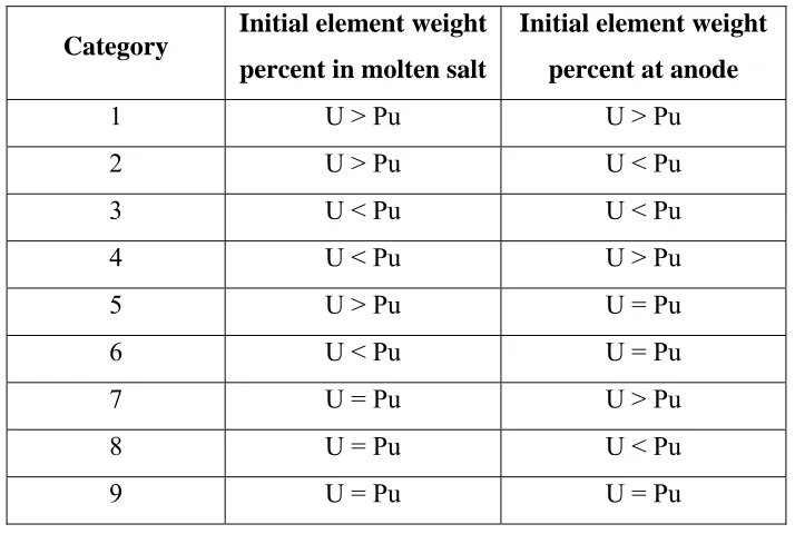
Table 4.6 – Combinations of initial element concentration at anode and molten salt ... 66

Table 4.7 – Input variable space ... 67

Table 4.8 – Latin Hypercube design with optimal spacing for electrorefiner ... 68

Table 4.9 – Electrorefiner mesh characteristics ... 76

Table 4.10 – Molten salt data [25] ... 78

Table 4.11 – Uranium data [26] ... 78

Table 5.1 – Initial electrorefiner inventory for uranium extraction stage – category 1 ... 82

Table 5.2 – Final electrorefiner data for uranium extraction stage – category 1 ... 85

(11)

Table 5.6 – Final electrorefiner data for uranium extraction stage – category 3 ... 94

Table 5.8 – Initial electrorefiner data for uranium and plutonium extraction stage ... 99

Table 5.9 – Results summary for design of experiment ... 107

Table 5.10 – Diffusion layer thickens for left cathode – molten salt interface ... 119

Table 5.11 – Diffusion layer thickens for right cathode – molten salt interface ... 120

Table 5. 12 – Final rotational model for stirrer and cathodes ... 122

Table 5.13 – Final diffusion layer thickness for electrorefiner ... 122

Table 5.14 – Material balance per cathode and operation time for optimum case ... 129

Table 5.15 – Continuous electrorefiner performance ... 132

Table A.1 – Design of experiment results-uranium extraction stage ... 145

Table A.2 – Design of experiment results-uranium and plutonium extraction stage ... 150

(12)

LIST OF FIGURES

Figure 2.1 – Electrochemical processing flowchart [12] ... 16

Figure 2.2 – Electrorefining process [12] ... 19

Figure 2.3 – Standard free energies of formation of fission product, actinide element and electrolyte chlorides at 500 °C ... 21

Figure 2.4 – Concentration profile and diffusion layer thickness ... 31

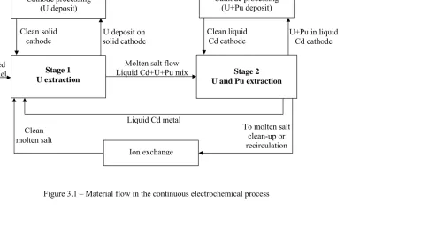
Figure 3.1 – Material flow in the continuous electrochemical process ... 49

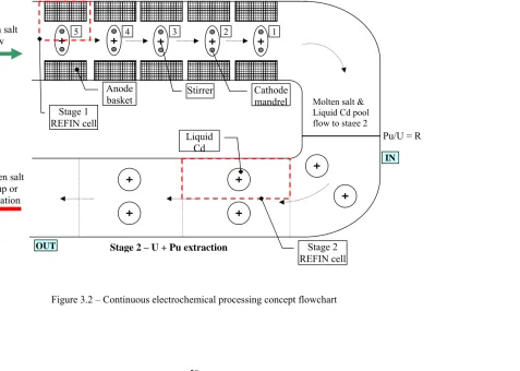
Figure 3.2 – Continuous electrochemical processing concept flowchart ... 50

Figure 3.3 – Cathode assembly used for uranium extraction (top view) ... 51

Figure 3.4 – Cathode mandrel with insulator disc (front view) ... 52

Figure 4.1 – Schematic of electrochemical circuits in continuous operation (front view) ... 58

Figure 4.2 – Electrochemical cell modeled with REFIN code (top view) ... 59

Figure 4.3 – Latin Hypercube design with optimal spacing ... 70

Figure 4.4 – REFIN and ANSYS CFX coupling ... 71

Figure 4.5 – Different electrochemical cell designs ... 74

Figure 4.6 – Final electrochemical cell geometry ... 75

Figure 4.7 – Electrochemical cell mesh ... 77

Figure 5.1 – Element mass in electrorefiner for uranium extraction stage – category 1 ... 83

Figure 5.2 – Element cathode potential for uranium extraction stage – category 1 ... 84

(13)

Figure 5.9 – Element mass in electrorefiner for uranium and plutonium extraction stage – category 4 ... 100

Figure 5.10 – Element cathode potential for uranium and plutonium extraction stage – category 4 ... 101

Figure 5.11 – First stage recovery efficiency and operation time as function of electric current and element concentration ... 103

Figure 5.12 – Overall recovery efficiency and operation time as function of electric current and element concentration ... 104

Figure 5.13 – First stage recovery efficiency vs. operation time ... 105

Figure 5.14 – Global recovery efficiency vs. total operation time ... 106

Figure 5.15 – U volume fraction in molten salt for first stirrer design ... 108

Figure 5.16 – U volume fraction in molten salt for second stirrer design ... 110

Figure 5.17 – U volume fraction in molten salt for final stirrer design at 30 rpm ... 111

Figure 5.18 – U velocity on cathodes and stirrer for final stirrer design at 120 rpm ... 112

(14)

Figure 5.21 – Diffusion layer at right cathode for 60 rpm stirrer rotational velocity ... 117 Figure 5.22 – U velocity for final stirrer design at 60 rpm stirrer rotational velocity ... 118 Figure 5.23 – U concentration profile at left and right cathode surfaces ... 121 Figure 5.24 – Change in element mass per cell per stage for uranium extraction stage – optimum case ... 124 Figure 5.25 – Element cathode potential variation per cell per stage for uranium extraction stage – optimum case ... 125 Figure 5.26 – Change in element mass per cell per stage for uranium and plutonium

extraction stage – optimum case ... 126 Figure 5.27 – Element cathode potential variation per cell per stage for uranium and

(15)

LIST OF SYMBOLS

ai activity of species i

A interfacial area density, (m-1)

Ci concentration of species i, (mol/cm3)

1

C_ε k-ε turbulence model constant, (1.44)

2

C_ε k-ε turbulence model constant, (1.92)

μ

C k-ε turbulence model constant, (0.09) d distance or length, (m)

Di diffusion coefficient of species i, (cm2/s)

E standard electrochemical potential defined by Gibbs free energy, (V) E° standard electrode potential, (V)

F Faraday’s constant, (96,487 Coulomb/mol)

ΔG “standard” Gibbs energy change for a reaction, (kcal/mol) D

f G

Δ free formation energy of selected compound, (kcal/mol)

htot specific total enthalpy, (J/kg) I electric current intensity, (A)

Ji net flux density for species i, (mol/cm2·s)

(16)

Ji,migration flux density due to migration of species i, (mol/cm2·s) k turbulent kinetic energy per unit mass, (m2/s2)

Keq equilibrium constant

m mass of material transported, (kg)

M molar mass, (mol/kg)

MD momentum due to interphase drag force ML momentum due to lift force

MLUB momentum due to wall lubrication force MS momentum due to solids pressure force MTD momentum due to turbulence dispersion force MVM momentum due to virtual mass force

n number of electrons transferred through the external circuit N number of components in mixture

p, pstat static (thermodynamic) pressure, (Pa) p` modified pressure, (Pa)

ptot total pressure, (Pa)

Pk shear production of turbulence, (kg/m·s3)

Pr Prandtl number

Q amount of electric charge, (Coulomb)

(17)

R universal gas constant, (8.3143 J/mol·K)

Re Reynolds number

Rv radial vector from the domain axis of rotation to the wall, (m) SE energy source, (kg/m·s3)

SM momentum source, (kg/m2·s2) SMS mass source, (kg/m3·s)

t time, (s)

T static (thermodynamic) temperature, (K) ui mobility of species i, (cm2·mol/J·s) U vector of velocity Ux,y,z, (m/s) v bulk fluid velocity, (cm/s)

vi velocity of ions in electrolyte, (cm/s)

V volume, (m3)

Xi mole fraction of species i zi charge number of species i

α subscript to indicated that the quantity applies to component α

β subscript to indicated that the quantity applies to component β

ε turbulence dissipation rate, (m2/s3)

Φ electric potential, (V)

(18)

Γ diffusivity, (m2/s)

λ thermal conductivity, (W/m·K)

μ molecular (dynamic) viscosity, (Pa·s) µeff effective viscosity, (Pa·s)

μt turbulent viscosity, (Pa·s)

ρ density, (kg/m3)

σk k-ε turbulence model constant, (1.0)

σε k-ε turbulence model constant, (1.3)

τ shear stress, (Pa)

(19)

LIST OF ABREVIATIONS

ANL Argonne National Laboratory

CFD Computational Fluid Dynamics COEX Combined Extraction Process DOE Department of Energy

ERB-II Experimental Breeder Reactor II KAPL Knolls Atomic Power Laboratory IMSE Integrated Mean Squared Error INL Idaho National Laboratory LWR Light Water Reactor

ORNL Oak Ridge National Laboratory

(20)

Chapter 1 Introduction

A unique feature of nuclear energy is the availability in spent nuclear fuel of

recyclable fissile and fertile materials able to provide new fuel to generate power. When we

recycle paper, glass, plastic or metal we separate useful materials from waste, mainly to

reduce the consumption of fresh raw materials and also to diminish the air and water

pollution. Spent nuclear fuel contains considerable amounts of useful materials. To illustrate

this, the composition of used nuclear fuel is presented in the first section of this chapter.

Furthermore, an overview of reprocessing is given to bring this thesis into context. A

comparison of reprocessing methods, underlining the advantages and disadvantages of

current electrochemical processing technology, is provided for a better understanding of the

motivation of using and improving this technology.

1.1 Nuclear Energy and Spent Nuclear Fuel

One of the most critical topics in today’s society is energy. Major concerns include

resource depletion, impact on air and water pollution, security and cost. Energy generation

affects all aspects of life, from every day tasks to industrial productivity and feeding the

(21)

Conventional nuclear power is based on the nuclear fission reaction to generate

energy. When the fissile uranium-235 isotope absorbs a neutron, the intermediate nuclide

uranium-236 becomes immediately unstable and fissions. The products of this reaction

typically include two fission products, 200 MeV of energy and an average of 2.5 neutrons.

More uranium is bombarded by some of these neutrons to produce energy whereas others are

used to create fissionable plutonium-239 from uranium-238.

Table 1.1 illustrates the composition of the LWR spent nuclear fuel.

Table 1.1 – Composition of LWR spent nuclear fuel [1]

Element or group of elements Percent, by weight Actinides

Uranium 95.6 Plutonium 0.9

Minor Actinides 0.1

Fission products

Stable / Short Lived 3.0

Cesium / Strontium 0.3

Iodine / Technetium 0.1

As it can be seen, the bulk of spent nuclear fuel is reusable material. This represents

(22)

By separating uranium and plutonium from waste, the volume of material to be

disposed of as high-level waste is reduced and also allows uranium and plutonium to be used

as reactor fuel. The spent nuclear fuel is highly toxic because it contains very large inventory

of radioactive isotopes with high radiation energy whose half-lives can be extremely long.

Also, due to its high fissile plutonium content, the proliferation issue becomes important

specifically if any further partitioning is involved.

1.2 Overview of Reprocessing

Reprocessing of spent nuclear fuel refers to the separation process of useful material

from waste. Separation is usually achieved by utilizing the differences in chemical and

physical properties of the substances through the mean of a separating agent. The main goals

for conducting spent fuel separation are to recover useful materials, uranium, plutonium, and

thorium, if present, and to reuse them as fuel, to remove radioactive fission products from

them and to obtain a suitable form for safe and long-term storage. Reprocessing technologies

can be grouped into two main categories: technologies based on aqueous chemistry and those

(23)

1.2.1 History of Reprocessing

Initially, Oak Ridge National Laboratory (ORNL) developed a bismuth phosphate

method of reprocessing spent fuel which was used at Hanford, Washington site beginning in

1944. The process, operating in batches, required several stages including dissolution of

cladding material. Uranium and most of the fission products were discarded as heavy metal

waste whereas plutonium was further purified. Large amounts of waste and chemicals were

generated and no uranium was separated.

Argonne National Laboratory (ANL) developed a new reprocessing method based on

aluminum nitrate in aqueous phase using hexone as solvent for extraction. The process was

continuous but required large amounts of aluminum nitrate.

This method was replaced by plutonium and uranium extraction process (PUREX)

developed by Knolls Atomic Power Laboratory (KAPL) and tested at ORNL in 1950-52 and

used worldwide today. PUREX is a solvent-extraction technique used to extract uranium and

plutonium, independent of each other, from fission products. The method uses nitric acid and

tri-butyl phosphate dissolved in an organic liquid [2]. Adaptations to PUREX have been

applied to become more suitable for treatment of waste and civilian use. Uranium extraction

process (UREX) can be used to remove uranium, which represents most of the volume and

mass of spent nuclear fuel. The PUREX process has been modified to prevent plutonium

extraction by adding acetohydroxamic acid to the extraction and scrub sections, and thus

(24)

ANL developed another related process for recovering transuranic metals from waste,

called TRUEX. This process added another extraction agent to tri-butyl phosphate to remove

transuranic elements from spent fuel and thus to lower alpha activity of the waste. A melt

refining process has been developed in the 1960s to process EBR-II metal fuel in which the

volatile fission products were removed [3]. This process offered partial separation of

actinides and no separate plutonium was recovered. This represents the initial work carried

out in electrochemical processing, also known as pyroprocessing.

1.2.2 Reprocessing Today

Generally, there are two main categories of reprocessing technologies of spent

nuclear fuel. They are either based on aqueous or non-aqueous processes, as presented in

Table 1.2.

Among all these processes, PUREX is the most completely developed and widely

used at present. It is based on the selective affinity of tri-butyl phosphate for uranium and

plutonium. Combined extraction (COEX) of uranium and plutonium was proposed as a

simplification of the PUREX technology. This process, developed in France, leaves

plutonium with uranium to fabricate mixed oxide fuel. Other variations of PUREX are

developed. These recover initially only uranium and then the residual is treated to recover

(25)

Table 1.2 – Main reprocessing technologies of spent nuclear fuel

Aqueous processes Non-aqueous processes

PUREX Electrochemical Processing (also

known as Pyroprocessing)

COEX Fluoride Volatility

UREX - UREX+ - TRUEX -

Supercritical CO2 -

The main difference between variations of UREX+ consists of how plutonium is

mixed with various actinides. UREX technology only separates pure uranium and technetium

and nothing else. Also, experiments using supercritical CO2 technology are ongoing and it is

considered a promising alternative for liquid-liquid extraction systems [4].

The non-aqueous processes include electrochemical processing and fluoride

volatility. Electrochemical processing technologies employ molten salt and molten metal

electrorefining process. Fluoride volatility, which uses the volatility of the uranium

hexafluoride, neptunium hexafluoride, and plutonium hexafluoride to separate them from

(26)

Electrochemical processing techniques to separate actinide elements from waste have

been under development in U. S., notably at ANL, as well as in Russia (at Research Institute

of Atomic Reactors), Japan (at Central Research Institute of Electric Power Industry), India

(at Indira Gandhi Center for Atomic Research), and Republic of Korea (at the Korea Atomic

Energy Research Institute). Production of a separate plutonium stream is very difficult for

this process, since plutonium is collected together with uranium and other elements.

Studies on the molten salt electrorefining process for metallic fuels and oxide

electrowinning process for oxide fuels have been carried out also in India. There,

electrochemical processing studies on uranium alloys have been performed in a

laboratory-scale argon atmosphere facility for molten salt processes [5].

In Japan, basic electrochemical processing research became very important,

especially studies which involved electrochemical and thermodynamic approach.

Electrochemical and related experiments for uranium, plutonium, and other minor actinides

were performed in a large-sized inert glove box built for molten salt processes. Also, a

special attention was given to electrochemical processing of nitride fuels in Japan, due to

their good reactor performance for the future fast breeder reactor [6].

Investigation of continuous operation of electrochemical process has started to

become more important during the last few years. One of the recent U.S. patents presents a

continuous electrorefining process [7]. This approach is focused on uranium separation from

(27)

1.3 Reprocessing Technology Comparison

Several attributes applicable to reprocessing technologies can be compared. A brief

comparison of the most important features of spent fuel reprocessing methods is provided in

the following paragraphs.

Proliferation risk plays a major role in selecting the reprocessing technology. The risk

is mainly given by the possibility of separating pure plutonium from spent nuclear fuel. From

this point of view, electrochemical processing has an advantage over PUREX technology

because it recovers plutonium together with uranium and other transuranic elements

(neptunium, americium, and curium). Also, UREX does not separate plutonium.

Waste toxicity is also important in evaluating a spent fuel reprocessing method. A

concern about PUREX is that neptunium, americium, and curium are kept in waste. These

elements are very toxic and affect the design of geologic repositories. UREX can be an

alternative to PUREX since plutonium is not separated and other elements are kept with

plutonium. Electrochemical processing recovers all the actinides and therefore the remaining

waste is not as long lived as it would otherwise be. Most of these actinides can be consumed

by reactors as fuel and thus the long term threat from waste is reduced.

Another advantage of electrochemical processing over aqueous methods is that the

desired outcome is achieved in fewer steps and the technology is considerably more compact,

allowing on-site reprocessing of reactor waste. This minimizes the burden during spent fuel

(28)

Also, electrochemical processing can be applied to high burn-up fuel and fuel with

little cooling time, as the operation temperature is high. Electrochemical processing does not

use water, which is easily contaminated and also tends to serve as a moderator, but uses

molten salt and molten metals which are known for their fast kinetics and radiation

resistance.

Advanced aqueous methods are best suited to treat spent fuel that is stored and

generated today. The PUREX process only dissolves some types of fuel (oxide fuel) but it

does not dissolve metal fuels. At the same time, electrochemical processing can be adapted to

treat both metal and oxide fuels.

Unlike the PUREX and UREX+ processes, current electrochemical processing

technology relies on batch operation and, therefore, the total throughput of the system is

limited and the uncertainties in total amount of material processed are significant. This is due

to fact that some material remains in the molten salt for several batches until the salt is

processed. The estimated uncertainties, per element, for electrochemical processing are

(29)

Table 1.3 – Estimated uncertainties in electrochemical processing material balance [8]

Element Error [%]

Np 27 %

Pu 6 %

Am 39 %

Cm 12 %

U 13 %

1.4 Electrochemical Processing Modeling Overview

Several models have been developed in order to predict and to keep track of the

material balance in electrochemical processing. Simulation represents a useful tool to

investigate the performance of the electrochemical process. Also, the capability to calculate

the process outcome using modeling saves time and energy.

Models use thermodynamic equilibrium based on the high temperature process

operation and fast kinetics. In 1989 Ackerman developed at ANL, based on the theoretical

model of Johnson, the code called PYRO to calculate mass flow and compositions in

electrochemical processing. The code, written in PASCAL, was based on thermodynamic

equilibrium considerations. Furthermore, the code was extended to include mass tracking of

isotopes and their radioactive decay [9].

Nawada and Bhat developed in 1995 a thermochemical model for application to a

(30)

Next, in 1996, Ahluwalia and Geyer developed at ANL a computer code, named GC,

for flow sheet simulation of electrochemical processing of spent nuclear fuel [9]. The code

utilizes an algorithm for analyzing simultaneous chemical reactions between species

distributed across many phases. They applied the computer code GC to electrochemical

processing flow sheet of LWR oxide fuel.

Researchers at CRIEPI, Japan have developed TRAIL code based on a diffusion

model [9]. This code uses diffusion layer theory in the vicinity of the electrodes.

Diffusion layer thickness was determined based on polarization data measured with

uranium. They assumed fast kinetics at interface between electrode and electrolyte based on

the high temperature of the process. The code assumes a linear concentration profile within

the diffusion layer and uniform concentrations in electrolyte and cadmium.

Models presented above are based on thermodynamic equilibrium or simple diffusion

kinetics. These models work well at low current densities but their accuracy degrades at high

current densities, when kinetic factors become important.

A FORTRAN-based electrorefining model, called REFIN, has been developed based

on a new mathematical model formulated to treat the time-dependent behavior of

multi-component electrochemical systems [9]. The model is able to predict the current density for

each species participating in the electrochemical reactions. The code solves the

electrochemical reactions within the diffusion layer. REFIN has a unique advantage over

(31)

REFIN code can simulate different types of electrodes, such as liquid anode and

liquid / solid cathode. The type of electrode employed in the simulation is defined in the

input file, by specifying the diffusion layer thickness. Seven elements of interest are defined

in this code. These are: uranium, plutonium, neodymium, cadmium, lithium, potassium, and

chlorine.

REFIN code has been benchmarked against Tomczuk et al. experiment performed at

ANL [11]. Tomczuk et al. performed several experiments to investigate the electrodeposition

of uranium and plutonium to solid cathode as part of the electrochemical processing

development. The electrorefiner used in the experiment consisted of a liquid cadmium anode,

a molten LiCl-KCl electrolyte, and a rotating solid cathode. During the experiment five tests

have been performed. In each test the electrorefiner was operated for a preset time at a

selected constant current. The molten salt, liquid anode and solid cathode were analyzed

before and after each test for uranium, plutonium, americium, and rare earths (Ce, Nd, and

Y). The solid cathode was removed after each test. Also, during these tests, the ratio of

plutonium inventory to uranium inventory in the electrorefiner and the PuCl3/ UCl3 ratio in

the electrolyte have been increased by removing pure uranium on the solid cathode.

In the study presented herein, REFIN code was employed to solve mass transfer in

(32)

1.5 Scope of Thesis

The main objective of this thesis was to investigate the feasibility of continuous

electrochemical processing operation for spent nuclear fuel to achieve the desired separation

performance by using computer based simulations. This study focused on computational

simulation of the processes that take place in the electrorefiner, the key equipment of the

electrochemical process.

Since the current electrochemical processing technology relies on batch operation, the

total throughput of the system is inherently limited. Furthermore, nuclear materials

accounting is also difficult because some of the material is held in the molten salt for several

batches until the salt is recovered.

Simulation of the electrochemical reactions at the electrode surfaces was based on the

kinetic modeling capability of a time-dependent one dimensional code, REFIN [9]. The code

was benchmarked against experimental data [11]. REFIN code was used to determine the

mass of uranium deposited at solid cathode and also the amount of uranium and plutonium

collected at liquid cadmium cathode. In addition, the operation time for the electrochemical

process was estimated using REFIN code, based on the operational and geometrical

parameters of the electrorefiner. The flow velocity profiles and chemical concentration

distribution of elements in the molten salt were determined through 3D CFD simulation

using ANSYS CFX-11.0. By solving the mass and momentum transfer in the bulk solution

(33)

Moreover, a design of experiment for computers was performed to investigate the

separation efficiency of the electrochemical process for the proposed concept, using JMP-7.0

statistical software.

Electrochemical processing of spent nuclear fuel plays an important role in the

development of the next generation nuclear reactors and also the technologies that will close

the nuclear fuel cycle. Successful demonstration of the continuous electrochemical

processing leads to development of a new process of reprocessing for spent nuclear fuel that

does not allow pure plutonium separation, which is an important advantage over

conventional aqueous processing. Additionally, this approach offers several improvements

over current batch electrochemical processing operation including larger throughput and

significant safeguards benefit with the reduction of the measurement uncertainties.

Chapter 1 of this thesis presents the motivation for reprocessing spent nuclear fuel

and a brief reprocessing history and technology comparison. The uncertainties in material

balance for electrochemical processing are given to underline the need for a continuous

process development. In Chapter 2, the chemical and physical principles of electrochemical

process and the theory behind the CFD simulation are reviewed. Chapter 3 describes the

continuous electrochemical processing concept proposed in this study. In Chapter 4, the

computational simulation for the continuous concept is presented. The results are shown and

discussed in Chapter 5. The conclusions derived from findings and recommendations for

(34)

Chapter 2 Theory

In order to embark on our explorations of the continuous electrochemical processing

operation concept, we need to understand first the principles that are behind the

electrochemical separation. This chapter begins by presenting the technology and equipment

involved in electrochemical processing of spent nuclear fuel. Next, it provides a description

of the physics and chemistry of the electrochemical processing. Furthermore, a discussion on

design of experiment for computers is given. This technique is used in this study to optimize

the separation efficiency and operation time of the continuous electrochemical processing

concept. Finally, a review of the mathematics of CFD is presented. CFD simulations are

employed to determine the hydrodynamic conditions of the electrochemical process and to

calculate the diffusion layer thickness.

2.1 Electrochemical Processing

2.1.1 Process Overview

Electrochemical processing of spent nuclear fuel refers to the set of operations

(35)

Electrorefining is the most important among them because it separates actinide elements

from the fission products present in the spent nuclear fuel. Other processes are mainly

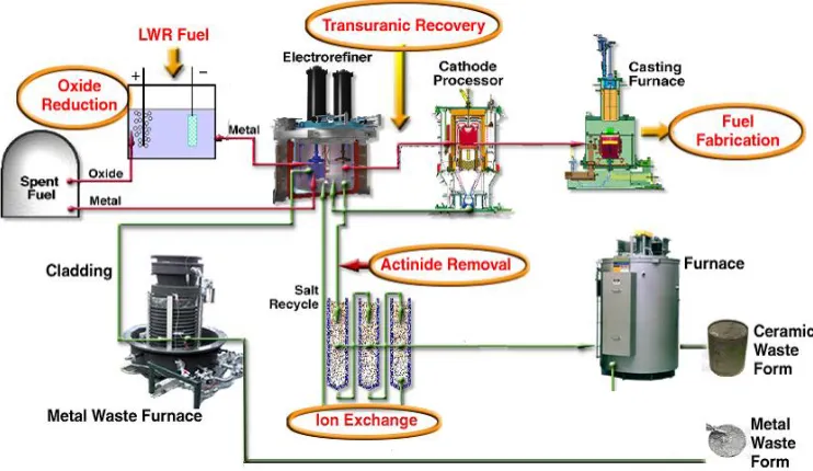
employed to manage the waste. The electrochemical processing flowchart is presented in

Figure 2.1.

Figure 2.1 – Electrochemical processing flowchart [12]

One of the advantages of the electrochemical processing is the use of molten salts as

electrolyte. Besides their fast kinetics, molten salts have a high radiation resistance. Liquid

metals, which can be used as anodes or cathodes, have similar advantages. In the

(36)

brought into contact. The processing operations begin with decladding and chopping the

spent fuel. The chopping operation is performed by a chopper, where the fuel rods are cut

into short lengths. The chopped fuel rod segments are placed in a perforated steel basket,

which represents the anode during the electrorefining operation. For spent fuel from

commercial reactors, which consists of uranium oxide, another step is performed prior to the

electrorefiner, in order to convert the oxide fuel into metallic form. The oxide fuel loaded

into the cathode basket is reduced to produce oxygen gas or CO2 at the anode. This operation

is known as electrolytic oxide reduction.

The electrorefining of spent nuclear fuel is virtually the same as the electrorefining

process used in the minerals industry. During this process an impure metal, which represents

the anode, is electrotransported through an electrolyte to the cathode where it is deposited in

a condition of greater purity. Electrorefining in chloride salt is mainly used to extract

uranium and plutonium. A molten salt medium of LiCl-KCl eutectic is employed and

dissolved actinide chlorides, such as UCl3 and PuCl3, are added to the process. The

electrorefiner operating temperature is typically 500 °C.

After the anode basket is loaded with chopped spent fuel, it is lowered into the molten

salt and virtually pure uranium is collected at a solid mandrel cathode by means of an applied

electric current. It has been observed experimentally that the morphology of the

uranium-plutonium mixture deposited on solid cathode has changed from dendritic form that

(37)

The amorphous deposit is non-adherent on solid cathode [13]. As a result, liquid

cadmium cathode was employed for collecting uranium-plutonium mixture. Other elements,

such as americium, neptunium, curium and some rare-earth fission products are also

collected at the liquid cadmium cathode. In electrochemical process, actinides are recovered

as a group and no pure plutonium is collected at cathode. The fact that the plutonium product

contains some highly radioactive material and it is diluted with uranium discourages weapons

proliferation and undesirable diversion. This represents a major advantage of this technology.

The remaining fission products accumulate in the salt and in the cadmium pool

situated at the bottom of the electrorefiner vessel. The role of the liquid cadmium pool is to

collect the uranium dendrites that drop from the solid cathode during electrorefining. Also, it

acts as an anode during the deposition mode and as an intermediate electrode during the

direct transport mode [14].

The electrorefiner can be operated in three different modes, which can be visualized

in Figure 2.2:

• Anodic Dissolution – in this mode the perforated steel basket, called fuel dissolution

basket, serves as anode and the liquid cadmium pool from the bottom of the

electrorefiner vessel represents the liquid cathode.

• Direct Transport – is the process that takes place when uranium is electrotransported

from solid anode to solid cathode through the molten salt. It has been experimentally

(38)

electrode during the direct transport operation and only a portion of the applied

current passes directly from the anode basket to cathode, through the electrolyte [14].

• Deposition – this is the process of deposition to solid cathode of uranium that has

been dissolved in liquid cadmium pool and molten salt during anodic dissolution

process.

Figure 2.2 – Electrorefining process [12]

The cathode deposit, removed from the electrorefiner, is sent to the cathode

(39)

could be salt, in case of a solid uranium deposit, or liquid cadmium, in case of a liquid

cadmium cathode deposit. The cathode processor product is sufficiently free of impurities to

be used as feed material for the next operational steps, casting furnace and fuel fabrication.

The electrochemical processing of spent nuclear fuel results in two high-level waste

forms, the ceramic waste form and the metal waste form. The ceramic waste form has been

developed to stabilize the active fission products and transuranic elements of the electrolyte.

The ceramic waste form is produced by mixing and blending the waste salt with zeolite. The

salt-loaded zeolite is mixed with borosilicate glass and consolidated at high temperature and

pressure to make the final ceramic waste form. The metal waste form is used to stabilize

noble metal fission products, non-active fuel matrix and cladding materials. The material is

placed in the metal waste furnace and the resulting ingot represents the metal waste form.

2.1.2 Principle of Electrorefining

Electrorefining is the most important step in the electrochemical processing

operation. This is the process where the actinides are separated and recovered from the

fission products in the spent fuel. Electrochemical processing of spent fuel is based on the

partition of the spent fuel elements according to the free energies of formation of selected

chlorides at 500 °C. The chloride electrolyte system is used because it presents the advantage

(40)

Figure 2.3 – Standard free energies of formation of fission product, actinide element and

Δ

G°, (kcal/mole of chlorine at 500°C)

Am, Cm -10 -20 -30 -40 -50 -60 -70 -80 -90 Tc Mo Fe Cd Zr U Np Pu Y Nd Ce La Na Li Sr K Cs

(41)

Three main thermodynamic classes are observed in Figure 2.3, based on the standard

free energies of formation of fission product, actinide element, and electrolyte chlorides at

500 °C. Elements located at the top of Figure 2.3 have relatively unstable chlorides. These

elements include cadmium, cladding hull constituents and the transition-metal fission

products. As a consequence, during electrorefiner operation, these elements remain in the

anode basket and at the end will be part of the metal waste form.

The elements positioned at the bottom of Figure 2.3 have highly stable chlorides.

These elements are completely oxidized to chlorides and accumulate in the molten salt

during the electrorefiner operation. They are periodically removed from the molten salt into

the ceramic waste form by means of ion exchange.

The middle group consists of elements that are electrotransportable to solid or liquid

cathode by means of an externally applied electric current. These elements are those of

interest in the electrochemical processing of spent fuel. Table 2.1 presents an ordered list of

the stabilities of the element chlorides involved in electrochemical processing at 500 °C.

At anode, electric current is used to oxidize metal into the salt phase and to

simultaneously reduce the same amount of chloride from the salt phase to the cathode phase.

By controlling electrotransport phenomenon, a pure uranium deposit can be collected at solid

cathode and a mixed uranium-plutonium-rare-earth metal product can be obtained at liquid

cadmium cathode. During the operation of the electrorefiner, the elements of this group are in

(42)

pairs between salt and metal phases can be determined based on the equilibrium constants for

the reactions between each pair of elements in this group.

Table 2.1 – Free energies of formation of selected chlorides at 500 °C [3, 15]

Element Chloride Free Energy [kcal/mole of chlorine]

CsCl -87.8 KCl -86.7 SrCl2 -84.7

LiCl -82.5 NaCl -81.2 LaCl3 -70.2 PrCl3 -69.0 CeCl3 -68.6 NdCl3 -67.9 YCl3 -65.1 PuCl3 -62.4 NpCl3 -58.1 UCl3 -55.2 ZrCl4 -46.6

CdCl2 -32.3

FeCl2 -29.2

NbCl5 -26.7

(43)

The exchange reaction between any two different metallic elements, M and N, in this

class is given by:

y x NCl 3 y M 3 x N 3 y MCl 3

x ₊ _↔ ₊

(2.1)

For the exchange reaction, the free energy change is given by the following formula:

) MCl ( G 3 x ) NCl ( G 3 y

G= Δ _f° _y − Δ _f° _x

Δ (2.2)

where )ΔG_f°(⋅ _{represents the free energy of formation of that compound.}

The equilibrium constant for the exchange reaction is determined using the free energy

change: ) RT / G exp(

K_eq = −Δ (2.3)

Also, the equilibrium constant can be written using the activity coefficients of the reactants

and products of the exchange reaction, as follows:

3 / y N 3 / x MCl 3 / x M 3 / y NCl eq ) a ( ) a ( ) a ( ) a ( K x y = (2.4)

where ai represents the activity of species i.

Expressing the activity of species i as the product between the activity coefficient γi and the

mole fraction Xi, Equation (2.4) becomes:

3 / x MCl M 3 / y N NCl 3 / x MCl M 3 / y N NCl eq x y x y X X X X

K _⎟⎟

⎠ ⎞ ⎜ ⎜ ⎝ ⎛ ⎟⎟ ⎠ ⎞ ⎜⎜ ⎝ ⎛ ⎟ ⎟ ⎠ ⎞ ⎜ ⎜ ⎝ ⎛ γ γ ⎟⎟ ⎠ ⎞ ⎜⎜ ⎝ ⎛ γ γ

(44)

The equilibrium condition given by Equation (2.5) is satisfied at each interface by the

element distribution in the salt and metal phases. The amount of electric charge passed gives

the amount of material in the anode and cathode metal phases.

The Nernst equation, which relates the potential generated by an electrochemical cell to the

standard potential E0 and the activities of the species involved in the cell reaction, is then

given by: 3 / y N 3 / x MCl 3 / x M 3 / y NCl ) a ( ) a ( ) a ( ) a ( ln nF RT E E x y −

= ° _(2.6)

where R is the universal gas constant, F is the Faraday’s constant, T is the absolute

temperature and n represents the number of electrons transferred through the external circuit

for the reaction.

Table 2.2 shows the activity coefficients of actinides and rare earths at infinite dilution in

(45)

Table 2.2 – Activity coefficient of actinides and rare earths at infinite dilution [9]

Element Coefficient in

liquid Cd Chloride

Coefficient in LiCl-KCl

U 75 UCl3 ₅_.₇₉_⋅₁₀−3

Np ₈_.₂_⋅₁₀−3 _{NpCl3 -}

Pu ₁_.₃₈_⋅₁₀−4 _PuCl3 ₆_.₆₂_⋅₁₀−3

Am _≈₂_⋅₁₀−6 _{- -}

Cm _≈₃_⋅₁₀−5 _{- -}

Ce ₉_.₇₆_⋅₁₀−9 _CeCl3 ₁_.₅_⋅₁₀−3

La ₃_.₅₈_⋅₁₀−9 _LaCl3 ₄_.₇_⋅₁₀−3

Pr ₁_.₈_⋅₁₀−8 _PrCl3 ₃_.₃_⋅₁₀−3

Nd _≈₆_⋅₁₀−9 _NdCl3 ₁_.₈_⋅₁₀−2

Y - YCl3 ₆_.₃_⋅₁₀−6

2.1.3 Electrode Reactions

The electrode at which positive charge enters the solution and the reactant is said to

be oxidized is termed the anode. Similarly, the cathode represents the electrode where the

negative charge enters the electrolyte solution or the positive charge leaves the solution. In

this case, the reactant is reduced. General anode and cathode reactions are:

−

+

→M (moltensalt) z e

) metal (

M0 zi _i (Anode process) (2.7)

) metal ( M e z ) salt molten ( M 0 i

zi + −→ (Cathode process) (2.8)

(46)

The reaction at the anode involves removal of zi electrons per atom and, therefore, the

i

z

M ions are formed in the salt phase. The removed electrons are conducted through an

external circuit to the cathode, where the metal is formed. The amount of material being

electrotransported from the anode to the cathode is proportional to the electric charge passed

in the electric circuit. The electric charge is given by the product of the electric current and

time, thus the mass of material transported is given by:

F n Q M m ⋅ ⋅ = (2.9)

where M is the molar mass of the element, Q represents the amount of charge passed and n is

the number of electrons involved in the reaction.

Equation (2.9) is known as the Faraday’s first law and is used to determine the amount of

material deposited at the cathode. Expressing the electric charge as the product of the electric

current and time, the mass of material electrodeposited at the electrode is given by:

t I const F n t I M

m = ⋅ ⋅

⋅ ⋅ ⋅

= (2.10)

where I is the value of the applied electric current and t represents the operation time.

Equation (2.10) shows that the amount of material collected at the cathode is directly

proportional to the molar mass of the element, the applied electric current, and time of

(47)

2.1.4 Mass Transport Mechanisms

Similarly to the movement of electrons in a conductor in response to an electric field,

ions move in an electrolyte in response to an electric field, and also concentration gradients

and bulk fluid motion. The movement of ions due to the electric field is called migration. In

this case, the electric field represents the driving force for the motion of the charged particles.

The process of progression of ions from an area with high concentration to an area of lower

concentration represents diffusion. The bulk movement of a fluid is convection. The sum of

all these processes gives the net flux of ions.

The velocity of ions in the electrolyte as a consequence of the electric field represents

the migration velocity, which can be expressed as:

Φ ∇ − = zuF

v_i _i _i (2.11)

where ui represents the mobility of species i and Ф is the potential in solution. Mobility is the

proportionality factor that indicates how fast the ions move as a result of the electric current.

Using Equation (2.11), the flux density due to migration is given by:

Φ ∇ −

=

= _i _i _i _i _i

migration ,

i v C z u FC

J (2.12)

where Ci represents the concentration of the species i.

The application of an electric current creates the movement of all ions in molten salt

by migration. As a result, a change in concentration is observed across the molten salt. These

concentration gradients drive mass transport by process of diffusion, in addition to

(48)

The flux density due to diffusion is:

i i diffusion ,

i D C

J =− ∇ (2.13)

where Di is the diffusion coefficient of species i.

Convection refers to the movement of ions in the bulk solution. It can be caused by

density gradients (natural convection) or by mechanical stirring (forced convection). Also,

convection can be turbulent, when the motion is chaotic, or laminar, described by smooth,

constant fluid motion. The Reynolds number characterizes whether the flow conditions lead

to laminar (low Reynolds numbers) or turbulent flow (high Reynolds numbers).

The flux density by convection of a species i is expressed as:

v C

J_i_,_convection = _i (2.14)

where v represents the bulk fluid velocity.

Combining the Equations (2.12), (2.13), and (2.14) the net flux density is obtained:

v C C D FC u z

J_i =− _i _i _i∇Φ− _i∇ _i + _i (2.15)

Equation (2.15) shows that mass transport mechanisms in an electrochemical cell are

migration, diffusion and convection [16].

The mobility of chemical species can be expressed using the Nernst – Einstein relation, as:

i i RTu

D = (2.16)

Inserting Equation (2.16) in Equation (2.15), the net flux density is given by:

v C C D C D z RT F

(49)

From Equation (2.17), the current in solution can be obtained from the flux density of

charged species:

∑

=

i i iFJ

z

I (2.18)

where Ji represents the flux density of species i.

2.1.5 Diffusion Layer

Although there is fluid motion in the bulk solution, there is a thin layer adjacent to the

electrode where the molten salt is stationary. In the bulk solution, the governing mass

transport mechanisms are convection and migration. Diffusion is almost negligible in the

bulk solution because the concentration is approximately constant. The ions travel by

convection and migration from the bulk up to the stationary layer and then cross the layer by

diffusion. This thin layer adjacent to the electrode surface is called diffusion layer.

The diffusion layer represents the region in the vicinity of an electrode where the

concentrations are different from the values in the bulk solution [17]. The exact value of the

diffusion layer thickness is hard to obtain since it represents an approximate property. The

diffusion layer thickness depends strongly on the effectiveness of the forced convection,

being smaller when the convection is more intense [18]. The method of determining the

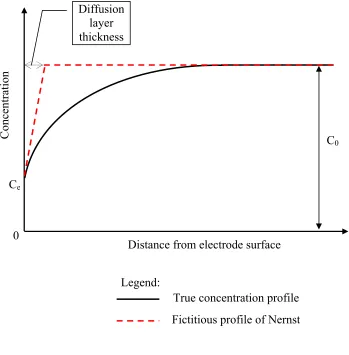
diffusion layer thickness is presented below. Figure 2.4 shows the concentration profile near

the electrode surface. The concentration profile would be constant, equal to C0, if no electric

(50)

When the electric current is applied the electrode surface concentration decreases to

Ce. The thickness of diffusion layer is given by the distance from the electrode surface to the

intersection of the tangent to the true concentration profile at interface and the straight line

extension of the concentration in the bulk solution [17, 19].

Figure 2.4 – Concentration profile and diffusion layer thickness Distance from electrode surface

C0

Ce

Diffusion layer thickness

Concentration

Legend:

(51)

2.2 Design of Experiment for Computers

Nowadays, experiments are used widely to study and optimize processes and systems.

Usually, the goals of experiments performed in modern industry and engineering are to

improve the quality of products, to reduce the operation time and overall costs of the process.

Experiments are categorized as physical or computer experiments. Typically, an experiment

is performed in a laboratory. This type of experiment is called a physical experiment. During

the past years, conducting an experiment with appropriate computer hardware and software

became increasingly popular. In most of the cases a computer experiment is feasible when

physical experiments are impossible to implement. Such examples may include experiments

that are time consuming, have a number of factors that is too large to perform a physical

experiment or are too expensive to run on the scale needed for answering a particular

research question. Whereas physical experiments measure a stochastic response, computer

experiments yield a deterministic answer for a given set of input conditions. Therefore, most

of the traditional tools of design of experiment (blocking, replication and randomization) are

not used in solving computer experiments [20].

2.2.1 Factors and Experimental Domain

A factor represents a variable that can be controllable and is of interest in the

experiment. Usually, a factor is called an input variable in a computer experiment [21].

(52)

Factors can be quantitative or qualitative. A quantitative factor is one that has a

numerical value and can vary in a range or interval whereas qualitative or categorical factors

are those defined as categories of different materials, operators, etc. Most of the factors

employed in a computer experiment are quantitative.

The space where the factors take values is defined as the experimental domain [21].

There may be several specific values within the experimental domain where the factor is

tested. An experimental domain can be defined by two (low and high) or more specific

values. These particular values represent the levels of that factor. In computer experiment,

the experimental domain is also defined as the input variable space. A run is described by the

implementation of one of the possible combinations of levels of the factors. The result of a

run represents the response or the output, for computer experiments. Like factors, the

response of an experiment can be quantitative or qualitative, based on the objective of the

experiment.

2.2.2 Experimental Designs for Computers

Selection of an experimental design is a key issue in performing a computer

experiment. Classical designs are abandoned when performing computer experiments in

favor of others that treat all the regions of the design space equally. The type of design that

fills the space of experiment by spreading the points evenly throughout the experimental

(53)

There are several space-filling designs that can be employed when performing a computer

experiment [22], such as:

• Sphere Packing Design;

• Uniform Design;

• Latin Hypercube Design;

• Minimum Potential Design;

• Maximum Entropy Design;

• Gaussian Process IMSE Optimal Design.

Sphere Packing design tries to spread the points as much as possible in the input variable

space by maximizing the minimum distance between pairs of design points. This operation is

done without any constrains. Uniform design minimizes the discrepancy between the design

points. This does not always result in an even spacing of the factor levels. Latin Hypercube

design assigns for each factor a number of levels equal to the number of runs performed in

the experimental design. The levels are spaced evenly throughout the variable domain.

Compared to the sphere packing design, Latin Hypercube design maximizes the minimum

distance between points maintaining the even spacing between factor levels. Minimum

Potential design spreads points out inside a sphere. This type of design has spherical

symmetry and uniform spacing. Maximum Entropy design optimizes a measure of the

amount of information contained in an experiment. Gaussian Process IMSE Optimal design

(54)

2.3 Three dimensional CFD Modeling

Computational Fluid Dynamics, a computer based tool, is used to simulate the

behavior of systems involving fluid flow, multiphase and multicomponent interactions, heat

transfer and other physical processes. Current advances in computer power and performance

allow saving time and effort in creating a CFD model. Nowadays, CFD represents a

recognized tool for research and industry. Performing a CFD simulation assumes several

steps. First of all, the geometry is created and the required mesh is generated, depending on

the objective of the simulation. The next step is to specify the physics of the problem that has

to be investigated by creating the input file for solver. After that, the CFD problem is solved

and the results are processed.

The CFD tool used in this study to solve the mass and momentum transfer in bulk solution is

ANSYS CFX-11.0. This represents a finite element analysis tool developed by ANSYS, Inc.

2.3.1 Basic Equations

The set of equation solved by ANSYS CFX are the unsteady Navier-Stokes equations

in their conservation form [23]. The instantaneous equations of mass, momentum and energy

conservation are averaged, for turbulent flows, leading to additional terms.

Before presenting the equations, several mathematical notations are given.

Gradient operator

(55)

k z j y i x ∂ φ ∂ + ∂ φ ∂ + ∂ φ ∂ = φ ∇ (2.19) Divergence operator

For a vector functionU

(

x,y,z

)

, the divergence is given by:

z U y U x U

U x y z

∂ ∂ + ∂ ∂ + ∂ ∂ = •

∇ (2.20)

Dyadic operator

The dyadic operator of two vectors, U and V, is given by:

⎥ ⎥ ⎥ ⎦ ⎤ ⎢ ⎢ ⎢ ⎣ ⎡ = ⊗ z z y z x z z y y y x y z x y x x x V U V U V U V U V U V U V U V U V U V

U (2.21)

The instantaneous equation of mass is:

( )

U 0

t +∇• ρ =

∂ ρ ∂

(2.22)

where ρ is the density and U is the velocity vector.

The momentum equation is given by:

( )

₍

₎

M S p U U t

U ₊_∇_• _ρ _⊗ ₌_−∇ ₊_∇_•_τ₊

∂ ρ ∂

(2.23)

where p is the static pressure, τ is the shear stress and SM is the momentum source.

The term ∇•

(

ρU⊗U

)

in Equation (2.23) can be expressed in the specific tensor notation,

(56)

(

)

(

)

(

)

(

)

(

)

(

)

(

)

(

)

(

)

(

)

⎥ ⎥ ⎥ ⎥ ⎥ ⎥ ⎥ ⎦ ⎤ ⎢ ⎢ ⎢ ⎢ ⎢ ⎢ ⎢ ⎣ ⎡ ρ ∂ ∂ + ρ ∂ ∂ + ρ ∂ ∂ ρ ∂ ∂ + ρ ∂ ∂ + ρ ∂ ∂ ρ ∂ ∂ + ρ ∂ ∂ + ρ ∂ ∂ = ⊗ ρ • ∇ z z z y z x y z y y y x x z x y x x U U z U U y U U x U U z U U y U U x U U z U U y U U x U

U (2.24)

The total energy equation can be written as:

(

)

₍

₎

₍

₎

₍

₎

E M tot

tot _Uh _T _U _U _S _S

t p t

h ₊_∇_• _ρ ₌_∇_• _λ_∇ ₊_∇_• _•_τ ₊ _• ₊

∂ ∂ − ∂ ρ ∂ (2.25)

where htot is the total enthalpy, λ represents thermal conductivity, T is temperature, and SE is

the energy source. The term U•S_Mrepresents the work due to external momentum sources.

This term is currently neglected in ANSYS-CFX. The term ∇•

(

U•τ

)

represents the work

due to viscous stresses.

2.3.2 Boundary Conditions

To be able to solve a CFD problem, we have to specify boundary conditions. The

type of boundary condition employed in the investigation of the diffusion layer thickness is

wall. There are several types of boundary conditions for wall that can be specified in

ANSYS-CFX. Those used herein are No Slip (Not Moving, no Wall Velocity) and No Slip

(57)

Wall - No Slip (Not Moving, no Wall Velocity) Boundary Condition

This type of boundary condition is used for the molten salt domain boundary. In this case, the

velocity of the electrolyte at the wall boundary is set to zero, and, therefore, the boundary

condition for the velocity is:

0

U_Wall = (2.26)

Wall - No Slip (Moving, with Wall Velocity) Boundary Condition

As mentioned in a previous section, the thickness of the diffusion layer strongly depends on

the forced convection. In an electrochemical cell, both the cathodes and the stirrer are used to

mix the molten salt and to create suitable conditions for the electrochemical process.

For this type of boundary condition, the molten salt at the wall boundary moves with the

same velocity as the wall. Three options are available in ANSYS-CFX for the wall velocity:

• Cartesian Components:

In this case, the user can specify Cartesian components in a local or global coordinate frame:

k W j V i U

U_Wall = _spec + _spec + _spec (2.27)

• Cylindrical Components:

Cylindrical components are specified in a local cylindrical coordinate system and these are

transformed by ANSYS-CFX into the global Cartesian coordinate system:

zˆ U ˆ U rˆ U

U_Wall = _r_,_spec + _θ_,_specθ+ _z_,_spec (2.28)

• Rotating Wall:

(58)

v

Wall R

U =−ω (2.29)

where ω is the angular velocity of the domain and Rv is the radial vector from the domain

axis of rotation to the wall.

The rotating wall boundary condition has been used for the cathodes and stirrer in this thesis.

Different values and directions can be specified for each of them. The ANSYS solver

transforms the wall velocity specified by user into Cartesian components.

2.3.3 Turbulence Model

Fluctuations in time and space of the fluid represent turbulence. Turbulence occurs

when the inertia forces in the fluid are more significant compared to the viscous forces.

Turbulence modeling is an important issue in CFD simulations. The turbulence model used

in CFD simulation of electrochemical cell is the k-epsilon model. The k-epsilon model is one

of the most common models in turbulence. It is a two-equation model in which transport

equations are solved for the turbulent kinetic energy k and its dissipation rate ε. The

turbulence kinetic energy k is defined as the variance of fluctuations in velocity.

The continuity equation for k-ε model is given by:

( )

U 0

t +∇• ρ =

∂ ρ ∂

(2.30)

The momentum equation is expressed as:

(

U U

)

(

U

)

p'

(

U

)

B

t

U T

eff

eff∇ =−∇ +∇• μ ∇ +

(59)

where B is the body forces, µeff is the effective viscosity, p′ is the modified pressure, equal

to p in ANSYS, by default.

In the k-ε model, the effective viscosity accounting for turbulence is expressed as:

ε ρ + μ = μ + μ =

μ_eff _t C_μ k2 (2.32)

where Cµ is a constant and µt is the turbulence viscosity.

Writing the differential transport equations for the turbulence kinetic energy:

( )

₍

₎

₊ ₋_ρε ⎥ ⎦ ⎤ ⎢ ⎣ ⎡ ∇ ⎟⎟ ⎠ ⎞ ⎜⎜ ⎝ ⎛ σ μ + μ • ∇ = ρ • ∇ + ∂ ρ ∂ k k

t _k _P

Uk t

k

(2.33)

and for the turbulence dissipation rate:

( )

₍

₎

₊ ε

₍

₋ _ρε

₎

⎥ ⎦ ⎤ ⎢ ⎣ ⎡ ε ∇ ⎟⎟ ⎠ ⎞ ⎜⎜ ⎝ ⎛ σ μ + μ • ∇ = ε ρ • ∇ + ∂ ρε ∂ ε ε ε 2 k 1

t _C _P _C

k U

t (2.34)

the values of k and ε are determined.

In Equations (2.33) and (2.34) C_ε₁,C_ε₂_,σ_k,σ_ε are constants and Pk represents the

(60)

2.3.4 Component Model

In ANSYS CFX two separate flow models are available, an Eulerian-Eulerian

multiphase model and a Lagrangian Particle Tracking multiphase model [23]. For

Eulerian-Eulerian model two distinct sub-models can be used, the homogeneous model and the

inter-fluid transfer (inhomogeneous) model. In this study, the inhomogeneous model has been

employed.

Several notations are given before presenting the model. First, the volume fraction of

component α is denoted rα. The volume occupied by component α in a small volume V

around a point where the volume fraction is rα is given by:

V r

V_α = _α (2.35)

The mixture density ρm is defined as:

∑

α α α

ρ =

ρ_m r (2.36)

The total pressure is given by:

2 stat

tot r U

2 1 p

p _α _α _α

α

ρ +

=

∑

(2.37)

where pstat represents the static (thermodynamic) pressure, rα is the volume fraction for

component α, ρα is the density of component α and Uα is the velocity magnitude for

component α.

In the inhomogeneous model the momentum, heat and mass interfacial transfer

(61)

interfacial area per unit volume, denoted as the interfacial area density Aαβ. Interfacial

transfer can be modeled using particle or mixture models. Mixture model has been used in

this thesis to model the uranium and molten salt solution in the electrorefiner. The surface

area per unit volume is determined as:

αβ β α αβ = d r r

A (2.38)

where dαβ is the interfacial length scale.

Interphase transfer coefficients can be correlated to give the mixture Reynolds

number and Prandtl number, as follows:

αβ αβ α β αβ αβ _μ − ρ

= U U d

Re (2.39)

αβ αβ

αβ _λ

μ

= Cp

Pr (2.40)

where ραβ, µαβ, Cpαβ, and λαβ are the density, viscosity, specific heat capacity and thermal

conductivity of the mixture. These are defined as:

β β α α

αβ = ρ + ρ

ρ r r (2.41)

β β α α

αβ = μ + μ

μ r r (2.42)

The momentum and mass transfer equations for the inhomogeneous model in ANSYS CFX

A Study of Continuous Electrochemical Processing Operation Feasibility for Spent Nuclear Fuel

ABSTRACT

DEDICATION

BIOGRAPHY

ACKNOWLEDGMENTS

TABLE OF CONTENTS

LIST OF TABLES

LIST OF FIGURES

LIST OF SYMBOLS

LIST OF ABREVIATIONS

Chapter 1 Introduction

1.1 Nuclear Energy and Spent Nuclear Fuel

1.2 Overview of Reprocessing

1.2.1 History of Reprocessing

1.2.2 Reprocessing Today

1.3 Reprocessing Technology Comparison

1.4 Electrochemical Processing Modeling Overview

1.5 Scope of Thesis

Chapter 2 Theory

2.1 Electrochemical Processing

2.1.1 Process Overview

2.1.2 Principle of Electrorefining

2.1.3 Electrode Reactions

2.1.4 Mass Transport Mechanisms

∑

2.1.5 Diffusion Layer

2.2 Design of Experiment for Computers

2.2.1 Factors and Experimental Domain

2.2.2 Experimental Designs for Computers

2.3 Three dimensional CFD Modeling

2.3.1 Basic Equations

(

)

( )

( )

(

)

(

)

(

)

(

)

(

)

(

)

(

)

(

)

(

)

(

)

(

)

(

)

(

)

(

)

(

)

(

)

(

)

2.3.2 Boundary Conditions

2.3.3 Turbulence Model

( )

(

)

(

)

(

)

( )

(

₍

₎

₍

₎

₍

₎

₍

₎

₍

₎

₍

₎

₍

₎