Seismic Fragility Analysis for Structures, Systems, and Components of Nuclear Power Plants: Part I — Issues Identified in Engineering Practice

(1)

SEISMIC FRAGILITY ANALYSIS FOR STRUCTURES, SYSTEMS, AND

COMPONENTS OF NUCLEAR POWER PLANTS: PART I — ISSUES

IDENTIFIED IN ENGINEERING PRACTICE

Shunhao Ni1, Zhen Cai 2, Wei-Chau Xie 3, Mahesh D. Pandey3, Wei Liu4, and Ming Han5

1

Civil Engineering Analyst, Candu Energy Inc., Canada

2

Research Assistant, Department of Civil & Environmental Engineering, University of Waterloo, Canada

3

Professor, Department of Civil & Environmental Engineering, University of Waterloo, Canada

4

Candu Energy Inc., Canada (Current: China Nuclear Power Engineering Co., Ltd., China)

5

Director, Civil and Project Engineering, Candu Energy Inc., Canada

ABSTRACT

Seismic Fragility Analysis (FA) has been widely used to calculate the seismic capacities of Structures, Systems, and Components (SSCs) of Nuclear Power Plants (NPPs). The seismic capacity of individual SSC from the FA, in terms of seismic fragility curves or High Confidence of Low Probability of Failure (HCLPF) value, is utilized as an input to Seismic Margin Assessment (SMA) or Seismic Probabilistic Risk Assessment (SPRA) of an NPP. In the seismic FA, a single ground-motion parameter, such as Peak Ground Acceleration (PGA), Spectral Acceleration (SA), or the averaged SA over a frequency range of interest, is used to represent the seismic capacity of an SSC. However, a number of deficiencies of the FA, due to the use of a single ground-motion parameter, have been recognized in the engineering practice of nuclear power industry.

In this study, the deficiencies of the FA methodology, in which a single ground-motion parameter is used to represent the seismic capacity, are identified and discussed from the point of view of engineering practice. A case study has been performed to obtain a general observation that the fragility curves or HCLPF seismic capacities obtained from the FA method are significantly influenced by a number of factors, such as the input spectral shape, ground-motion parameter selected, the characteristics of the supporting structures. A methodology to improve the current FA and to eliminate the deficiencies will be proposed and presented in a separate study: Part II — Use of Multiple Ground-Motion Parameters.

Keywords: Seismic Fragility Analysis, Seismic Margin Assessment, Seismic Probabilistic Risk Assessment

INTRODUCTION

Seismic Fragility Analysis (FA) has been widely used to calculate the seismic capacities of Structures, Systems, and Components (SSCs) of Nuclear Power Plants (NPPs) (EPRI, 1994, EPRI, 2002, EPRI, 2009). The seismic capacity of individual SSC from the FA, in terms of seismic fragility curves or High Confidence of Low Probability of Failure (HCLPF) value, is utilized as an input to Seismic Margin Assessment (SMA) or Seismic Probabilistic Risk Assessment (SPRA) of an NPP. The results of SMA or SPRA are then used by regulators and utilities for their risk-informed decision making.

(2)

23rdConference on Structural Mechanics in Reactor Technology Manchester, United Kingdom - August 10-14, 2015 Division VII

deficiencies have prevented the nuclear industry from accurately predicting the seismic capacity and risk of an NPP.

In this study, the deficiencies of the FA methodology, in which a single ground-motion parameter is used to represent the seismic capacity, are identified and discussed from the point of view of engineering practice. A case study has been performed to obtain a general observation that the fragility curves or HCLPF seismic capacities obtained from the FA method are significantly influenced by a number of factors, such as the input spectral shape, ground-motion parameter selected, the characteristics of the supporting structures. A methodology to improve the current FA and to eliminate the deficiencies will be proposed and presented in a separate study: Part II — Use of Multiple Ground-Motion Parameters.

SEISMIC FRAGILITY ANALYSIS

Seismic fragility of the SSC is defined as the probability that the seismic capacity in terms of a

Ground-Motion Parameter (GMP) Aof a SSC is less than a given threshold aof that GMP, i.e.,

{

A

a

GMP

a

}

P

a

p

_F

(

)

=

<

=

. (1)

The GMP seismic capacity Aof a SSC is often expressed as a product of three variables, i.e.,

U R m

A

=

ε

, (2)

where Amis the median GMP seismic capacity, !Ris a random variable representing inherent randomness

(aleatory uncertainty) of A, and !Uis a random variable representing uncertainty (epistemic uncertainty) of

Adue to lack of knowledge. The random variables !Rand !Uare taken to be lognormally distributed with

unit median values and with logarithmic standard deviations of "Rand "U, respectively.

Based on equation (2) and the assumption that !Rand !Uare lognormally distributed, the seismic fragility

curve, i.e., the probability of failure given a GMP threshold aat a confidence level Q=q, is expressed as

(Kennedy and Ravindra, 1984)

{

}

( )

            ₊ _Φ Φ = = = < = − R U m F q A a q Q a GMP a A P q a p

β

1 ) ln( , ) ,

( . (3)

!"#$%&'()*"#+,-.#/#+0-#1('"21#3*4#1('"2'42#"*45'6#2)1(4)7&()*"#3&"8()*"9#The confidence levels Qare often taken as several discrete values, such as 5%, 50%, and 95%. Equation (3) gives a family of seismic fragility curves for various levels of confidence, as shown in Figure 1.

Take 5% probability of failure and 95% confidence level, and solve for a, in equation (3), a High

Confidence of Low Probability of Failure (HCLPF) seismic capacity in terms of a selected GMPacan be

obtained (EPRI, 1994)

( R U)

e A

(3)

Figure 1. Fragility Curves

As can be seen in equations (3) and (4), to calculate the seismic fragility curves and the HCLPF seismic capacity of a SSC, the major task is to determine the median capacity Am, and the associated randomness "Rand uncertainty "U.

In the determination of Am,"R, and "U, an intermediate random variable, the factor of safety F, is often

used. It describes the level that the GMP seismic capacity A is above the reference earthquake level in terms of the same GMP quantity ARef, and is defined as

. (5)

The physical meaning of Fis the ratio of actual seismic capacity of SSC to actual response (demand) of the SSC due to reference earthquake. The reference earthquake is usually represented by a smoothed response spectrum such as Review Level Earthquake (RLE), which has a specified GMP of ARef. In

engineering practice, the factor of safetyFis a product of a number of sub-factors of safety accounting for strength, inelastic energy absorption, and responses of SSCs. The associated uncertainties of Fcan be obtained by using testing and analytical methods, or a combination of them, such as second moment procedure and Monte Carlo simulation (EPRI, 1994).

DEFICIENCIES IN EXISTING SEISMIC FRAGILITY ANALYSIS

(4)

1. Reference Earthquake. As discussed above, the reference earthquake is usually represented by a

smoothed response spectrum, which has a specified value of the selected GMP, such as PGA or SA. This smoothed response spectrum is used as the seismic input to obtain the seismic demand of the SSC, which is part of the determination of the factor of safety in equation (5). The specified

value of the selected GMP is the reference quantity ARef in equation (5). Assume that there are

two reference earthquakes, i.e., the smoothed response spectra, having different spectral shapes

but the same ARef, e.g., PGA, the resulting factors of safety and the associated uncertainties of the

SSC based on these two reference earthquakes could be very different since the response of the SSC largely depends on the spectral shape of the input response spectrum. This usually results in inconsistent seismic fragility curves and HCLPF seismic capacities of the SSC.

2. Ground-Motion Parameter. In the existing seismic fragility analysis, a single GMP is used to

represent the seismic capacity of a SSC. Ideally, the seismic capacity of a SSC should be an intrinsic property of the SSC and then independent of the seismic input. In engineering practice, a single GMP, which is deemed to be much correlated with the SSC response, is often used to characterize the seismic capacity. However, this characterization can never be complete due to the fact that the SSCs are dynamically complicated.

CASE STUDY

In this section, a case study for a typical heat exchanger is conducted to demonstrate the deficiencies in the existing fragility analysis method. To eliminate these deficiencies from the mechanism, a methodology is proposed and presented in a separate study: Part II — Use of Multiple Ground-Motion Parameters, using the same heat exchanger case.

The heat exchanger data used in this study is based on the fragility analysis example of a horizontal heat exchanger presented in Section 8 of EPRI (1994). Configuration details of the heat exchanger are shown in Figure 2 and the properties are listed in Table 1.

The heat exchanger has a diameter of 8 feet, a length of 30 feet, and is supported by three equally spaced saddles. Each saddle is secured to the concrete floor by three sets of 2 cast-in-place anchor bolts. Two of the saddle base plates (Support S1) have slotted holes, which allow the thermal expansion of the tank in the longitudinal direction. Each saddle has four stiffener plates to increase the rigidity of the heat exchanger in the longitudinal direction. A total weight of 110 kips is estimated for the exchanger. The heat exchanger is assumed to be located at the ground level on a rock site, and will be subjected to tri-directional excitations during seismic events.

Modal analysis has shown that the longitudinal and transverse vibration frequencies of the heat exchanger are 8.15 Hz and 25.4 Hz, respectively. Since the heat exchanger is very rigid in the vertical direction, spectral acceleration in the vertical direction can be approximated by PGA.

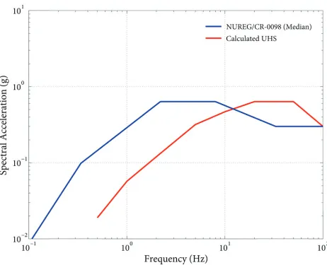
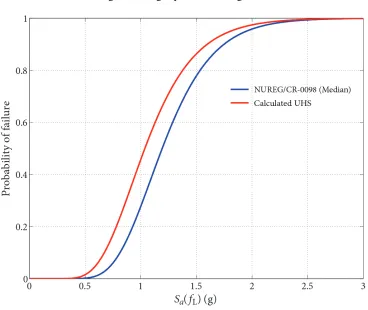
By using different reference earthquakes, i.e., a Uniform Hazard Spectrum (UHS) and a NUREG/CR-0098 median spectrum, as shown in Figure 3, for the fragility analysis, inconsistent fragility curves with a GMP of PGA have been obtained, as shown in Figure 4. As a result, the HCLPF seismic capacities in terms of PGA for the heat exchanger are also different: 0.26g for the NUREG/CR-0098 median spectrum and 0.34g for the UHS (a difference of 24%).

(5)

(6)

(7)

Figure 3. Reference Earthquakes for Fragility Analysis

To reduce this difference, the SA at dominant frequency of the heat exchanger has been used as the GMP. As shown in Figure 5, the difference between the fragility curves using the NUREG/CR-0098 median spectrum and the UHS for the GMP of SA is smaller than that for the PGA. A reduced difference can also be observed from the resulting HCLPF seismic capacity: 0.60g for the NUREG/CR-0098 median spectrum and 0.47g for the UHS (a difference of 22%).

(8)

Figure 4. Fragility Curves Using PGA

(9)

CONCLUSION

In this study, two major deficiencies have been observed in the existing fragility analysis methodology and are discussed with an example of a horizontal heat exchanger. The reference earthquakes and the ground-motion parameters (GMP) selected jointly induce the inconsistency in the existing fragility analysis methodology, due to the factor that only one GMP is used to characterize the seismic capacity and this characterization can never be complete since the SSCs are usually dynamically complicated. Hence, a methodology to improve the current fragility analysis and to eliminate the deficiencies is proposed and presented in a separate study: Part II — Use of Multiple Ground-Motion Parameters.

REFERENCES

EPRI (1994). “Methodology for Developing Seismic Fragilities, TR-103959,” Electric Power Research Insititue, CA.

EPRI (2002). “Seismic Fragility Application Guide, 1002988,” Electric Power Research Institute, CA. EPRI (2009). “Seismic Fragility Application Guide Update, 1019200,” Electric Power Research Institute,

CA.