Seismic Fragility Analysis for Structures, Systems, and Components of Nuclear Power Plants: Part II — Use of Multiple Ground-Motion Parameters

(1)

SEISMIC FRAGILITY ANALYSIS FOR STRUCTURES, SYSTEMS, AND

COMPONENTS OF NUCLEAR POWER PLANTS: PART II — USE OF

MULTIPLE GROUND-MOTTION PARAMETERS

Zhen Cai 1, Shunhao Ni 2, Wei-Chau Xie 3, Mahesh D. Pandey3, Wei Liu4, and Ming Han5

1

Research Assistant, Department of Civil & Environmental Engineering, University of Waterloo, Canada 2

Civil Engineering Analyst, Candu Energy Inc., Canada 3

Professor, Department of Civil & Environmental Engineering, University of Waterloo, Canada 4

Candu Energy Inc., Canada (Current: China Nuclear Power Engineering Co., Ltd., China) 5

Director, Civil and Project Engineering, Candu Energy Inc., Canada

ABSTRACT

A number of deficiencies of seismic Fragility Analysis (FA), due to the use of a single Ground-Motion Parameter (GMP), have been recognized in the engineering practice of nuclear power industry, and discussed in a separate study: Part I — Issues Identified in Engineering Practice. In this paper, a method for developing fragility surface of individual Structure, System, and Component (SSC) using multiple GMPs is proposed. The method can better describe the seismic capacity of individual SSCs in terms of multiple GMPs, and efficiently reduce the variability in the seismic capacity calculation of individual SSCs. Numerical example for a horizontal heat exchanger is conducted using proposed method to demonstrate the advantages and applicability of the proposed method.

Keywords: Seismic Fragility Analysis, Fragility Surface, Multiple Ground-Motion Parameters

INTRODUCTION

In the Part I study, two major deficiencies have been observed in the existing fragility analysis methodology and are discussed with an example of a horizontal heat exchanger. The reference earthquakes and the Ground-Motion Parameters (GMP) selected jointly induce the inconsistency in the existing fragility analysis methodology, due to the factor that only one GMP is used to characterize the seismic capacity and this characterization can never be complete since the SSCs are usually dynamically complicated. A methodology to improve the current fragility analysis and to eliminate the deficiencies is required.

To better predict structural responses, it is necessary to introduce multiple GMPs into the analysis. Bazzurro and Cornell (2002) chose two GMPs, spectral accelerations at first two vibration frequencies

and of a 20-story steel moment resisting frame, to predict the mean rate of exceedance of

the maximum inter-story drift. Baker and Cornell (2005) used another two GMPs, i.e., and

spectral shape parameter to determine the joint probability of failure distribution of structural collapse.

(2)

SEISMIC FRAGILITY ANALYSIS USING MULTIPLE GMPS

In the proposed method, spectral accelerations at multiple vibration frequencies of an individual SSC are chosen as GMPs. The method consists of four integral parts: capacity analysis, seismic demand analysis, calculation of probability of failure in a discrete interval, and determination of fragility surface. These integral parts are elaborated in the following.

Capacity Analysis

In engineering practice, a variety of failure modes can result in the failure of a SSC. Therefore, potential failure modes should be identified prior to conducting capacity analysis (EPRI, 1994). Having identified potential failure modes, static strength analysis is followed.

Seismic Demand Analysis

In this step, modal analysis is first conducted to obtain modal information (e.g., vibration frequencies, mode shapes, and modal participation factors) of individual SSC. The spectral accelerations at vibration frequencies of individual SSC are then specified as GMPs based on the SSC modal information. In the

n-dimensional case, given a reference earthquake with spectral accelerations

S

_a

( )

f

₁

=

s

₁

,

!

,

S

_a

(

f

_n

)

=

s

_n,

the probability of failure of a SSC can be determined by

p s

_F

( ,

₁

!

,

s

_n

)

=

p C

{

<

D S

|

_a

( )

f

₁

=

s

₁

,

!

,

S

_a

(

f

_n

)

=

s

_n

}

,

(1)

where C is the ultimate strength of the controlling failure mode, and D is the respective total demand.

1

,

n

s

!

s

correspond to a possible earthquake scenario. Theoretically,

1

,

n

s

!

s

vary inconsistently from

zero to infinity. A typical earthquake scenario and respective smoothed response spectrum, termed as fictitious Ground Response Spectrum (GRS), are shown in Figure 1. In this paper, the fictitious GRS is defined as seismic input to calculate the seismic demand of individual SSC.

For simplicity, the condition of

S

_a

( )

f

₁

=

s

₁

,

!

,

S

_a

(

f

_n

)

=

s

_n will be abbreviated to

1

,

n

s

!

s

in equation

(1), i.e.,

{

}

{

}

F

( ,

1

,

n

)

| ,

1

,

n

( ,

1

,

n

) ,

p s

!

s

=

p C

<

D s

!

s

=

p C

<

D s

!

s

(2)

where the seismic demand depends on spectral values of

s

₁

,

!

,

s

_n. To determine the seismic demand,

discretize the continuous spectral acceleration domain

s

₁

,

!

,

s

_n of

1

( ),

,

(

)

a a n

S

f

!

S

f

into discrete

intervals (0) (1) ( )1 (0) (1) ( )

1 1 1

0

i

,

, 0

in

n n n

s

=

<

!

<

! "

=

<

!

<

!

. When the size of maximum

discrete interval is sufficient small, the seismic demand in the discrete interval between ( )1 ( )

1

,

n

i i

n

s

"

s

and

1

( 1) ( 1)

1

,

n

i i

n

s

+

"

s

+ can be approximated by 1

( ) ( )

1

(

i

,

in

)

n

D s

"

s

. Define the fictitious GRS with spectral values

1

( ) ( )

1

,

n

i i

n

s

"

s

as the seismic input, 1

( ) ( )

1

(

i

,

in

)

n

D s

"

s

of individual SSC located on the ground can be

(3)

Figure 1. A Typical Earthquake Scenario and Respective Fictitious GRS

To graphically illustrate the discretization procedure, a two-dimensional spectral acceleration domain

s

₁

and

s

₂ of

S

_a

( )

f

₁ and

S

_a

(

f

₂

)

is discretized to determine the probability of failure histogram as shown

in Figure 2.

(4)

Probability of Failure in a Discrete Interval

Having determined the ultimate strength C and seismic demand ( )1 ( )

1

(

i

,

in

)

n

D s

"

s

, the probability of

failure in a discrete interval is to be determined.

Ratio Factor

In the FA, an intermediate random variable, called factor of safety F, is usually used to estimate fragility parameters (Kennedy and Ravindra, 1984). Similarly, in the proposed method, an intermediate random

variable termed as ratio factor Ris defined as the ratio of the ultimate strength to total demand of a SSC.

Define the fictitious GRS with spectral values ( )1 ( )

1

,

n

i i

n

s

"

s

of

1

( ),

,

(

)

a a n

S

f

!

S

f

as seismic input,

1

( ) ( )

1

(

i

,

in

)

n

R s

"

s

can be determined by

i. SSC is located on ground level

1 1

1

( ) ( ) ( ) ( )

1 ( ) ( ) C RS 1

1

(

,

)

(

,

).

(

,

)

n n

n

i i i i

n i i n

n

C

R s

s

F F

s

D s

s

=

"

(3)

ii. SSC is located on high level of primary structure

( )1 ( ) ( )1 ( ) ( )1 ( )

1 C RS 1 RE 1

(

i

,

in

)

(

i

,

in

)

(

i

,

in

).

n n n

R s

"

s

=

F F

s

"

s

F

s

"

s

(4)

In above equations (3) and (4),

F

_C, ( )1 ( )

RS

(

1

,

n

)

i i

n

F

s

"

s

and ( )1 ( )

RE

(

1

,

n

)

i i

n

F

s

"

s

are capacity factor,

structural response factor, and equipment response factor, respectively, which can be determined in accordance with EPRI (1994). Usually, these factors are assumed to be lognormally distributed in the

analysis. Therefore, ( )1 ( )

1

(

i

,

in

)

n

R s

"

s

can be also expressed as

( )1 ( ) ( )1 ( ) ( )1 ( ) ( )1 ( )

1 1 1 1

(

i

,

in

)

(

i

,

in

)

(

i

,

in

)

(

i

,

in

),

n m n R n U n

R s

"

s

=

R

s

"

s

⋅

ε

s

"

s

⋅

ε

s

"

s

(5)

where random variables ( )1 ( )

1

(

i

,

in

)

R

s

n

ε

"

and ( )1 ( )

1

(

i

,

in

)

U

s

n

ε

"

are lognormally distributed with unit

median (zero logarithmic mean) and logarithmic standard deviations of ( )1 ( )

1

(

i

,

in

)

R

s

n

β

"

and

1

( ) ( )

1

(

i

,

in

)

U

s

n

β

"

, respectively.

Logarithmic Standard Deviations

In this section, the procedure to determine logarithmic standard deviations of ( )1 ( )

1

(

i

,

in

)

n

R s

"

s

is

presented. In terms of ratio factor, the probability of failure of individual SSC in a discrete interval is rewritten by

( )1 ( )

{

( )1 ( )

}

F

(

1

,

n

)

(

1

,

n

)

i i i i

n n

p s

"

s

=

p C

<

D s

"

s

{

1

}

1

( ) ( )

1

( ) ( )

1

1 ( , , ) 1 .

( , , ) n n i i n i i n C

p p R s s

D s s

 

 

=  < = <

 

 

" "

(5)

Since ( )1 ( ) 1

(

i

,

in

)

n

R s

"

s

is lognormally distributed from equation (5), probability of failure of the SSC

given the fictitious GRS, at confidence level Q=q, can be obtained by

1 1

1

( ) ( ) ( ) ( ) 1

( ) ( ) 1 1

F 1 ( ) ( )

1

ln ( , , ) ( , , ) ( )

( , , ) .

( , , )

n n

n

i i i i

i i m n U n

n i i

R n

R s s s s q

p s s

s s

β

− ₋ ₊ _Φ    = Φ       " " " " (7)

When composite variability

ε

_C

=

ε ε

_{R U} is used, the probability of failure of the SSC given the fictitious

GRS can be determined by

1 1

1

( ) ( )

( ) ( ) 1

F 1 ( ) ( )

C 1

ln ( , , )

( , , ) . ( , , ) n n n i i

i i m n

n i i

n

R s s

p s s

s s

β

₋    = Φ       " " " (8)

Square root of sum of squares (SRSS) combination rule is applied to determine ( )1 ( )

C

(

1

,

n

)

i i

n

s

β

"

, i.e.,

( )1 ( ) 2 ( )1 ( ) 2 ( )1 ( )

C

(

1

,

n

)

(

1

,

n

)

(

1

,

n

).

i i i i i i

n R n U n

s

β

"

=

β

"

+

β

"

(9)

In this paper, approximate second-moment method is used to determine ( )1 ( )

1

(

i

,

in

)

R

s

n

β

"

and

1

( ) ( )

1

(

i

,

in

)

U

s

n

β

"

is given by

2_j

,

j

β

=

∑

β

(10)

where

β

represents either ( )1 ( )

1

(

i

,

in

)

R

s

n

β

"

or 1

( ) ( )

1

(

i

,

in

)

U

s

n

β

"

, and

j

β

is the part of the final

β

-value due to the effect of the variation in the jth underlying basic variable, which can be determined by

1 1 ( ) ( ) 1 ( ) ( ) 1 ( , , ) 1 ln , | | ( , , ) n j n i i n

j i i

m n

R s s

φσ

β

φ

    =     " " (11)

where ( )1 ( )

1

(

,

n

)

j

i i

n

R

_φσ

s

"

s

is the value of ( )1 ( )

1

(

i

,

in

)

n

R s

"

s

in which jth variable is set at

φ

standard

deviation (

σ

_j) level, and all other basic variables are kept at their median values.

φ

is usually set to be 1

or -1. It is recommend that demand variables should be increased (i.e., evaluated at the plus-one-standard-deviation level) and capacity variables should be decreased (i.e., evaluated at the minus-one-standard-deviation level).

In the proposed method, the fictitious GRS are used as seismic input. Hence, the procedure to determine spectral shape and structural frequency variability is slightly different from the procedure in Section 3 of

(6)

1. Spectral Shape Variability

As shown in Figure 3, spectral shape variability includes spectral shape uncertainty and peak- and-valley

randomness. Recall that spectral values ( )1 ( )

1

,

n

i i

n

s

"

s

of

1

( ),

,

(

)

a a n

S

f

!

S

f

are exactly on the fictitious

GRS. Hence, there is no spectral shape uncertainty and peak-and-valley randomness in seismic demand. However, when spectral accelerations at only a portion of frequencies of individual SSC are chosen as GMPs, spectral shape variability at those unchosen spectral accelerations should be considered.

Figure 3. Spectral Shape Uncertainty and Peak-and-Valley Randomness

2. Structural Frequency Variability

Due to the uncertainty in structural modelling, structural frequency variability should be considered in

seismic demand analysis. Assume that the kth structural frequency uncertainty is equal to

β

_U,k . The

uncertainty

β

_{sf ,k} in spectral value due to

β

_U,kcan be approximated to be equal to

β

_{sf ,k}.

Determination of Fragility Surface

Having obtained median ratio factor and total logarithmic standard deviation of the controlling failure mode, the probability of failure in a discrete interval can be determined using equations (7) or (8). Repeating the procedure for other discrete intervals will result in a multi-dimensional probability of failure histogram. When the size of maximum discrete interval is sufficient small, the fragility surface can be approximated by the histogram. A typical probability of failure histogram (composite variability is used) is shown in Figure 2.

Compared to fragility curve in seismic FA, some features of fragility surface are discussed as follows.

(7)

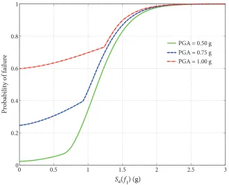
2. When the spectral value at one dimension is fixed at a non-zero value, the probability of failure is not equal to zero even though spectral values of all remaining GMPs approach zero. For a two-dimensional fragility surface, when spectral value at one dimension is fixed at a non-zero value, the probability of failure distribution is a curve representing the probability of failure verses the

GMP at the other dimension. Figure 4 shows the probability of failure of

S

_a

( )

f

₁ when PGA is

fixed at several discrete values.

3. The fragility surface is the combination of discrete points with different lognormal distribution parameters. In the proposed method, a great number of fictitious GRS are defined as seismic input. Recall that ratio factor is dependent on the seismic input. As a result, the points on the fragility surface are lognormally distributed with different lognormal distribution parameters. 4. The proposed method is an extension of seismic FA. It is noticed that, for straight lines radiated

from the origin point of fragility surface, spectral values of GMPs are proportional. Recall that in seismic FA, spectral values within the frequency range are also proportional with the value of a specified GMP. It indicates that the proposed method is an extension of seismic FA. Using a plane in vertical direction to cut the fragility surface can obtain fragility curves with different ratios of GMPs. If the reduction in spectral shape variability is not taken into consideration, the curve from the fragility surface is the same as the fragility curve obtained from seismic FA.

To demonstrate the advantages and applicability of the proposed method, numerical study for a horizontal heat exchanger is conducted in the following section.

Figure 4. Probability of Failure of

S

_a

( )

f

₁ When PGA is Fixed at Discrete Values

NUMERICAL EXAMPLE FOR A HORIZONTAL HEAT EXCHANGER

(8)

Probabilistic Seismic Hazard Analysis (PSHA) for Pickering NPP site is conducted to calculate the

Uniform Hazard Spectrum (UHS) with mean annual frequency of exceedance of 4

×

10-4 (2% in 50

years), as shown in Figure 5.

Figure 5. UHS for Mean Annual Frequency of Exceedance 4

×

10-4at Pickering NPP Site

Since the longitudinal mode is dominant in seismic demand of the heat exchanger, spectral acceleration

L

(

)

a

S

f

in longitudinal direction and PGA are used as GMPs. Spectral acceleration in transverse

direction

S

_a

(

f

_T

)

is assumed to be proportional with PGA in the fictitious GRS. The ratio of

S

_a

(

f

_T

)

and

PGA is obtained from the calculated UHS in Figure 5. The fragility surface of the heat exchanger using two GMPs can be determined in accordance with the procedure presented previously.

The probability of failure histogram of the heat exchanger is shown in Figure 6. The fragility surface can be approximated by the histogram as long as the size of maximum discrete interval is sufficient small. It can be seen that the probability of failure distribution is a two-dimensional fragility surface instead of a curve. It can better predict the failure of individual SSC induced by potential earthquakes with different

combinations of spectral values of

S

_a

(

f

_L

)

and PGA.

When the ratio of

S

_a

(

f

_L

)

and PGA is equal to that of NUREG/CR-0098 median spectrum, the fragility

surface falls into a curve, as shown in Figure 7. Similarly, one can also obtain another curve with a ratio

of

S

_a

(

f

_L

)

and PGA equal to that of calculated UHS. The results show that fragility curves from the

(9)

Figure 6. Probability of Failure Histogram of

S

_a

(

f

_L

)

and PGA

(10)

CONCLUSIONS

In this paper, a method for predicting fragility surface of individual SSC using multiple GMPs is proposed. In this method, a great number of response spectra corresponding to possible earthquake scenarios induced by potential seismic sources are used as seismic input. Structural dynamic analyses and direct spectrum-to-spectrum method instead of time history analyses are used to calculate structural response of individual SSC. To illustrate the advantages of the proposed method, numerical example for a horizontal heat exchanger is conducted using both seismic FA and proposed methods. The results show that the fragility surface can better describe the seismic capacity of the heat exchanger and reduce the variability in seismic capacity calculation.

REFERENCES

Atkinson, G.M. and Elgohary M. (2007). “Typical Uniform Hazard Spectra for Eastern North America

Sites at Low Probability Levels,” Canadian Journal of Civil Engineering, NRC Research Press,

Canada, 34(1) 12-18.

Baker, J.W. and Cornell, C.A. (2005). “Vector-valued Ground Motion Intensity Measures for

Probabilistic Seismic Demand Analysis,” 13thWorld Conference on Earthquake Engineering,

Vancouver, B.C., Canada.

Bazzurro, P. and Cornell, C.A. (2002). “Vector-valued Probabilistic Seismic Hazard Analysis (VPSHA),”

Proc. of 7thU.S. National Conference on Earthquake Engineering, Boston, Massachusetts, USA.

Chopra, A.K. (2012). Dynamics of Structures: Theory and Applications to Earthquake Engineering, 4th

ed., Pearson Education Inc..

EPRI (1994). “Methodology for Developing Seismic Fragilities, TR-103959,” Electric Power Research Insititue, CA.

Jiang, W., Li, B., Xie, W. C., and Pandey, M.D. (2015). “Generate floor response spectra, part 1: Direct

spectra-to-spectra method (accepted),”Nuclear Engineering and Design,UK.

Kennedy, R. P. and Ravindra, M.K. (1984). “Seismic Fragilities for Nuclear Power Plant Risk Studies,” Nuclear Engineering and Design, 79, 47-68.

Li, B., Jiang, W., Xie, W. C., and Pandey, M. D. (2015). “Generate floor response spectra, part 2: Direct