On the distribution of the mean and variance of a quantitative trait under mutation-selection-drift balance.

(1)

On the Distribution

of the Mean

and

Variance

of

a Quantitative

Trait

Under Mutation-Selection-Drift Balance

Reinhard

Biirger*

and Russell Landet

*Znstitut f u r Mathematik, Uniuersitat Wien, A-1090 Wien, Austria, and 'Department of Biology, University of Oregon, Eugene, Oregon 97403

Manuscript received February 14, 1994 Accepted for publication July 21, 1994

ABSTRACT

The distributions of the mean phenotype and of the genetic variance of a polygenic trait under a balance between mutation, stabilizing selection and genetic drift are investigated. This is done by stochastic simu- lations in which each individual and each gene are represented. The results are compared with theoretical predictions. Some aspects of the existing theories for the evolution of quantitative traits are discussed. The maintenance of genetic variance and the average dynamics of phenotypic evolution in finite populations (with Ne < 1000) are generally simpler than those suggested by some recent deterministic theories for infinite populations.

T

HE importance of polygenic mutations for the maintenance of genetic variation in quantitative traits and for the response to long-term directional selection has been investigated and discussed in numerous publications (e.g., LANDE 1975,1988; HILL 1982; TURELLI

1984; LYNCH and HILL 1986; KEIGHTLEY and HILL 1983, 1988; SLATKIN 1987; BURGER et al. 1989; HOULE 1989) [cf. BULMER (1989) and BARTON and TURELLI (1989) for re- views and further references]. There seems to be some consensus that mutation can contribute substantially to the maintenance of genetic variation although the extent may differ greatly between species and traits. Many other mechanisms and models have been suggested or

investigated that either reduce or increase the amount of heritable variation compared to the simple mutation- selection-balance hypothesis. As a consequence of the well known disputes about this subject, fresh experimen- talapproaches have been started ( e . g . , CABALLERO et al.

1991; MACKAYet al. 1992; SANTIAGO et al. 1992; LOPEZ and LOPEZ-FANJUL 1993a,b).

Many of the theoretical analyses have been devoted to deterministic models, ignoring the consequences of genetic drift in finite populations, and considerable progress in the understanding of such multilocus models has been achieved (LATTER 1960; &MUM 1965;

BULMER 1972; LANDE 1975; FLEMING 1979; TURELLI 1984;

BARTON 1986; BARTON and TURELLI 1987; SLATKIN

1987; BURGER 1989; FRANK and SLATKIN 1990; HASTINGS

1990; TURELLI and BARTON 1990; B ~ R G E R and HOFBAUER

1994; to mention just a few). However, the overall conclusion that must be drawn from these investigations, and this was particularly stressed by TURELLI and BARTON

(1990), is that the evolutionary dynamics of quantitative traits crucially depends on so many assumptions and genetic details that it is unlikely that general, simple, and reliable predictions can ever be made.

Genetics 138: 901-912 (November, 1994)

In this study, we investigate the distribution of the mean phenotype and of the genetic variance of a quantitative character under mutation-stabilizing selection balance in a finite population. We compare the simulation results with the phenotypic theory for the mean phenotype Of LANDE (1976) and with predictions for the distribution of the genetic variance by LYNCH and HILL

(1986), BARTON (1989) and BURGER et al. (1989). On the basis of these and other results, we conclude that several of the complications occurring in deterministic polygenic models are simplified by genetic drift and thus are of much less importance in small or moderately large populations.

THEORY

We give a brief summary of those theoretical results on the distribution of a quantitative trait in a finite population whose validity will be investigated in the next section. We consider a randomly mating, finite population of constant effective size Ne with discrete generations. Individual fitness is determined by a single quantitative character under Gaussian stabilizing selection on viability, with the optimum phenotype at zero, Le., the viability of an individual with phenotypic value z is assumed to be

where o2 is inversely proportional to the strength of stabilizing selection.

The quantitative character under consideration is as-

(2)

902 R. Biirger and R. Lande

the genetic contribution and a normally distributed environmental effect with mean zero and variance a: = 1. Therefore, the phenotypic mean 5 equals the mean of the additive genetic values, g, and the phenotypic variance is u: = ai

+

uf , with ui denoting the

(additive) genetic variance. We shall use the parameter

V ,

= w 2

+

af = w 2

+

1 to describe the strength of stabilizing selection on the breeding values.

Distribution of the mean phenotype: Random sampling in a finite population induces stochasticity in the evolution of the mean phenotype and, more generally, of the whole distribution of phenotypic values. There- fore, a proper understanding of phenotypic evolution requires the knowledge of the sampling distribution of the average phenotype, of the genetic (and hence phenotypic) variance, etc. Under the empirically testable assumption of a normal distribution of phenotypic values, LANDE (1976) showed that the distribution of the average phenotype is normal under stabilizing selection as in ( 1 ) . In particular, he derived the dynamics of the expected mean phenotype and of its variance. At stochastic equilibrium, the expected mean phenotype o b viously coincides with the optimum phenotype zero, and LANDE'S (1976) formula (17b) yields the variance of the distribution of Z, i e . ,

V(2) = (6;

+

v,)2 af Ne(&;

+

2V,)

+-

BN,

where 6; denotes the average genetic variance at equilibrium, and the second term in (2a) accounts for mea- suring the phenotype among a finite number BN of progeny before selection ( B the birth rate; see below). LANDE'S theory for the distribution of the mean phenotype does not depend on specific mechanisms determin- ing how genetic variation is maintained under stabilizing selection and random drift. It depends on the assumption that selection acts only on the phenotype, and that nothing other than selection and drift affect the mean phenotype.

Distribution of the genetic variance: To obtain approximations for the distribution of the genetic variance, the mechanism by which genetic variability is maintained must be specified. We assume that it is through mutation. Let p denote the mutation rate per haploid locus. Following CROW and &MUM'S (1964) continuum-of-alleles model, we assume an effectively continuous distribution of possible effect for mutants with mean zero, variance a2, and no skewness. There is no restriction on the number of possible alleles per locus.

Various theories and approximations have been derived for the expected value of the additive genetic variance in a finite population under a balance between

selection, mutation, and random genetic drift (see references below).

For a neutral phenotypic character, LYNCH and HILL

(1986) showed that the expected genetic variance under mutationdrift balance is

(2N, - 1)'

6: (N) = V,

2%

-

2Ne V,, (3b)

where V, = 2npa2 is the variance introduced by mutation each generation (see also CLAWON and ROBERTSON 1955). Their model assumes that 4N,p < 1, so that it is unlikely to have more than two alleles per locus.

For stabilizing selection acting on the phenotype according to ( l ) , the approximate formula

6;(SHC) = 4npa2Ne

1

+

(ff2Ne/V,>

for the expected genetic variance has been found in- dependently, by different methods, and almost at the same time by four groups of authors (BURGER 1988;

KEIGHTLEY and HILL 1988; BARTON 1989; BURGER et al.

1989; HOULE 1989). It has been called the stochastic house-of-cards approximation because, in the limit of infinite population size, (4) reduces to TURELLI'S (1984)

so-called house-ofcards (HC) approximation

6i(HC) = 4npV,. (5)

This is identical to the two-allele approximations of LATTER (1960) and BULMER (1972). The generality and accuracy of (5) were investigated recently by BURGER

and HOFBAUER (1994). In the limit of weak selection, i. e., V, + m, (4) reduces to the neutral formula (3b).

The approximation (4) was derived for the continuum-of-alleles model using the HGapproxima- tion (5) and diffusion theory (cf. BURGER et al. 1989),

and it can be rewritten as half the harmonic mean of (3b) and (5), L e . ,

&;(N)~;(Hc) 6i(SHC) =

b i ( N )

+

6i(HC)'

The validity of the SHGapproximation (Equation 4 or

6) requires low mutation rates per locus and a high variance a2 of the distribution of mutant effects because the HC-approximation does so and because the neutral a p proximation requires small p. For high mutation rates or low

CY',

the Gaussian approximation of KIMURA (1965) and its multilocus extension by LANDE (1975) are more appropriate and could be inserted into (6) instead of 6: (HC) (see also LATTER 1970; LYNCH and LANDE 1993). All the formulas in this section are based on the assumption of linkage equilibrium.

Extensive stochastic computer simulations (BURGER

(3)

903

equilibrium variance for a wide range of parameters. KEIGHTLEY and HILL (1988) obtained values of the genetic variance that are up to 30% larger than predicted by (4). The reason is that their transition matrix a p proach, for equal allelic effects across loci being equiva- lent to BULMER’S (1972) model, is based on a deterministic recursion equation with heterozygote disadvantage at each locus. This heterozygote disadvantage is a consequence of the assumption that the gene frequencies are always such that the mean phenotype is at the fitness optimum, which, however, is not satisfied in the full multilocus model. Consideration of the marginal fitness values, as appropriate under the assumption of global linkage equilibrium, shows that each locus is under directional selection and this should lead to a lower genetic variance. BARTON’S (1989) simulation model with

two alleles per locus, is based on the correct deterministic equations for the gene frequency change in the full multilocus model and yields estimates of the genetic variance that are below those of BULMER (1972) and KEIGHTLEY and HILL (1988) but higher than (4). This is not surprising, because in BARTON’S simulation model alleles still occur in pairs, symmetric with respect to the optimum. The present simulations [as those in B~JRGER

et al. (1989) and B ~ R G E R (1989)l neither assume linkage equilibrium, nor equal allelic effects, nor are they based on deterministic recursion equations. It turns out that a better approximation is obtained in the case where random drift is strong compared to selection if in (6) formula (3a) is used for &: (N) instead of (3b).

The distribution of the genetic variance, in particular the variance of the genetic variance,

qui)

has been stud- ied in detail only in the neutral case. Under the assump tion 4Nep < 1, so that the likelihood of more than two segregating alleles per locus is negligible, LYNCH and

HILL (1986) showed that for a normal distribution of mutational effects with mean zero

‘I

-

&;(N)(Y*,

if 4Nep

<<

1 and 2np

<<

1.

ZENC and COCKERHAM (1991), using a different model of mutation with a limited range of allelic effects, obtained (7a) but with +2/n instead of - l / n . For a neutral model without mutation, BULMER (1980, p. 230) calculated the variance of the components of genetic variance that are due to random departures from Hardy- Weinberg equilibrium, Cw, and linkage disequilibrium,

q.

Denoting the “true” variance, which would be observed in Hardy-Weinberg and linkage equilibrium for a given set of gene frequencies, by V, he showed that Var( Cw) = V$/Ne and, in the absence of linkage, Var(Ci) == 5V$/3Ne. Comparison with (7a) shows that

these terms are small provided that 4np

<<

1. LYNCH

and HILL (1986) apparently neglected variation due to Hardy-Weinberg disequilibrium and their term

2&:(N)‘/(3Ne), for variation due to departures from linkage equilibrium, differs from BULMERS by a factor 5/2. AWRY and HILL (1977) obtained 4V$/(3Ne) for that quantity. Our formula (A.27) for the variance of the genetic variance agrees, to first order, with (7b) if 4Nep

<<

1 and if the mutant distribution is normal.

For phenotypic characters under stabilizing selection, the variance of the genetic variance can be approximated by

&.2,(SHC)a2 = 1

+

(a2Ne/V,)

(BARTON 1989). In the limit of V, + m, this reduces to (7b). Higher moments of the distribution of the genetic variance seem to be unknown.

METHODS AND RESULTS

The theoretical results about the distribution of the mean phenotype and the genetic variance are based on various simplifjmg assumptions. This is unavoidable because of the notorious difficulties encountered in the analysis of polygenic models. Therefore, we have performed comprehensive stochastic computer simulations to check these approximations.

The simulation model: This has been adapted from the one used in BURGER et al. (1989) and BURGER and

LYNCH (1994). It uses direct Monte-Carlo simulation, representing each individual and each gene. The genotypic value of the character is determined by n additive loci with no dominance or epistasis. We chose n = 50 for all of our simulations. We simulate the continuum-of- alleles model of CROW and KIMURA (1964) by drawing individual allelic effects from a continuous distribution, so the number of possible segregating alleles per locus is limited only by population size. The phenotypic value of an individual is obtained from the genotypic value by adding a random number drawn from a normal distribution with mean zero and variance a: = 1. The generations are discrete, and the life cycle consists of three stages: (a) random sampling of breeding pairs from the surviving offspring of the preceding generation, (b) pro- duction of offspring, including mutation and recombination, (c) viability selection according to (1).

Each breeding pair produces exactly 2B offspring and, for all parameter values shown below, more than

90% of these survive viability selection. Random sampling of N parents is performed without replacement and the sex-ratio is 1:l. Thus, the number of breeding adults is always N and the mating system is dioecious and monogamous. The effective population size is Ne =

4N/(V,

+

2), where V, = 2(1 - l / B ) [ l - (2B - 1)/

( B N - l ) ] is the variance in family size. For further details see BURGER et al. (1989) and BURGER and LYNCH

(4)

904 R. Burger and R. Lande

TABLE 1

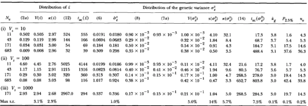
The distribution of the mean phenotype Z and of the genetic variance a: under mutationaelection-drift balance

Distribution of i Distribution of the genetic variance a:

Ne ( 2 a ) V ( i ) K ( Z ) (12) t a c ( i ) (6) &f (8) (7a) Wu:) s ( u 3 4 ~ : ) (14) &(ai) kg P2.5% ae

(i) V, = 10

11 0.502 0.505 2.97 524 555 0.0191 0.0180 0.90 X 0.93 X 1.00 X lop3 4.10 32.1 43 0.129 0.119 2.99 144 166 0.0694 0.0683 0.29 X lo-' 0.32 X 106' 1.84 8.4

171 0.034 0.031 3.00 54 69 0.184 0.181 0.50 X lo-' 0.54 X lo-' 0.91 4.3 683 0.009 0.008 2.96 32 39 0.309 0.298 0.35 X 106'

17.3 3.8 1.6 4.3 68.7 3.7 5.4 5.3 184.7 3.1 17.5 14.6 0.38 X lo-' 0.50 3.5 488.4 3.1 37.6 36.3 (ii) V, = 100

11 4.60 4.45 2.76 5025 4144 0.0199 0.0186 0.99 X lop3 0.93 X 0.11 X 106' 4.11 32.4 21.6 17.2 3.8 1.7 4.0 43 1.17 1.15 2.91 1215 1316 0.0823 0.0814 0.40 X lo-' 0.41 X lo-' 0.46 X 106' 1.94 9.6 80.5 76.7 3.6 5.7 5.3 171 0.29 0.30 3.02 320 360 0.313 0.307 0.14 X 10-1 0.15 X 10-1 0.17 X 106' 1.00 4.7 268.5 278.0 3.0 19.4 14.3

683 0.08 0.08 3.03 98 116 1.017 0.924 0.38 X lo-' 0.42 X 10" 0.47 3.3 652.7 803.8 3.0 42.4 33.8 (iii) V, = 1000

171 2.93 2.94 2.68 2967.0 294 0.337 0.336 0.17 X 10-1 0.15 X 10-1 0.21 X 106' 1.04 5.0 268.5 284.3 3.0 19.7 14.3 Max S.E. 3.1% 2.3% 1.0% 5.0% 14% 5.7% 7.5% 0.1% 0.1% 0.2%

The symbols V ( . ) , s(.), and K ( . ) refer to the variance, the skewness, and the kurtosis, respectively. Also shown are the autocorrelation time for

the mean phenotype, t,, ( i ) , the autocorrelation time of the genetic variance, tac(ai), the average kurtosis k of genotypic values, the average number of polymorphic loci, P2.596, on a 2.5% level, and the effective number ne of segregating loci. Theoretical values are indicated by their equation number and compared to observed values from the simulation (see text). For all parameter combinations in this table, the mutant distribution is Gaussian with variance cy2 = 0.05 and the mutation rate per haploid locus is p = 0.0002. This gives a genomic mutation rate of

2 n p = 0.02 and a mutational variance per generation of V,/a; = as approximately observed in empirical studies (LANDE 1975; LYNCH 1988). There is free recombination between all loci. The bottom row contains the maximum standard error in percent of the mean of the data in the

g

corresponding column.

In our simulations, we chose four different population sizes, i.e., N = 8, 32, 128, and 512 breeding adults. For all these population sizes, we chose B = 2. This leads to effective population sizes of Ne = 11,43,171, and 683, respectively. The observed Ne's in our simulations differ from these by less than 1 % , for large N by less than 0.1 %

.

(The effective population size has been calculated by storing for each offspring the (indices of the) parents it came from, and then calculating the variance of family size among the offspring that survived selection.) For each parameter combination, a certain number of r e p licate runs with stochastically independent initial populations were performed, each run over lo5 generations. Initial populations were obtained from a preceding initial phase of several hundreds or thousands of generations (depending on N ) during which mutation- selection balance had been reached. The number of replicate runs per parameter combination was 100, 40, 25, and 10 for N = 8,32,128,512, resp. This yieldedvery small standard errors (see below), much smaller than in earlier simulations.

The distribution of the mean phenotype and of the genetic variance: The present simulations show, con- firming a trend suggested by the simulation results in

BURGER et al. (1989) and BURGER (1989) that the SHC-

approximation (4) tends to overestimate the true equilibrium variance, in particular when genetic drift pre- vails. One of the reasons is that (3b) overestimates the neutral variance &;(N) for small Ne. Also the H G approximation overestimates the true equilibrium variance in infinite populations (cf. BURGER and HOFBAUER

1994). Therefore, all theoretical results below are based

on choosing (6) in conjunction with (3a) as analytical approximation for the genetic variance. For the variance of the mean phenotype V(Z), Equation 2a in conjunction with (6) is used. Results for the distribution of the mean phenotype and the genetic variance are summa- rized in Tables 1 and 2. Previous simulations (BURGER

et al. 1989) have shown, as suggested by formulas (3) and (4), that the average genetic variance depends in a linear way on the genomic mutation rate 2np and not on p and n separately, if the loci are unlinked and n is not too small (say n 2 10). Equations 2,7, and 8 suggest

that this remains true for the variance of the mean phenotype and of the genetic variance but we have not checked this by simulation.

The statistics displayed in Table 1 show that the distribution of the mean phenotype is almost perfectly Gaussian (a Gaussian distribution has a kurtosis of K = m4/u4 = 3.0) and LANDE'S (1976) formula for the variance of the mean phenotype (Equation 2) is very accurate. Only for weak selection, i e . , small Ne/V,, is the distribution of the mean slightly platykurtic. This Gaus- sian theory also works well for other mutation parameters and mutant distributions, and also for linked loci (see Table 2). In contrast to our results, BARTON (1989) had found that the variance of the mean phenotype is lower than predicted by (2b) which is even smaller than (2a) and yields V(Z) = 0.0292 for the parameters in Table 2. In his model, however, there are exactly two

alleles with effects ctu at each locus. This may lead to multiple stable equilibria, and the mean phenotype does not necessarily coincide with the optimum (BARTON

(5)

Quantitative Dynamics

TABLE 2

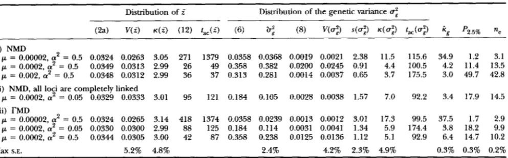
Continuation of the distribution of the mean phenotype i and of the genetic variance u: under mutation-selectiondrift balance

Distribution o f f Distribution of the genetic variance u:

(i) NMD

p = 0.00002, 'a = 0.5 0.0324 0.0263 3.05 271 1379 0.0358 0.0368 0.0019 0.0021 2.38 11.5 115.6 34.9 1.2 3.1

p = 0.0002, a2 = 0.5 0.0349 0.0313 2.99 26 49 0.358 0.382 0.0200 0.0245 0.91 4.4 100.5 4.2 11.4 13.5

p = 0.002, 'a = 0.5 0.0348 0.0312 2.99 36 37 0.313 0.281 0.0014 0.0037 0.65 3.7 175.5 3.0 49.7 42.8 (ii) NMD, all loci are completely linked

p = 0.0002, 'a = 0.05 0.0329 0.0333 3.01 95 121 0.184 0.105 0.0028 0.0038 1.57 7.0 92.2 3.4 17.9 14.5 (iii) TMD

p = 0.00002, 'a = 0.5 0.0324 0.0265 3.14 418 1374 0.0358 0.0239 0.0013 0.0012 3.01 17.3 99.5 37.5 1.7 2.9

p = 0.0002, 'a = 0.05 0.0330 0.0300 2.99 88 125 0.184 0.114 0.0031 0.0041 1.34 5.9 174.4 3.8 18.2 9.9

p = 0.0002, a2 = 0.5 0.0344 0.0305 3.00 42 87 0.358 0.238 0.0125 0.0136 1.12 5.1 92.9 6.4 14.7 10.2

Max S.E. 5.2% 4.8% 2.4% 4.2% 2.3% 4.9% 0.3% 0.3% 0.2%

Since, for many of the parameter combinations here, (6) does not give accurate estimates for the equilibrium genetic variance, the values of (2a), (8), and (12) are based on the observed value 6;. In all cases, V, = 10 and Ne = 171. NMD indicates a normal mutant distribution with variance a', TMD a reflected rdistribution with variance a2 and j3 = 0.5. (The latter is defined by As( x i 8-1 exp(-A i x i )/(2r(j3)), where the constants A and fl can be chosen such that this distribution has a predefined variance and kurtosis. For j3 = 0.5, the kurtosis becomes 11.7) (See KEIGHTLEY and HILL 1988; BURGER 1993).

locus continuum-of-alleles model behaves more simply (and likely more realistically) than this biallelic model and always leads to an equilibrium distribution of genotypic values such that the mean phenotype coincides with the optimum if the mutant distribution is symmetric ( c j BURGER and HOFBAUER 1994). This seems to carry over to some extent to the finite population case (see also BARTON 1989) and is most likely the reason for the different results.

Concerning the average genetic variance, Table 1 confirms the finding by BURGER et al. (1989) that the SHGapproximation (Equations 4 or 6) predicts the ob- served genetic variance accurately, although in all cases it gives a slight overestimate. The variance of the genetic variance is well predicted by BARTON'S (1989) formula (our (8)), however, it always underestimates the observed V(a:) by approximately 10%. Calculating (8) on the basis of the observed average variance 6:, leads to a slightly greater underestimate. For the cases where

Ne/ V, <

2,

the approximation (7a), due to LYNCH and HILL (1986), is included. For small Ne and very weak selection, it is even lower than BARTON'S prediction because then (7a) is smaller than (7b) which would cor- respond to (8).

As

observed in BURGER (1989), the SHC- prediction tends to overestimate the observed genetic variance considerably, either if the loci are very tightly linked (so that effectively there is only one locus with a high mutation rate), or if the variance of mutational effects becomes small, or if the mutant distribution is highly leptokurtic. This overestimate is a consequence of the corresponding property of the HGapproximation in the infinite population case (see BURGER and HOFBAUER 1994). Then the approximation (8) for V(ug may become rather inaccurate even if, as in Table

2,

the observed genetic variance 6: instead of (6) is inserted into (8). Nevertheless, the Gaussian approxi-

mation for the distribution of the mean phenotypes remains fairly accurate, unless the genomic mutation rate 2np becomes very low, as for p = 0.00002.

The average genic variance is always slightly larger than the average genetic variance but for the parameter combinations displayed in Table 1, this difference is always less than two percent (results not displayed). This shows that Hardy-Weinberg and linkage disequilibria can safely be ignored unless linkage is tight ( c j LANDE 1975; BURGER 1989; TURELU and BARTON 1990).

(6)

906 R. Riirger and R. Lande

0.50 I I I I

0.45

0.15

'

I I I I

0 1000 2000 3000 4000 5000

5.0 1 I I I I

.z? 4.5

d I t I

1 - 1

2.5 I ""~~ I

0 1000 2000 3000 4000 5000

Generations

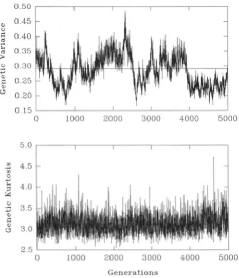
FIGURE 1 .-Evolution of genetic variance (upper panel) and genetic kurtosis (lower panel) under mutation-selection-drift

balance in one run with the following parameters: N , = 683,

V,

= 10, 50 loci, p = 0.0002, normal mutant distribution with variance a* = 0.05. The straight lines represent the average genetic variance (= 0.285) and the average genetic kurtosis (= 3.12) for this run (compare Table 1, (i), line 4). The medians of the distributions of genetic variance and genetic kurtosis are 0.284 and 3.10, respectively.

nearly Gaussian most of the time with occasional ex- cursions that may be dramatic if mutational effects are large.

Autocorrelation of the mean phenotype and the genetic variance: The simulations show high fluctuations of the mean, variance, etc., between generations and substantial autocorrelation. This has been noticed earlier by KEICHTLEY and HILL (1983) for directional selection and by KEICHTLEY and HILL (1988) and BURGER

et al. (1989) for stabilizing selection. Figures 1 and 2 display the extent of this phenomenon.

In the present investigation, we have measured these autocorrelations as follows. Denote by X( t ) the value of a random variable ( e . g . , the genetic variance) in generation t . Then the autocorrelation function is

Cov[X(t), X(t

+

41

( P ( 4 = (9)

vVar[X(t)JVar[X(t

+

T)]

.

In our simulations, t ran from 1 to IO', whereas the autocorrelation function was calculated only for T between

1 and 5 X lo4, so that the values for the Cov[X(t), X( t

+

T)] are based on at least 5 X lo4 data points. We found that the function ( ~ ( 7 ) declines exponentially and

then fluctuates around zero for large 7. Using a least

squares method, an exponential function e P r was fit-

0.9

,

I I I I _I

0.8

0.7

.: 0.6

2

0.5 v 0.4

r, 0.3

0 0.2

0.1

-

.-

2

u

0 . 0 L

0 1000 2000 3000 4000 5000

7 0 'g 60

2

50

u)

r)

x ₄₀

5

30

$ 20 u

10

0 I O 0 0 2000 3000 '1000 5000

Generations

FIGURE 2.-& Figure 1, but with the following parameters: N, = 171, V, = 10, 50 loci, p = 0.0002, reflected

r

mutant distribution with variance a* = 0.5. The average genetic variance and the average genetic kurtosis for this run are 0.233 and 6.27, respectively (compare Table 2, (iii), line 3). The corresponding medians are 0.213 and 4.83.

ted to ( ~ ( 7 ) such that

x:zifl

((~(7)

-

is minimized.

The reciprocal of the unique solution yc is called the characteristic autocorrelation time and denoted by

1

Y c

t,, =

-

.

Different methods, like performing the least squares approximation with weights, yielded similar results. The data (Tables 1, 2) provide quantitative estimates for the importance of the autocorrelation of the mean phenotype and the genetic variance and confirm previous qualitative observations.

An approximation for the autocorrelation function of the mean phenotype can be obtained from LANDE'S (1976) analysis of genetic drift and stabilizing selection. Under weak selection ( V ,

>>

1) and the assumption of a constant genetic variance, he identified the corresponding stochastic process as an Ornstein-Uhlenbeck diffusion process for the mean phenotype with infini- tesimal mean &:/(

V,

+

6:) and variance &:/Nc. This has autocorrelation function

(7)

autocorrelation time is

This result does not depend explicitly on Ne and gives a rather good approximation to the observed values as long as the coefficient of variation of a: is small ( CJ Tables 1 and 2).

We have shown for a neutral model, assuming two segregating alleles per locus, i. e., 4Nep

<<

1, and global linkage equilibrium, that the autocorrelation function for the genetic variance is given by

so that the autocorrelation time is

(see APPENDIX). BULMER (1980, p. 230) showed that random departures from Hardy-Weinberg equilibrium cause uncorrelated fluctuations of the genetic variance and, in the absence of linkage, random departures from linkage disequilibrium lead to a correlation of 1/2 between successive values of genetic variance. The first gives an autocomelation time of zero whereas the latter gives a value of two, which is small compared to (14) ( cf.

also AWRY and HILL 1977). For weak selection and 4Nep

<<

1, theory and data are in reasonably good agree- ment ( cf. Table 1).

We have also measured the autocorrelation time of the genetic kurtosis. It tends to be slightly larger than that of the genetic variance (results not shown).

The effective number of segregating factors: In the present model, the number of segregating loci is always smaller than the number of all loci potentially contrib uting to the trait. We calculated the effective number ne

of loci according to LANDE’S (1981) formula

where a, is the standard deviation of the distribution of

allelic effects at one (haploid) locus, and the expectation is taken over all loci at male and female gametes. Data are displayed in Tables 1 and 2. If the number of

effective loci i s sufficiently high, in our simulations approximately ne 2 15, the distribution of breeding values

is nearly Gaussian. In addition, we compared ne to the average polymorphism P2,5% on a 2.5% level. The crite- rion in our simulations for a locus to be polymorphic was that there were more than 5% heterozygotes at a locus which implies that the most frequent allele has a frequency of less than 97.5%.

Directional selection: It would be desirable to have a theory for the distribution of the mean phenotype and

the genetic variance under directional selection. Such a theory is not currently available. Following LYNCH and

LANDE (1993) and BCIRGER and LYNCH (1994), we modeled directional selection by a “moving optimum,” i.e., by

Yt

= exp

{-

T } ,

(Z

-

kt)2

where k is a positive constant describing the rate at which the optimum phenotype moves. For k low enough (below a critical rate of environmental change, c$ LYNCH and L W D E 1993; BCIRGER and LYNCH 1994), populations prac- tically persist for ever. For this kind of directional selection, the variances of the mean phenotype and of the genetic variance have a major influence on the dynamics of evolution and extinction (BCIRGER and LYNCH 1994).

Extending these investigations, we performed several simulations for a slowly moving optimum, i . e., k so small that the average mean fitness was still higher than 0.85,

compared to 0.95 for pure stabilizing selection with w2 = 9. Thus the number of breeding adults and the effective populations size remained constant during the lo5 generations, each simulation run lasted.

As

shown by LYNCH and LANDE (1993), a steady-state distribution builds up that responds constantly to directional selection but the mean phenotype lags behind the optimum. For this “traveling wave,” we found (results not shown) that even a very low k , i . e . , k

-

4% of a phenotypic standard deviation of an i n i t i a l population, leads to a more than twofold increase of 6;, to a sixfold increase of V(ai), to a 3.5-fold increase of V ( i ) , and to a decrease of tac by a factor 1/6, as compared to the initial equilibrium distribution (with k = 0 ) . Further increasing k

leads to a further increase of 6:, V(a:), and V ( f ) , and to a further decrease of

tat.

The genetic variance

e:,

however, levels off soon (see also BCJRGER and LYNCH 1994) and always remains below the neutral prediction (3).

DISCUSSION AND CONCLUSIONS

For many evolutionary biologists and geneticists, the only simple conclusion emerging from the last decade of theoretical investigations on the dynamics of quantitative-genetic variance and the dynamics of phenotypic evolution might be that the theories are often excessively complicated and frequently depend on a plethora of parameters that are difficult or impossible to measure. We would like to summarize below a few simple and useful results that have emerged from our simulations and other recent studies.

The majority of the theoretical studies dealt with infinite populations, i . e . , they neglected random drift, It turned out that many results depend strongly on details of the assumptions. For example, under stabilizing selection the Gaussian theory of &Mum (1965) and LWDE

(8)

908 R. Biirger and R Lande

reason for the discrepancy between these approximations is that they are based on different assumptions about the mutation parameters, ie., they are valid in different regions of the parameter space. Both approximations can be mathematically justified, and both a p proximations always overestimate the true equilibrium variance (BURGER and HOFBAUER 1994). As is well known, TURELLI (1984) and BARTON and TURELLI (1989) have argued that current empirical knowledge suggests parameter values in favor of the HGapproximation to be the more plausible ones.

We based many of our simulations on such parameters estimates [ c$ also LANDE (1975) and LYNCH (1988)l. In addition, we investigated how the shape of the mutant distribution affects the equilibrium distribution of the trait because theoretical arguments (KEIGHTLEYand HILL

1988) as well as recent empirical results ( e . g . , MACKAY

et al. 1992) indicate that mutant distributions may be highly leptokurtic. This means that most new mutational variance is due to few mutants with large effects whereas the majority of mutants has very little or no effect. The present simulations show, and for infinite populations this was mathematically proved by BCJRGER and HOFBAUER

(1994), that increasing the kurtosis of the mutant distribution leads to increasing deviations from the SHC- approximation (see Tables 1 and 2). Ironically, given that all other parameters are the same, Gaussian mutant distributions are more favourable to TURELLI’S (1984)

HC-approximation (or rare-alleles approximation) than mutant distributions dominated by rare alleles with large effects.

It is important to notice that genetic drift in finite populations reduces the discrepancy between the Gaus- sian and the HC-approximation, as encompassed in deterministic models. In finite populations, the genetic variance is always below that predicted by the neutral mutationdrift balance (LYNCH and HILL 1986) and, in small populations, it is always very close to it. In fact, for small population size or weak selection, the SHG prediction (6) and the stochastic version of the Gaussian approximation ( cf. LATER 1970; LYNCH and LANDE 1993)

deviate only slightly, because both are close to the neutral prediction. The present simulations confirm earlier results (BURGER et al. 1989) that the SHGprediction is a very good approximation for a reasonably wide range of parameters. However, in most cases it is an overestimate. Our results also show that BARTON’S (1989) theory for the variance of the genetic variance (8) provides good estimates as long as the SHC-approximation applies.

In deterministic multilocus models the situation is

much more complicated. For example, BARTON (1986)

showed that many simultaneously stable equilibria, giving rise to different levels of genetic variance and to mean phenotypes deviating from the optimum, may ex- ist. On the other hand, a deterministic multilocus model allowing for a continuum of possible alleles at each lo-

cus, yields much simpler results: the mean phenotype is always very close to the optimum (and agrees with the optimum if the mutant distributions are symmetric) and, for small mutation rates or large variance of mutational effects, the equilibrium genetic variance is closely approximated by the HC-prediction (cf. B~JRGER and HOFBAUER 1994).

Although our simulations are based on the continuum-of-alleles model, the number of actually segregating alleles per locus typically is small. Depending on the parameters, for any given point in time, a considerable fraction of loci even is monomorphic (see Tables 1 and 2 for the average polymorphism and the effective number of factors), and at the other loci two or

(sometimes) more alleles segregate. This is certainly more realistic than the above deterministic models, and also more realistic than stochastic models based on diallelic loci with symmetric effects, as in BULMER (1972),

KEIGHTLEY and HILL (1988) and Barton (1989). Never- theless, in contrast to the deterministic models, all these stochastic models, including the simulations of HOULE

(1989) of a model with three alleles per locus and that of FOLEY (1992), yield qualitatively similar results in many respects, though they differ quantitatively to a moderate extent.

The present simulations show that in finite populations the mean phenotype indeed behaves extremely simply, at least on the average. Its distribution is almost perfectly Gaussian, as predicted by LANDE’S (1976) phenotypic theory, and the variance of the mean phenotype agrees closely with the phenotypic prediction V,/2Ne

(2), unless the variance of mutational effects is very large and the (genomic) mutation rate very low. This, together with the fact that the genetic variance is almost always less than or equal to the SHGapproximation, suggests that multiple stable equilibria are of little relevance in populations of small and moderate effective size.

One potentially cumbersome problem investigated and quantified by the present simulations and theory is the high autocorrelation of the genetic variance and other quantities (like mean phenotype, mean fitness, genic variance, genetic kurtosis). This was already noticed previously (KEIGHTLEY and HILL 1988; BURGER et al.

(9)

Quantitative Dynamics

These high autocorrelations pose serious problems for conclusions based on measurements of genetic variance because of the long-lasting influence of random excur- sions of the variance.

Under directional selection according to a moving op- timum (16), the autocorrelation of the genetic variance becomes much smaller. On the other hand, the variance of the mean phenotype and of the genetic variance may be an order of magnitude larger than under stabilizing selection of the same strength. Also the genetic variance increases under this form of selection and approaches a steady-state value which is higher than the SHC- prediction but lower than the neutral prediction ( CJ

BURGER and LYNCH 1994). The latter has been shown to be the asymptotic variance under both truncation selection (HILL 1982) as well as under exponential directional selection (BURGER 1993). In the latter case, a simple Gaussian approximation yields correct predictions for the evolution of the mean phenotype and of the genetic variance. This is not the case for a moving op- timum, where the Gaussian approximation gives an approximately correct theory only for the evolution of the mean phenotype but always underestimates the lag between the optimum and the mean (cf. LYNCH and LANDE

1993; B ~ R G E R and LYNCH 1994). Nevertheless, in all these cases the distribution of the breeding values is approximately Gaussian unless selection becomes very strong. No satisfjmg theory for the distribution of the mean phenotype or the genetic variance is available for a moving optimum. Finite populations of small or moderate size (say Ne < 500) also behave more reasonably in response to directional selection than predicted from deterministic theory (BARTON and TURELLI 1987). Neither under exponential directional selection nor under a moving optimum is a substantial increase of genetic variance observed unless previous stabilizing selection was extremely strong (cf. B ~ R G E R 1993; B ~ R G E R and LYNCH

1994). The reason is that for such population sizes the equilibrium variance under stabilizing selection, which is approximately given by the SHC-prediction, is not much lower than the neutral prediction which appears to pose an upper limit to the genetic variance under most forms of directional selection.

To summarize, there are a number of issues that are simplified by having small population size. Among these are that (i) multiple equilibria apparently are of little relevance as suggested by the accuracy of the Gaussian theory for the mean phenotype (compare also BARTON

1989); (ii) for small populations, the stochastic ana- logues of the Gaussian and the house-ofcards approximation for the genetic variance do not differ very much because both are close to the neutral prediction. The stochastic house-ofcards prediction yields a good approximation; (iii) if a finite population under mutation- selectiondrift balance is exposed to directional selection, a large increase of genetic variance, as predicted by the deterministic theory (BARTON and TURELLI, 1987) but

usually not observed in experiments, does not occur unless the population size is very large or stabilizing selection was very strong (BURGER 1993; BURGER and LYNCH

1994; cf. also KEIGHTLEY and HILL 1989).

The general conclusion that we would like to draw from the present results and those discussed above- though with appropriate caution-is that the maintenance of genetic variance and the dynamics of phenotypic evolution appear to be simpler in finite populations of small or moderate size, compared to the corresponding dynamics in infinite populations when many details of the genetics play an important role. However, due to the stochastic nature of mutation, recombination, and selection, any single population may considerably deviate from that expected behavior of the average population.

The work was partially supported by a research exchange grant from the Max Kade Foundation to R.B., and by National Institutes of Health grant GM27120 to R.L. Numerical simulations were performed on the IBM ES/9021-720 mainframe of the EDV-Zentrum der Universitit Wien. Generous supply with computing time is gratefully acknowledged. We thank the reviewers for their comments.

LITERATURE CITED

AWRY, P. J., and W. G. HILL, 1977 Variability in genetic parameters among small populations. Genet. Res. 2 9 193-213.

BARTON, N. H., 1986 The maintenance of polygenic variation through a balance between mutation and stabilizing selection. Genet. Res. 47: 209-216.

BARTON, N. H., 1989 Divergence of a polygenic system subject

to stabilizing selection, mutation and drift. Genet. Res. 54:

59-77.

BARTON, N. H., and M. Tu-, 1987 Adaptive landscapes, genetic distance and the evolution of quantitative characters. Genet. Res. BARTON, N. H., and M. TURELLI, 1989 Evolutionary quantitative genetics: how little do we know? Annu. Rev. Genet. 23: 337-370.

BULMER, M. G., 1972 The genetic variability of polygenic characters under optimizing selection, mutation and drift. Genet. Res. 19:

BULMER, M. G., 1980 The Mathematical Theory of Quantitative

Genetics. Clarendon Press, Oxford, U.K.

BULMER, M. G., 1989 Maintenance of genetic variability by mutation- selection balance: a child’sguide through thejungle. Genome 31:

BURGER, R., 1988 Mutation-selection balance and continuum-of- alleles models. Math. Biosci. 91: 67-83.

BURGER, R., 1989 Linkage and the maintenance of heritable variation by mutation-selection balance. Genetics 121: 175-184.

BURGER, R., 1993 Predictions of the dynamics of a polygenic character under directional selection. J. Theor. Biol. 162:

487-513.

BURGER, R., and J. HOFBAUER, 1994 Mutation load and mutation- selection balance in quantitative genetic traits. J. Math. Biol. 32:

193-218.

BI~RGER, R, and M. Lwm, 1994 Evolution and extinction in a changing environment: a quantitativegenetic analysis. Evolution (in press). BURGER, R., G. P. WAGNER, and F. STETTINGER, 1989 How much heri-

table variation can be maintained in finite populations by a mutation-selection balance? Evolution 45: 1748-1766.

CABWERO, A., M. A. TORO, and C. LOPEZ-FANJUL, 1991 The response to artificial selection from new mutations in Drosophila melano-

gaster. Genetics 127: 89-102.

CLAYTON, G. A., and A. ROBERTSON, 1955 Mutation and quantitative variation. Am. Nat. 89: 151-158.

COX, D. R., and H. D. MILLER, 1965 The Theory of Stochastic

Processes. Methuen, London.

49: 157-173.

17-25.

(10)

910 R. Biirger and R. Lande

CROW, J. F., and M. KIMuRA, 1964 The theory of genetic loads, pp.

495-505 in Proceedings of the X I International Congress o j

Genetics, edited by S. J. GEERTS. Pergamon, Oxford, U.K.

CROW, J. F., and M. KIMURA, 1970 A n Introduction to Population

Genetics TheoTy. Harper & Row, New York.

FLEMING, W. H., 1979 Equilibrium distributions of continuous polygenic traits. SIAM J. Appl. Math. 36: 148-168.

FOLEY, P., 1992 Small population genetic variability at loci under stabilizing selection. Evolution 64: 763-774.

FRANK, S. A., and M. SLATKIN, 1990 The distribution of allelic effects under mutation and selection. Genet. Res. 55: 111-117.

GARDINER, C. W., 1983 Handbook of Stochastic Methods. Springer- Verlag, New York.

~ I N G S , A., 1990 Maintenance of polygenic variation through mutation-selection balance: bifurcation analysis of a biallelic model. J. Math. Biol. 2 8 329-340.

HILL, W. G., 1982 Rates of change in quantitative traits from fixation of new mutations. Proc. Natl. Acad. Sci. USA 7 9 142-145. HOULE, D., 1989 The maintenance of polygenic variation in finite

populations. Evolution 4 3 1767-1780.

&x-, P. D., and W. G. H n , 1983 Effects of hnlcage on response to directional selection fiom new mutations. Genet Res. 42: 193-206.

KEIGHTLEY, P. D., and W. G. HILL, 1988 Quantitative genetic variation maintained by mutation-stabilizing selection balance in finite populations. Genet. Res. 59: 33-43.

KEIGHTLEY, P. D., and W. G. HILL, 1989 Quantitative geneticvariability maintained by mutation+abilizing selection balance: sampling variation and response to subsequent directional selection. Genet. Res. 54: 45-57.

KIMURA, M, 1965 A stochastic model concerning the maintenance of genetic variability in quantitative characters. Proc. Natl. Acad. Sci. KIMURA, M., and T. OHTA, 1969 The average number of generations

763-771.

until fixation of a mutant gene in a finite population. Genetics 61:

LANDE, R, 1975 The maintenance of genetic variability by mutation in a polygenic character with linked loci. Genet. Res. 26: 221-235.

DE, R., 1976 Natural selection and random genetic drift in phenotypic evolution. Evolution 3 0 314-334.

LANDE, R., 1981 The minimum number of genes contributing to quantitative variation between and within populations. Genetics

LANDE, R, 1988 Quantitative genetics and evolutionary theory, pp.

71-84 in Proceedings of the Second International Conference on

Quantitative Genetics edited by B. S. WEIR, E. J. EISEN, M. M.

GOODMAN and G . NAMKOONG. Sinauer, Sunderland, Mass. LA-ITER, B. D. H., 1960 Natural selection for an intermediate opti-

mum. Aust. J. Biol. Sci. 13 30-35.

LATTER, B. D. H., 1970 Selection in finite populations with multiple alleles. 11. Cenrripetal selection, mutation and isoallelic variation. Genetics 6 6 165-186.

LOPEZ, M. A,, and C. MPEZ-FANJUL, 1993a, b Spontaneous mutation

for a quantitative trait in Drosophila rnelanogaster. I. Response to artificial selection. Genet. Res. 61: 107-116. 11. Distribution of

mutant effects on the trait and fitness. Genet. Res. 61: 117-126.

LYNCH, M., 1988 The rate of polygenic mutation. Genet. Res. 51:

LYNCH, M., and W. G. HILL, 1986 Phenotypic evolution by neutral mutation. Evolution 4 0 915-935.

LYNCH, M., and R. LANDE, 1993 Evolution and extinction in response

to environmental change, pp. 234-250 in Biotic Interactions and

Global Change edited by P. M. KARENA, J. G. KINGSOLVER and R. B.

HUEY. Sinauer, Sunderland, Mass.

IMACKAY, T. F. C., R. F. L w , M. S. JACKSON, C. TERZIAN, and W. G. HILL,

1992 Polygenic mutation in Drosophila Melanogastel: estimates from divergence among inbred strains. Evolution 4 6 300-316. SANTUGO, E., J. h o m o z , A. DOMINGUEZ, M. A. TORO, and C. LOPEZ-

FANJUL, 1992 The distribution of spontaneous mutations on quantitative traits and fitness in Drosophila melanogaster. Genet- ics 132: 771-781.

SLATKIN, M., 1987 Heritable variation and heterozygosity under a balance between mutations and stabilizing selection. Genet. Res. 50:

53-62.

TURELLI, M., 1984 Heritable genetic variation via mutation-selection balance: Lerch's zeta meets the abdominal bristle. Theor. Pop. Biol. 25: 138-193.

USA 51: 731-736.

99: 541-553.

137-148.

TURELLI, M., and N. H. BARTON, 1990 Dynamics of polygenic characters under selection. Theor. Pop. Biol. 3 8 1-57.

ZENG, Z.-B., and C. C. COCKERHAM, 1991 Variance of neutral genetic variances within and between populations for a quantitative character. Genetic 129: 535-553.

Communicating editor: B. S. WEIR

APPENDIX

Here we derive the autocorrelation function of the genetic variance in a population of size Ne under the following simple model.

(i) First, we consider a single locus with two selectively neutral alleles and equal forward and backward mutation rates u. If the effects of the three genotypes are 0,

a, and 2a, and the frequency of the alleles are x and 1

-

x, the genetic variance is

v,(x) = 2a2x(1

-

x).

It is well known that there exists a stationary distribution in this model which is approximately given by

where b = 2N,u (cf. CROW and KIMURA 1970, Chap. 8.5). This stationary distribution allows for a relatively simple calculation of the terms needed for the autocorrelation function ( ~ ( 7 ) in (9). Let the random variable

X(t) in (9) be given by X ( t ) = V,(x,). Then, due to stationarity, the following hold:

J O

r'

J O

where E , [ q ] = lirnT+ (11'7) .f,'X(t)dt

(6

GARDINER 1983, Sect. 3). The integrals in (A.3) and (A.4) are easily evaluated and one obtains

b 1

+

4b'

E,[V,(X,)] = 2 ~ '

-

b

(1

+

4b)2(3

+

4b)

Var,[V&x,)] = 2u4 (A7)

To evaluate (A.5), we need an expression for the con- ditional expectation E[x,+,(l

-

I x, = x]. To this aim, we derive the recursion equations for the first

two central moments p l ( t ) = E[x,] and p 2 ( t ) =

(11)

Quantitative Trait Dynamics 911

x f + l =x,

+

Sx, and denote the expectation of a random change of Sx, by E,. Then a straightforward calculation shows that

1

a ,= - - ( ( I - 4 u ) - 4 u 2 1"

2N,

(

&).

( A l l ) Then, proceeding as in CROW and IMURA (1970, Chap. 7.4), we obtain the following recursions

Pl(t

+

1) = u

+

(1

-

2U)Pl(t), (A1 2) P.p(t

+

1) = a0

+

%P.l(t)

+

CPp(0, (A131

where

c=

(

1 -

-

(1 - 2u)Z

:Ne)

The solutions of the difference equations (A.12) and (A.13) are

p1(t) = 34

+ (pl(0)

- %)(1

-

2u): (A16)

+

(

p1(0)

-

:)

(1 - 2u)

+

&(0)Cf,

c - 0 - 2 4

c

- (1

-

2u)

respectively. With p1 ( 0 ) = x and &(O) =

2,

this gives

pl(t) - k(t) = A,

+

XB,

-

f C f , (A181 where

+

2 a,

(Ct

-

(1 - 2 4 9 ,

Now we can evaluate (A.5) because

= p1(7)

-

~ ~ ( 7 ) = A,

+

xB, -

2c.

Integration of (A.5) using (A.22), and subsequent in- sertion of the resulting expression together with (A.6) and (A.7) into (9), yields the autocorrelation function of the genetic variance,

(~(7) = -2b(3

+ 4b)

+

(1

+

4b)(3

+

4b)(2AT

+

B,) ( M 3 )

-

2(1

+

b)(1

+ 4b)C.

From (A.19) and (A.20) we have

1 1

2 4Ne(C- 1) 2A,

+

B, = -

+

and this is exact. However, formula (A.2) for the stationary distribution f is only approximate because it is based on the diffusion approximation which assumes that b = 2Neu is of order one. Therefore, we have to use the approximation

2Ne(C- 1) = -(1

+

46)

+

4u(l

+

b)

-

4u2

-

-(1

+

4b),

to obtain

with C as in (A.15). This gives an autocorrelation time for the genetic variance of

I

"

The autocorrelation function of the mean genotype at a single diallelic locus is easily calculated to be

(1

-

2u)', giving an autocorrelation time of approximately 1/(2u).

(ii) More generally, we assume n loci in linkage equilibrium and assume that the mutational effects a are distributed with mean zero, variance

2,

and kurtosis K ,

so that E,(a4) = K U ~ , where E, denotes the expectation

with respect to the distribution of mutant effects a. For a normal distribution of mutational effects one has K =

(12)

912 R. Biirger and R. Lande

ai =

v:

from (A.6) and (A.7), by taking expec- tations over mutational effects and summing over all loci i:

b

(1

+

4b)2(3

+

lb)

.

vda;]

= 2rucu4

Similarly, Cov[oi(t), ai(t

+

7)] = 2 n ~ Cov[V,(t), VJt

+

T)], so that the autocorrelation function and the au-

tocorrelation time are given by (A.24) and (A.25), respectively.

For n diallelic loci in the absence of selection, the variance of the mean phenotype is calculated

to be

Var[f] = nu2

1

+

8N,u

This may be compared with Equation 2 from the phenotypic theory. The autocorrelation function of the mean phenotype in the n-locus case is, as with one locus, ( 1 - 2u)

'.

This leads to an autocorrelation time of

1

2u t a c ( i ) =