Maternal-fetal interactions and the maintenance of HLA polymorphism.

Copyright 8 1988 by the Genetics Society of America

Maternal-Fetal Interactions and the Maintenance

of HLA Polymorphism

Philip

W.

Hedrick" and Glenys Thornson'

*Division of Biological Sciences, University of Kansas, Lawrence, Kansas 66045, and ?Department of Genetics, University of California, Berkeley, California 94720

Manuscript received August 24, 1987

Accepted January 25, 1988

ABSTRACT

There is some empirical evidence that a fetus with an HLA antigen not present in its mother has a higher survival than a fetus sharing antigens with its mother. We have developed both single locus and two-locus theoretical models to examine this mode of selection. First, this immunologically based model appears to have the potential to maintain many alleles at a single locus and to result in an excess of heterozygotes when selection is strong. Second, substantial gametic disequilibrium is maintained between alleles at two loci for this selection mode when recombination is that observed between HLA loci A , B , and D R . Overall, it appears that this mode of selection has the potential to strongly affect genetic variation in the HLA region.

T

HE major histocompatibility complex (MHC) loci in mammals are among the most poly- morphic loci known. For example, the HLA (human leukocyte antigen) loci A and B have about 15 and

30 alleles, respectively, in many Caucasian popula- tions (ALBERT, BAUER and MAYR 1984). In addition, the frequencies of these alleles are more even than expected from neutrality (HEDRICK and THOMSON

1983; HEDRICK et al. 1986; KLITZ et al. 1986), an ob- servation consistent with the hypothesis that some form of balancing selection is important in maintain- ing variation at these loci. Furthermore, there is substantial statistical association of alleles at different HLA loci, gametic disequilibrium, more than ex- pected from neutrality (HEDRICK and THOMSON 1986) and having a pattern of disequilibria consistent with selection in the HLA region (KLITZ and THOMSON

1987).

One possible mode of balancing selection at the HLA loci that was proposed two decades ago (CLARKE

and KIRBY 1966; WARBURTON 1968) involves mater-

nal-fetal interaction that results in a net heterozygote advantage. This hypothesis suggests that a fetus with an antigen not present in its mother may have a higher survival than a fetus sharing antigens with its mother. In other words, if the fetus is antigenically incompatible with the mother, i e . , the mother would reject a skin graft from an individual of the fetal genotype (considering only the MHC loci), then the fetus would have higher viability. Although this is a controversial hypothesis ( e . g . , MCLAREN 1975; GILL

1983), there is some recent evidence from humans that couples having a history of spontaneous abor- tions are more likely to share antigens at HLA loci than control couples, an observation consistent with this model (summarized by THOMAS et al. 1985).

Genetics 119: 206-212 (May, 1988).

Previously, CLARKE and KIRBY (1966) and WAR- BURTON (1968) showed that this mode of selection gives a stable polymorphism for two alleles and multiple alleles, respectively [see also HULL (1966)l. Here we first extend these findings for a single locus, giving equilibrium alleIic and genotypic frequencies as well as the mating-type frequencies. Next we will develop two-locus, two-allele theory and give the equilibrium gametic frequencies. It is obvious from this theory that such maternal-fetal interactions can result in single-locus polymorphism and two-locus disequilibrium. Finally, we discuss the potential im- portance of this selection mode for maintenance of genetic variation at HLA loci.

SINGLE LOCUS

Let the frequency of allele A i at the A locus be

pi

and assume for the present that the genotypes occur in Hardy-Weinberg proportions. Examining the pos- sible mating types and their progeny, there are three qualitatively different mating types or maternal-fetal combinations. Table 1 gives the different types of matings when there are two alleles at the A locus. T h e first type of mating, e.g., A I A I X A I A I , occurs when the male has no alleles that are different from the female, i.e., the parents share two antigens at locus A . As a result, all progeny have two alleles that are present in the female. T h e second type of mating,

206 P. W. Hedrick and G. Thomson

TABLE I

Frequencies of different mating types and their progeny when there are two alleles

Progeny

Female Male mating A I A I A IAZ AzAz

No. of antigens shared

Frequency of

A I A I x A I A I 2

Pf

p': (1 - s)

x A h 1 2pfp2 pfpe (1 - 5 ) pfp2 (1)

X A2A2 0 p:p1

P:pH

(1)

third type of mating, e.g., A l A l X A z A 2 , occurs when both alleles in the male are different from those in the female. In this case, all progeny have an allele that is different from the mother.

Equilibrium allelic frequencies: Let us now cal- culate the expected change in allelic frequency and the equilibrium allelic frequency from the frequen- cies given for the progeny in Table 1. Notice that all the progeny of a mating of a male with two antigens shared with a female have a fitness of 1 - s and all the progeny of a mating with no shared antigens have a fitness of 1 . For a mating in which the male shares only one of his antigens with the female, half the progeny have a fitness of 1 and half 1 - s.

Using these fitnesses and summing the three prog- eny columns in Table 1, then

-

w = 1

-

s(1 - p l p 2 ) ( l a )

and

p : ( l

-

s )

+

% f i l P 2 ( 2

-

s) - P l W

A P I

=

-

W

(1b)

= s p l ( 1 - p l )

(%

- P l ) / W .

T h e only stable, polymorphic equilibrium occurs when

P I S

= %.

If we carry out the same approach for three alleles, then

-

w = 1

-

s(1

- p l p 2

- p l p S - p Z p 3

-

3 p 1 p n p d (2a)

and

APi = s p i [ ( l

-

p i ) (% - p i ) -

~ P ~ P z P ~ ] / W *

(2b)

T h e only stable, polymorphic equilibrium occurs here when the term in brackets is zero for all three alleles. Therefore, at equilibrium

(1

-

p l ) (Y2

-

p l ) = ( 1

-

p 2 ) (Y2 - p 2 )

p :

- %p1

-

P A P 2 -

%)

= 0 which is the quadratic

with solutions

p 1 e = 3/4

*

( p 2

-

V4).

Therefore,

p l e

= p 2 , or 3/4

-

p z e . This holds for all alleles and given that

2pi

= 1 , then all p i = Y3.

For

k

alleles

and

Using the same logic as above, then p i , = l / k , i.e., all

alleles have the same equilibrium frequency that is equal to the reciprocal of the number of alleles.

We can also demonstrate that a new allele can always invade a given set of alleles. Let us define from (3b)

Q l ) = A P l / s p l . ( 4 4

If h(0)

>

0, then A I can always invade. For two alleles h(0) = 1 / [ 2 ( 1 - s ) ]

>

0 (4b)

h(0) = 1/{2[1

-

s ( 1

-

p n p s ) ] )

>

0 , ( 4 4 for three alleles

and for four alleles

>

0. (4d)

Similarly, it can be shown that h(0)

>

0 for any number of alleles.

Maternal-Fetal Interactions 207

0.012 r 1 1.0

r

1

0.01

0.008

<

0.006

0. a#

0.

oae

0.0

0.0 0.1 0.2 0.3 0.4 0.5

P1

FIGURE 1.-Expected change in frequency for A I , when the frequency of all other alleles is (1 - p l ) / ( k

-

1) and s = 0.2.

0.9

0.8

X

0.7

0.6

0.5

-. -

2 5 10 15 20

k

FIGURE 2.-Equilibrium heterozygosity for different numbers of alleles when s = 0.1 or 0.5 (solid lines) and when there are Hardy-Weinberg proportions (broken line).

the frequency of all the other alleles is assumed to be (1 - pl)/(k - 1) and s = 0.2. The change in allelic frequency is positive between 0 and

ple

and declines in magnitude as the number of alleles increases.

Genotypic frequencies: Let us relax the assump- tion that the genotypes occur in Hardy-Weinberg proportions. If we let Pij be the frequency of the genotype with alleles i and j , then for two alleles, the frequencies of the genotypes after selection are

Pi1 = ( 1

-

S)P:/Z

Pi2 = ( 2 ~ 1 ~ 2 - v2sP12)h

Pi2 = (1

-

S)P$/iii

where

-

w = 1

-

sp:

-

sp$

-

%

sP12.

If we assume that the population is at equilibrium, then Pi2 = P I 2 = P1ze and

P 1 2 e = ( 2 p l e p 2 e - %sP12e)/(l -sp:e-sp%e- %SP12e).

Setting

PI,

=

pze

= Y2, the equilibrium frequencies

for these alleles, and rearranging this equation, we get the quadratic

SP:ze

-

2P12e

+

1 = 0.

and solving for P12= we find

P 1 2 e =

1 - (1

-

s)1/2

S ( 6 4

The equilibrium frequencies of the homozygotes are then

Pile

= P 1 2 e = Y2(1 - P 1 2 c ) .

For three alleles, using the same approach

P 1 2 e = [2p1#2e - Y 2 ~ P 1 2 e ( l

-

p ~ e ) l G

where

w

= 1

-

s(p:e

+

p % e

+

p2se) - %s[P12e(l

-

pse)

+

P l S e ( 1 - p 2 e )

+

P 2 ~ e ( l

-

P l e ) l *

After setting

ple

= p2e = p3, =

Y',

this becomes

SP:ze - P1ze

+

Y9

= 0 and

P1ze = [ 1

-

(1

-

Y$+S)1'*]/2S. (6b)

Repeating the same approach for four and five alleles,

it is apparent that for

k

alleles

2

4

SP:2e

-

-

k -

1 + k2(k - 1)

= o

and

All other heterozygotes have the same frequency at equilibrium. The total heterozygosity for

k

alleles is then

H = P i j e

K(k

- 1)

2

and the equilibrium frequency of the homozygotes is

Pile = ( l / k ) (1 - H ) . (7b)

Figure 2 gives the equilibrium heterozygosity after selection for different numbers of alleles when s =

208 P. W. Hedrick and G. Thornson

also given in Figure 2 . When s = 0.5, there is a substantial excess of heterozygotes for all numbers of alleles. For example, when there are five alleles, the observed heterozygosity is 0.877 while the Hardy- Weinberg heterozygosity is 0.8. When s = 0.1, there is much smaller excess, e.g., with five alleles, the observed heterozygosity is 0.8125.

Mating type frequencies: First, assuming Hardy- Weinberg proportions, let us calculate the frequency of the different types of matings for different num- bers of alleles. For two alleles, the frequency of matings where two antigens are shared is

M 2 =

p :

+

p ;

+

2pplps

+

2p1p2

+

2p1p;

2

=

2

p f

+

4pp:pz

i = 1

For

k

alleles, the same approach gives

k k k

M 2 =

x

p f

+

4 2

2

p f p f .

(84

i = 1 i<j

T h e frequency of a mating in which one antigen is shared, given that there are two alleles, is

M I = 2pBp2

+

+ 1 p %

+

2p?p2

+

2p1p%

= 4 p l p * ( p :

+

p z ) .

For

k

alleles, this becomes

k

M I = 2

2

P S ( 1

-

p i )

+

2 x C P i p j

i = 1 i<j

X [ 1

-

2Pipj

-

( 1 - p i

-

pi)*].

(8b)

Finally, for the frequency of matings in which there are no shared antigens with two alleles is

M o = 2p:Pz.

For

k

alleles, this becomes

k

M o =

2

p 3 1

-

p J 2

i = 1

+

2 2

x

p i p i ( l

-

p i - p j ) 2 . ( 8 ~ )

i<j

Figure 3 gives the proportions of the different mating types expected for different numbers of alleles using expressions @a), (8b), and (8c) when all

p i

=

l/k.

When there are five alleles or less, the most common mating type is M 1, i e . , when there is one allele shared. When there are more than five alleles, the mating types in which there are no shared alleles is most common, reaching a frequency of over 80 percent when there are 2 0 alleles. Remember that selection occurs against fetuses from mating types

2 5 10 15 I

k

FIGURE 3.-Proportions of the mating types, M , , where i is the number of alleles the male and the female share, and k is the number of alleles in the population.

M 1 and M 2 so that as M O becomes more common,

the potential for selection is less.

TWO LOCI

Assume that a second locus B has alleles B 1 and

B2 with frequencies 4 1 and q2 and that gametes A I A 2 ,

A I B z , A 2 B 1 , and A Z B Z have frequencies xl, X Z , xg, and x4, respectively. Let c be the rate of recombination between the two loci, D = x 1 -

p l y 1 ,

a measure of gametic disequilibrium between the loci, and Gij be the frequency of the genotype composed of gametes i and j , e.g., G 13 is the frequency of genotype A I B I

A z B I .

Let us extend selection to include both loci. Because there are 100 mating types and 10 progeny types we will only describe the case in which the female is a double homozygote, A I B I I A I B I

,

a single heterozy-

gote, A I B I I A I B z , or a double heterozygote, A I B I I

A2B2 (all the other seven female genotypes fit into

one of these categories). As a further shorthand, we will just give the male gamete rather than the com- plete male genotype. Table 2 gives the twelve differ- ent categories with the number of antigens shared between the female and the male gamete. For ex- ample, in the first row when a female A I B I I A I B I

receives a male gamete A r B 1 , i e . both antigens in

the male are in the female, all progeny are A I B I I

A I B l and share alleles with the mother at both loci

so that we can designate the fitness in general as W A B

or specifically as 1

-

t. In the second row, one allele in the male gamete is shared with the female geno- type, A I , and one is not, B Z , making the fitness W A

or 1 - s. As we will see below, it is useful to use the right-hand fitness parameterization given in Table 2 .

Maternal-Fetal Interactions 209

TABLE 2

Examples of the three female genotypes; single homozygote, single heterozygote, and double heterozygote, the number of antigens male gametes share with them and the possible progeny genotypes and their fitness

Progeny

Female Male antigens shared Genotypes Fitness

No. of

A I B I I A I B I X A I B I 2 A I B I I A I B I WAB 1 - f

x A I B Z 1 AIBIIAIBz WA 1 - s

x AzBl 1 AIBIIAzBI WB 1 - s

X AzAz 0 AIBIIAzBz 1 1

AIBIIAIBz X AlBl 2 A I B I I A I B I , A I B z I A I B I

x A I B Z 2 AIBIIAIBz, AIBzIAIBz

x AZBI 1 AIBIIAzBI, AIBzIAzBI

x AzBz 1 AIBIIAzBz, AIBZIAZBZ

WAB 1 - f

WAB 1

-

t

WB 1 - 3

WA 1 - s A I B I I A z B ~ X A l B l 2 A I B I I A I B I , A z B z I A I B I , A I B Z ~ A I B I , A z B I I A I B I WAB 1

-

t

X A I B Z 2 AIBIIAIBz, AzBzIAIBz, AIBzIAIBz, AzBIIAIBz WAB 1 - t

x AZBI 2 A I B I I A z B I , A Z B Z ~ A Z B I , A I B z I A z B I , A z B I I A z B I WAS 1

-

t

x AzBz 2 AIBIIAzBz, AzBIIAzBz, AIBz&Bz, AzBzIAzBz WAB 1

-

t

~~~~~ ~ ~

interaction) are then Let us first consider the situation in which there is no recombination, c = 0, because we can obtain some analytical results for this case. With c = 0, the G i 1 = (XI

-

c D ) ~ ( ~

-

t)E

G i 2 = ((XI

-

cD)

[ ~ 2 ( l

-

sq2

-

t q 1 )

+

cD(1

-

t)] genotypic frequencies become

+

(x2

+

CD)

[ X l ( l

-

sq1

-

4 2 )

Gi1 = x:(l

-

t)E

-

cD( 1 - t)]}/Eii

G h 2 = (x2

+

c D ) ~ ( ~

-

t)E

Cis = {(XI

-

cD)

[ ~ s ( l

-

sp2 - t p l )

+

cD(1

-

t)]

+

(x3

+

CD)

[ X l ( l

-

sp1

-

tp2)

-

cD( 1

-

t)]}/Eii

Gbs = ((x2

+

cD)

[ ~ s ( l

-

SXI

-

S X ~

-

h 2 )

+

cD(1

-

t)]

+

(x3

+

CD)

x [ x p ( 1

-

SXI - sx4

-

txs)

+

cD(1

-

t ) ] } E

G i 4 = {(XI

-

cD)

[ X q ( l

-

S X ~

-

S X ~

-

& I ) (10)

-

cD(1

-

t)]

+

( x 4

-

CD)

x [ X I ( 1

-

sx2

-

sx3

-

a,)

- cD( 1

-

t)]}/Eii

G h 4 = ((x2

+

cD)

[ X q ( l

-

p 2 ~

-

p ~ t )

-

cD(1

-

t)]

+

( x 4

-

CD)

[x2(1

-

sp1

-

t p 2 )

+

cD( 1 - t)]}E

Ghs = (XQ

+

c D ) ~ ( ~

-

t)E

G 5 4 = ((x3

+

cD)

[X4( 1

-

sq2

-

tq1)

-

cD(1 - t)]

+

( x 4

-

CD)

[xs(l

-

sQ1

-

4 2 )

+

cD(1

-

t ) ] } E

G i 4 = ( x 4

-

c D ) ~ ( ~

-

t ) f i

where

W

is the mean fitness, ie., the sum of all the right-hand expressions above excluding 5.

G i 2 = ~ 1 ~ 2 ( 2

-

s

-

t)E

Gh2 = x $ ( l - t)E

G i 3 = xlxs(2

-

s

-

t)E

G6s = x 2 ~ 3 [ 2

-

2 x 1 s

-

2 x 4 5

-

~ 2 t

-

~ 3 t ] E

G i 4 = X 1 X 4 [ 2

-

2 ~ x 2

-

2 ~ x 3

-

x l t

-

~ 4 t ] E

(1 1)

G 6 4 = XpXq(2

-

s

-

t)E

Ggs = ~ g ( 1

-

t)E

G54 = X s X 4 ( 2 - s

-

t)E

G L 4 = x:(l

-

t)E.

The frequency of gamete A l B l after selection is

X; = G;1

+

%(Giz

+

Gis

+

G i 4 )

so that

E x ; = x:(l

-

t )

+

%X1X2(2

-

s

-

t )

+

%x,xs(2

-

s

-

1 )

+

1/2X1x4(2

-

2SX2

-

2sx3

-

x l t

-

X4.f).

This expression simplifies to

5 x ; = %x,(2

-

s

-

t )

+

%x:(,

-

t )

210 P. W. Hedrick and G . Thomson

T h e expressions for the other gametes are

-

wxh = 5/2x2(2 - s - t )

+

&%(s

-

t )

+

%x2x3[s(x2

+

x3)

-

(s

-

t ) (x1

+

x411

-

wx; = % x g ( 2

-

s

-

t )

+

5/23C$(s

-

t )

f %x2x3[s(x2

+

x.3)

-

(s

-

t ) (x1

+

x4)]

Z X i = &4(2 - S - t ) f Y2X$(S

-

t )

+

%x1x4[s(x1

+

x4)

-

(s

-

t ) (x2

+

X 3 ) l and the mean fitness is

-

w = 1 - %(s

+

t )

+

%[(x1

-

x4)2

+

(x2

-

x3l21 (s - t )

+

(2s - t ) [XIX4(XI

+

x4)

+

x2x3(x2

+

X 3 ) l . Because of the symmetry of the selection model, we can assume x 1 = x4 and x2 = x3. Furthermore, at equilibrium

P I

= p 2 = q1 = q 2 = Y2 so that x 1

= Y4

+

D and x2 = Y4 - D making x2 = Y2

-

X I . With these substitutions, then

"

w x ; = &1(2 - s

-

t )

+

x 3 2 s

-

t ) x 1 . T h e first solution of this expression is

x 1 = 0 with

D

=

-

Y4.

Furthermore, assuming that x1 # 0, then

-

w = 1 - %(s

+

t )

+

xq(2s

-

t )

x32s - t ) = (2s - t ) 2(x9

+

x;).

x: = 2 x 9

+

2(%

-

x 4 3

so that by substitution

Assuming that 2s # t , then

and

(4x1

-

1) (2x1 - 1) = 0.

T h e solutions of this expression are then

x 1 =

'/2

with D =

'/4

x1 =

'/4

with D = 0.

Using standard stability techniques (e.g., FELDMAN, FRANKLIN and THOMSON 1974), it can be shown that when t 2 0 the equilibrium with D = 0 (expression 13c), i.e., x1 = x2 = xg = x4 = Y4 is stable if and only if s

<

tl2. T h e equilibria with

D =

Y4, i.e., x1

= x4 = Y2 and x2 = x3 = 0 and D =

-

Y4, i.e.,

x1 = x4 = 0 and x2 = xg = Yz when t 2 0 are

stable if and only if s

>

tl2.

When t = 2s, then the expression for Zxi

becomes

(x114) (4 - 3t) = (x114) (4

-

3t).

As a result, there is a neutral curve and whatever the initial gametic frequencies are, they remain there.

TABLE 3

Recombination level (e) necessary to generate an equilibrium with D # 0 for given selective values, below these values, D =

0 equilibrium is present

s 1 2 2 s t = 2 s t = l - ( l - s ) ' t = 3 / 2 s l = s

0.1 - <0.002 <0.008 C0.014 0.2 - - <0.008 <0.018 <0.031 0.4 -

-

<0.047 <0.055 <0.080

0 - = Only D = 0 equilibrium present.

TABLE 4

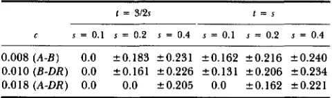
Level of disequilibrium D expected for given s and t values for the recombination amount between HLA loci A, B, and DR

t = 312s t = s

C s = 0.1 s = 0.2 s = 0.4 s = 0.1 s = 0.2 s = 0.4

0.008 (A-B) 0.0 20.183 20.231 20.162 20.216 20.240 0.010 (B-DR) 0.0 20.161 20.226 20.131 20.206 20.234 0.018 (A-DR) 0.0 0.0 20.205 0.0 20.162 k0.221

Now let us assume that c

>

0. In this case, we must iterate the expressions for the genotypic frequencies given above. Using the results from c = 0 as a background, we can organize the results, given that there is recombination, in a similar manner. When t

>

2s, then the only equilibrium present is

D

= 0. In addition, when t = 2 s ) the only equilibrium is for D = 0 , unlike the c = 0 case. If t

<

2 s , then there are

D # 0 equilibria if the recombination is low enough. Table 3 gives several such cases, including t = Y2s and t = s. The middle column gives the multiplicative case, i.e., if wAB = (1 - s)* = 1

-

t so

that t = 1

-

(1

-

s ) ~ . For example, in the case analogous to multiplicative fitness values and assum- ing s = 0.1 (making t = 0.19)) then if c

<

0.002

there are D # 0 equilibria. T h e least restrictive situation here is when s = t. For example, when t = s = 0.1, then if c

<

0.014, there are D # 0 equilibria.

How large is the disequilibrium generated by these selection and recombination values? Table 4 gives the

D

values for the map distances between the three

HLA loci A , B , and DR. Note that because

P I

= q 1

= Y2, and D = 1/40', where D ' is the normalized

disequilibrium measure of LEWONTIN (19641, and is the proportion of the maximum disequilibrium pos- sible. For example, when t =

Yzs,

s = 0.2, and c

Maternal-Fetal Interactions 211

TABLE 5

Frequency of mating types in which the male parent shares 0,

1, or 2 alleles with the female parent for HLA-A, or -B in a Danish sample (LARSEN and HANSEN 1987)

M Q MI M2

A 0.514 0.452 0.034

B 0.699 0.288 0.013

A o r B 0.384 0.422 0.172

DISCUSSION

A balancing selection model based on the immu- nological hypothesis developed to explain recurrent spontaneous abortion appears to have the potential to maintain a large amount of genetic polymorphism. As with incompatibility systems in plants, the ex- pected change in allelic frequencies and the equilib- rium allelic frequency decline as the number of alleles increases. As a result, genetic drift should become a stronger influence on allelic frequencies when there are more alleles (e.g., WRIGHT 1965). An excess of heterozygotes is predicted by this selection mode and occurs when there is strong selection. However, with weaker selection the genotypes are virtually in Hardy- Weinberg proportions.

There are three classes of mating types under this scheme, i.e., the male parent shares 0, 1, or 2 alleles with the female. As shown in Figure 3, the mating type with no shared alleles is most frequent when there are many alleles (with a relatively even distri- bution) in the population and the mating type with two shared alleles most common when there are few alleles. Table 5 gives the expected frequencies of the mating types based on the observed haplotypic fre- quencies for HLA-A and B with 12 and 20 alleles, respectively, in a Danish sample (LARSEN and HANSEN

1987). Notice that the proportion of matings that share no antigens is largest for both loci individually and that only a small proportion share two antigens. When both loci are considered simultaneously, 61.6% of the matings share one or more antigens (2.2% shared three or four antigens).

Because the

DR

locus has fewer alleles than A or

B , more matings should share alleles at

DR

than at

A and B . Higher antigen sharing could, therefore, possibly result in more selection from maternal-fetal interactions at

DR

than at A or B . In fact, it appears that the rate of recurrent spontaneous abortion is higher for DR than for A or B (THOMAS et al. 1985), consistent with this prediction.

In addition, this selection mode has the potential to generate gametic disequilibrium between alleles at HLA loci. Given that the effect of a second locus is less than that of the first, i.e., t

<

2s, then the known linkage between HLA loci can generate disequilib- rium. For example, when c = 0.008, the recombi-

nation level between A and B , and s = t = 0.1, 65% of the disequilibrium possible is generated.

The other model suggested as an explanation for the high rate of recurrent spontaneous abortion in couples that share HLA antigens is the genetic hy- pothesis (e.g., SCHACTER, WEITCAMP and JOHNSON 1984; HEDRICK 1988). This model assumes that there are recessive lethals in the HLA region that may become homozygous in the progeny of parents that share antigens. However, HEDRICK (1988) has sug- gested that this would seem to depend upon high disequilibrium between lethals and a number of HLA antigens. In addition, such a selection mode would not result in stable polymorphism or stable disequi- librium at the HLA loci.

There are a number of other modes of selection, including resistance to pathogens, segregation dis- tortion, and non-random mating that have been suggested to be important for major histocompati- bility complex loci [see HEDRICK, THOMSON and KLITZ

(1987) for a review]. However, along with the path- ogen resistance mode, selection involving maternal- fetal interaction shows the most promise towards explaining genetic variation in the HLA region.

This research was supported by National Institutes of Health grants GM 35326 and HD 12731. We thank B. KLITZ, E. LOVIS, H. PAYAMI, and W. ROBISSOX for comments on the manuscript.

LITERATURE CITED

ALBERT E., M. BAUR and W. MAYR, 1984 Histocompatibility Testing

1984. Springer-Verlag, Berlin.

CLARKE B., and D. R. S . KIRBY, 1966 Maintenance of histocom- patibility polymorphisms. Nature 211: 999-1000.

FELDMAN M. W., I. FRAXKLIN and G. THOMSON, 1974 Selection in complex genetic systems. I. The symmetric equilibria of the three-locus symmetric viability model. Genetics 76: 135-162. GILL T. J., 1983 Immunogenetics of spontaneous abortions in

humans. Transplantation 35: 1-6.

HEDRICK P. W., 1988. HLA-sharing, recurrent spontaneous abor- tion, and the genetic hypothesis. Genetics 119: 199-204. HEDRICK P. W., and G . THo\rsos, 1983 Evidence for balancing

selection at HLA. Genetics 104: 449-456.

HEDRICK P. W., and G. THOMSOX, 1986 A two locus neutrality test: Applications to humans, E . coli, and lodgepole pine. Genetics 112: 135-156.

HEDRICK P. W., G. THOMSOX and W. KLITZ, 1987 Evolutionary genetics and HLA: Another classic example. Biol. J. Linn.

HULL P., 1966 Possible stability of polymorphism in a multiallele incompatibility system in the mouse. Genetics 54: 1049-1053. KLITZ W., and G. THOMSON, 1987 Disequilibrium pattern anal- ysis. 11. Application to Danish HLA-A and -B data. Genetics

LARSEN S. D., and H. E. HANSEN, 1987 Antigen sharing in couples in a two-locus ABO-like system. Ann. Hum. Genet.

51: 177-180.

LEWOHTIX R. C., 1964 The interaction of selection and linkage. I. General considerations; heterotic models. Genetics 49: 48- 67.

MCLAREX A., 1975 Antigenic disparity: does it affect placental size, implantation or population genetics. In: Immunobiology of

Trophoblast. Clinical and Experimental Immunoproduction I , Edited SOC. 31: 311-331.

212 P. W. Hedrick and G . Thomson

by R. G . EDWARDS, C. W. S. HOWE and M. H. JOHNSON. T. J. GILL, 1985 HLA sharing and spontaneous abortion in

Cambridge University Press, Cambridge. humans. Am. J. Obstet. Gynecol. 151: 1053-1058.

SCHACTER B., L. R. WEITCAMP and W. E. JOHNSON, 1984 Parental WARBURTON F. L., 1968 Maintenance of histocompatibility PO-

HLA compatibility, fetal wastage, and neural tube defects: lymorphism. Heredity 23: 151-152.

evidence for a TIt-like locus in humans. Am. J. Hum. Genet. WRIGHT S . , 1965 The distribution of self-incompatibility alleles

THOMAS M. L., J. H. HARCER, D. K. WACENER, B. S . R A B I N and Communicating editor: W. J. EWENS