Statistical Methods for Optimal Dose Finding.

(1)

ABSTRACT

ZHU, LIANGYU. Statistical Methods for Optimal Dose Finding. (Under the direction of Wenbin Lu and Rui Song.)

Statistical methods are becoming increasingly popular for optimizing drug doses in clinical trials. In a typical dose-finding trial, a single optimal dose is decided at the end of the trial and is recommended to all future patients. However, patients might respond differently to the same dose of a drug due to differences in their physical conditions, genetic factors, environmental factors and medication history. Taking patient heterogeneity into consideration when making dose decisions is essential for achieving better treatment results. Traditionally, personalized treatment finding process requires repeating clinical visits of the patient and frequent adjustments of the dosage. Thus the patient is constantly exposed to the risk of underdosing and overdosing during the process. Data driven methods for finding optimal personalized dosage have the potential to shorten the process and lower the risk for the patient. Existing statistical methods for finding personalized treatments are mostly restricted to a finite number of treatment options. In this dissertation, we study the statistical methods for finding the optimal personalized treatment when the treatment options are continuous. The problem is studied under the single-stage setting and the mobile health setting.

In Chapter 2, we study the statistical methods for finding optimal personalized doses under the single-stage setting. We review the existing statistical methods for personalized treatment finding. A kernel-assisted learning method is then proposed for estimating the optimal personalized dosage. Theoretical results and simulation studies are provided for the proposed method. This method is then applied to a wafarin dataset.

(2)

(3)

(4)

Statistical Methods for Optimal Dose Finding

by Liangyu Zhu

A dissertation submitted to the Graduate Faculty of North Carolina State University

in partial fulfillment of the requirements for the Degree of

Doctor of Philosophy

Statistics

Raleigh, North Carolina 2020

APPROVED BY:

Marie Davidian Michael Kosorok

Wenbin Lu

Co-chair of Advisory Committee

Rui Song

(5)

DEDICATION

(6)

ACKNOWLEDGEMENTS

(7)

LIST OF TABLES

Table 2.1 Summary of simulation settings . . . 24

Table 2.2 Simulation results from 500 replicates for randomized trials and observational studies. . . 25

Table 2.3 Value estimate V(ˆπ) from 500 simulations in settings 1-4 . . . 26

Table 2.4 Average ˆβn from 500 replicates for setting 5 . . . 28

Table 2.5 Value estimate V(ˆπ) from 500 simulations in setting 5 . . . 28

Table 2.6 Estimated ˆβ with warfarin data with kernel assisted learning . . . 30

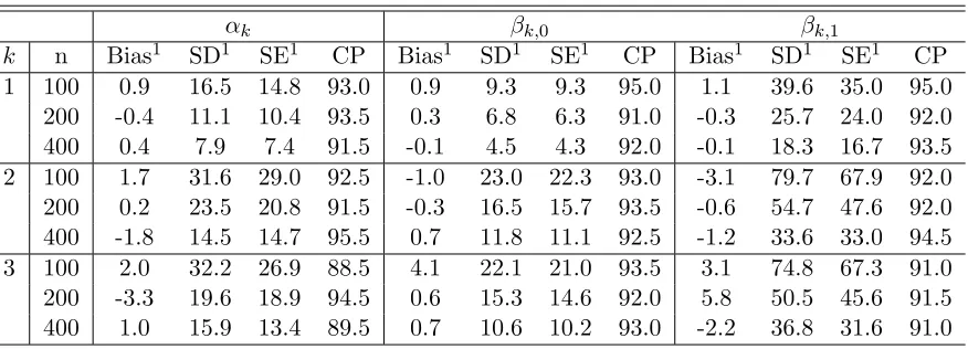
Table 3.1 Simulation results from 200 replicates for observational studies. . 64

Table 3.2 Estimated Parameters for Lag 3 Weighted Advantage from 200 Replicates . . . 65

Table 3.3 Simulation results from 200 replicates when θ2 =−0.1. . . 65

Table 3.4 Estimated Parameters for Lag 3 Weighted Advantage from 200 Replicates When θ2 =−0.1 . . . 65

Table 3.5 Estimated variables with the Ohio type 1 diabetes dataset . . . . 69

(10)

LIST OF FIGURES

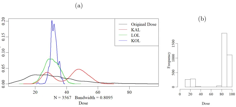
Figure 2.1 Distribution of the variables in the warfarin dataset. . . 31 Figure 2.2 Empirical distribution of suggested doses of several methods for

the walfarin dataset. In panel (a), the black line is the distribution of the original doses from the dataset. The green line denotes the result from linear O-learning. The blue line denotes the result from kernel based O-learning. The red line denotes the result from kernel assisted learning. Panel (b) is the histogram of the suggested doses using discretized Q-learning. . . 31 Figure 2.3 Empirical distribution of the estimated value function over 200

(11)

CHAPTER

1 INTRODUCTION

The goal of dose-finding is to come up with safe and efficient drug administration in humans given a certain medical condition. Typical dose-finding trials happen at early phases of clinical experiments where different doses of a new drug are evaluated. An ideal dose-finding study is conducted by a double-blind randomized trial where each patient is randomly assigned a dose among a few safe dose levels for a candidate drug (Chevret 2006). At the end of the trial, a single dose leading to the best average response is determined as a recommendation for future patients. Here, the response is defined as an outcome of interest, it can include measurements of the therapeutic effect of the treatment and the negative symptoms that appear under the clinical or the laboratory settings due to the toxicity of the treatment. Therefore, dose-finding is the art of maximizing the therapeutic effect of the drug while managing the toxicity of the drug at an acceptable level.

(12)

visits of the patient and frequent adjustments of the dosage. Thus the patient is constantly exposed to the risk of underdosing and overdosing during the process. Data driven methods for finding the optimal personalized dosage have the potential to tremendously shorten the process and lower the risk for the patient.

1.1 Motivation

Statistical methods are becoming increasingly popular for optimizing drug doses in clinical trials. However, existing methods for finding the optimal personalized treatments are mostly restricted to the scenario where there are a finite number of treatment options. In particular, people are interested in finding individualized treatment rules (ITR), which output a treatment option within a finite number of available treatments based on patient level information. Such treatment rules can thus be used to guide treatment decisions aiming to maximize the expected clinical outcome of interest, also known as the expected reward or value. An optimal treatment rule is defined to be the one that maximizes the value in the population among a class of treatment rules. Various statistical learning methods have been proposed to infer optimal individualized treatment rules using data from randomized trials or observational studies. Existing methods include model-based approaches, such as Q-learning (Watkins and Dayan 1992; Zhao et al. 2009; Qian and Murphy 2011; Schulte et al. 2014) and A-learning (Murphy 2003; Robins 2004; Henderson et al. 2010; Schulte et al. 2014), and direct value search methods by maximizing a nonparametric estimator of the value function (e.g. Zhang et al. 2012a,b; Zhao et al. 2012).

(13)

process, which lasts from weeks to months, the patient is constantly under the risk of overdosing or underdosing. Nowadays, there are organizations gathering an abundant amount of data associated with individual warfarin therapies, including the medical history, the demographic information, the genetic factors, and the therapeutic dosage of the patients. Data-driven methodologies for finding personalized dosages are made possible by the availability of these datasets. A data-driven dosage estimation method has the potential to greatly speed up the dosing process and exempt the patients from the risks of incorrect dosages. Therefore, in this dissertation, we study the statistical methods for providing personalized dosage suggestions which optimize the outcome of interest.

(14)

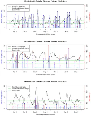
with simple mathematical operations using planned carbohydrate intake and measured blood glucose (Arnhold et al. 2014). However, the insulin dosage calculation varies largely among patients according to their personal insulin sensitivity factor and carbonhydrate factor (Huckvale et al. 2015). These simple dose rules fail to adapt to the variability among patients and might lead to incorrect dosage suggestions. In addition, the insulin absorption rate can be influenced by other factors including patients’ physical activity level and the temperature of the environment. An ambient temperature of 30 Celsius degrees can speed up the insulin absorption by two to four times compared to an ambient temperature of 10 Celsius degrees (Zisser et al. 2008). Therefore, an individualized dose recommendation system based on the time-varying physical condition of the patient is needed for an accurate estimation of the optimal personalized dosage. However, analyzing mobile health data can be challenging because there are typically a large number of time points, time-varying treatments, and a non-definite time horizon (Luckett et al. 2019). In this dissertaton, we also study the statistical methodologies for providing individualized dose suggestions using mobile health data. A detailed outline of the dissertation is given below.

1.2 Outline

The structure of the dissertation is as follows.

In Chapter 2, we focus on statistical methodologies for optimal dose finding. We first review the existing statistical methods for finding optimal individualized treatment rules. The limitations of these methods when applied to continuous dose suggestions are discussed. We then present existing methodologies for finding optimal individualized dose rules (IDR), which output dose suggestions within a safe dose range based the information of the patients. These methodologies are either limited by strict model assumptions for the expected outcome, or have provided no statistical inference for the estimated optimal dose rules. Therefore, we propose a kernel-assisted learning (KAL) method which requires no model assumption for the expected outcome and is capable of providing statistical inference for the estimated dose rules. Theoretical results and simulation studies are presented for the proposed method. It is then applied to a warfarin dataset collected by Consortium (2009).

(15)

the limitations of these methods when applied to mobile health data. Then we extend the definition of lagged treatment effects by Luckett et al. (2019) to continuous doses under the mobile health setting. A kernel-assisted learning method based on structural nested models (Robins 1994, 2004) is proposed for estimating this lagged treatment effect. Next, we focus on providing dose recommendations based on the estimated lagged treat-ment effects. Existing treattreat-ment recommendation strategies under infinite time horizons typically aim at maximizing an accumulated long-term reward. However, for diseases such as high blood pressure or hyperglycemia, the mobile health interventions actually aim at monitoring adverse events in a short term (Haller et al. 2004; Heron and Smyth 2010). Maximizing the cumulative reward might not be the optimal criteria for providing treatment suggestions under this scenario. Therefore, we define a weighted advantage for the doses as a measurement of the treatment effect over a short period of time. We then estimate the optimal dose which maximizes this weighted advantage. Theoretical results and simulation studies are presented for this estimation method. Finally, we apply the proposed method to the Ohio type 1 diabetes dataset and estimate the optimal dosage for the rapid-reacting insulin doses. Results are presented and discussed at the end of Chapter 3.

1.3 Notations

In this dissertation, we use capital letters such asA, X, Y to denote random variables and lowercase letters such as a, x, y to denote specific values taken by the random variables. The probability mass function of a discrete random variable X is written as pX(·). The

probability density function of a random variable X is written as fX(·). For any

one-variable functiong(·), the first, second and third order derivative of g(·) are written as ˙

g(·), ¨g(·), ...g_{(·). We use} _{I(·) to denote the indicator function. For example} _{I(X >} _{0) is} equal to 1 if X > 0 and is equal to 0 if X ≤ 0. For a matrix Σ, |Σ| is used to denote the determinant of the matrix. Under the mobile health setting where data are collected at multiple time points t = 1, . . . T. We use ¯Xt to denote the history of a variable X

up to time point t: ¯Xt ={X1, . . . , Xt}. Xt denotes the the random variable from time

t to T: X_t = {Xt, Xt+1, . . . , XT}. Let ¯X denotes the complete history of variable X:

¯

X = {X1, . . . , XT}. For any function g(·) of a random variable X, Png(X) is used to

denote the empirical average of the function: _Png(X) =Pn

(16)

CHAPTER

2 KERNEL ASSISTED LEARNING FOR

SINGLE-STAGE PERSONALIZED DOSE

FINDING

2.1 Introduction

(17)

(Zhang et al. 2012a,b; Zhao et al. 2012).

The above methods, however, are not directly applicable when the number of possible treatment levels is large. Using continuous individualized dose rules (IDR), where a dose level is suggested within a safe dose range, can better adapt to patient heterogeneity in drug response. Extending the above methods for finding optimal individualized treatment rules to continuous treatment options is non-trivial. Several methods have been proposed for finding optimal individualized dose rules. One way of extending existing methods to the continuous dose case is to discretize the dose levels. Laber and Zhao (2015) proposed a tree-based method and turned the problem into a classification problem by dividing patients into subgroups and assigning a single dose to each subgroup. Chen et al. (2018) extended the outcome weighted learning method (Zhao et al. 2012) from binary treatment settings to ordinal treatment settings. However, in cases where patient responses are sensitive to dose changes, a discretized dose rule with a small number of levels will fail to provide dose recommendations leading to optimal clinical results. On the other hand, a discretized dose rule with a large number of levels may result in limited observations within each subgroup, and thus may be at risk of overfitting.

Alternatively, Rich et al. (2014) extended the Q-learning method by modeling the interactions between the dose level and covariates with both linear and quadratic terms in doses. However, such a parametric approach is sensitive to model misspecification and the estimated individualized dose rule might be far away from the true optimal dose rule. In addition, it cannot be guaranteed that the estimated optimal dose falls into the safe dose range. More recently, Chen et al. (2016) extended the outcome weighted learning method proposed by Zhao et al. (2012) and transformed the dose-finding problem into a weighted regression with individual rewards as weights. The optimal dose rule is then obtained by optimizing a non-convex loss function. This method is robust to model misspecification and has appealing computational properties, however, the associated statistical inference for the estimated dose rule is challenging to determine.

(18)

derived based on nontrivial calculations of the expectation of a U-statistic.

The remainder of the chapter is organized as follows. In Section 2.2, we present the problem setting and the notations for optimal dose finding. In Section 2.3, existing methods for finding the optimal ITR and the optimal IDR are reviewed. Our proposed method is presented in Section 2.4. The theoretical results of the estimated parameters are established in Section 2.5. In Section 2.6, we demonstrate the empirical performance of the proposed method via simulations. In Section 2.7, the proposed method is further illustrated with an application to a warfarin study. Some discussions and conclusions are given in Section 2.8. Proofs of the theoretical results are provided in Section 2.9.

2.2 Problem Setting

We first present the single-stage personalized dose-finding problem with a statistical framework. Assume that the observed data consist of n independent and identically distributed observations {(Xi, Ai, Yi)}ni=1, where Xi ∈ X is a q-dimensional vector of

covariates for the ith patient, Ai ∈ Ais the dose assigned to the patient with A being

the safe dose range (if A is a set of finite number of treatment options, then the problem transform into finding the optimal individualized treatment rule), and Yi ∈ R is the

observed outcome of interest after the treatment Ai is given to the patient. Without

loss of generality, we assume that larger Y means better outcome. Letπ(X) denote an individualized dose rule, which is a deterministic mapping function fromX to A. To define the value function of an individualized dose rule, we use the potential outcome framework (Rubin 1978). Specifically, let Y∗(a) be the potential outcome that would be observed when a dose level a ∈ A is given. Define the value function as the expected potential outcome in the population if everyone follows the dose rule π, i.e. V(π) =E[Y∗{π(X)}]. The optimal individualized dose rule is defined as πopt = arg maxπ∈GV(π), where G is a

class of interested dose rules. For example, a linear class of dose rules can be written as: G ={πβ(X) =βTX :β ∈Rq}.

In order to estimate the value function from the observed data, we need to make the following three assumptions similar to those adopted in the causal inference literature (Robins 2004).

• Y =R

Aδ(A =a)Y

∗_{(a)da, where} _{δ(·) is the Dirac delta function. This corresponds}

(19)

This assumption implies that there is no interference among patients. In the case where the treatment options are discrete, this assumption can be written as: Y =

P

a∈AI(A=a)Y ∗_(a).

• The potential outcomes{Y∗_{(a) :} _a_{∈ A}}_{are conditionally independent of}_A_given_X,

which is also known as the no unmeasured confounders assumption. This assumption can be naturally satisfied by the design of a randomized dose trial. However, it cannot be validated in an observational study.

• There exists a c >0 such that fA|X(A =a|X =x)≥cfor all a∈ A, x∈ X, where

fA|X(a|x) is the conditional density ofA= agiven X =x. In the discrete treatment

case, the assumption can be written as:pA|X(A=a|X =x)>0 for alla∈ A, x∈ X.

This assumption ensures thatV(π) can be estimated using the observed data for all π:X → A. This is also known as the positivity assumption.

Under these assumptions, we can show that V(π) can be estimated with the observed data :

V(π) = E[Y∗(π(X))]

=EX[E{Y∗(π(X))|X}]

=EX[E{Y∗(π(X))|A=π(X), X}]

=EX[E{Y|A=π(X), X}].

The second equation above is based on the basic property of conditional densities. The third equation above is valid because of the no unmeasured confounder assumption. The fourth equation is based on the consistency assumption. The positivity assumption ensures that the right side of the last equation can be estimated empirically.

2.3 Literature Review

2.3.1 Methods for Finding Discrete Optimal Treatment Rules

Regression Based Method

(20)

this model is correctly specified, then there exists some ˜β where µ(A, X) =µ(A, X; ˜β). The optimal treatment rule would be πopt_{(X) = arg max}

πµ(π(X), X) =I{µ(1, X; ˜β)>

µ(0, X; ˜β))}. Therefore, we can estimate the optimal dose rule by obtaining an estimate of the parameters from the data, ˆβ. Then ˆπopt_{(X) =} _I_{{µ(1, X}_{; ˆ}_β) _{> µ(0, X; ˆ}_{β)}. The}

estimation of the parameters can be achieved through standard ordinary least squares (OLS) or weighted least squares (WLS). An estimate of the maximum value function

V(πopt) = E{Y∗_(πopt_)} _{would be:}

1 n

n

X

i=1

h

µ(1, Xi,β)ˆˆ πopt(Xi) +µ(0, Xi,β){1ˆ −πˆopt(Xi)}

i

.

Extension of this method to more than two treatments is straightforward. However, an obvious drawback of this method is that the estimated treatment rule may be far away from the optimal rule when the posited model is not correct. The estimated maximum value function might not converge to the true maximum value function in such cases.

Notice that the optimal treatment rule in this case πopt(X) = I{µ(1, X)> µ(0, X))} only depends on the contrast, which is the difference of the expected reward between the treatments given the patient’s information, C(X) =µ(1, X)−µ(0, X). The A-learning method (Blatt et al. 2004; Robins 2004; Moodie et al. 2009; Henderson et al. 2010; Wallace and Moodie 2015) utilizes this idea by positing a model for the contrast function, say C(X;ψ). The original µ-function can be written asµ(A, X) =h(X) +A×C(X;ψ), where the form of h(X) =µ(0, X) does not need to be specified. The optimal treatment rule would thus be πopt ₌_I{C(X)_>_{0}). Let ˜}_{p(X) =}_p(A_{= 1|X) be the propensity score of}

receiving treatment A= 1. Robins (2004) shows that the parameters ψ can be estimated consistently by the following estimation equation:

n

X

i=1 λ(Xi)

n

Ai−p(X˜ i)

o

×nYi−AiC(Xi;ψ)−θ(Xi)

o

= 0. (2.1)

where λ(Xi) is an arbitrary function with the same dimension as ψ and an arbitrary

function θ(X). This method is also referred to as g-estimation. Robins (2004) also shows that, if the model C(X;ψ) is correct and var(Y|X) is constant, the optimal choice of λ(X;ψ) will be ∂C(A, X;ψ)/∂ψ, and the optimal choice of θ(X) will beh(X).

(21)

a consistent estimator of ψ as long as one of these two models is correctly specified. After the estimated parameter ˆψ is obtained, the estimated optimal dose rule would be

ˆ

πopt_{(X) =} _{I{C(X; ˆ}_ψ)_>_0}.

Compared to the Q-learning method, the A-learning method is more robust to model misspecification because the exact form of the expected reward function does not need to be specified. Extensions to more than two-treatments (see Robins 2004; Moodie et al. 2007) are possible with more complicated formulations. However, the performance of the method still largely depends on the correct specification of the model for the contrast functionC(X). Schulte et al. (2014) also show that when the models for Q-learning and A-learning are both correctly specified, the A-learning might yield relatively inefficient inference forψ without an optimal choice of λ. Furthermore, extensions to the continuous dose finding problem are not feasible because the contrast function cannot be easily defined with an infinite number of treatment options.

Inverse Probability Weighted Estimation Method

In certain cases, the treatment rule can be defined by a simplified class of rules involving only a subset of the covariates (Zhang et al. 2012b). For example, if µ(A, X;β) = β1X1+A(β2X2+β3X3), then the optimal treatment rule would beI{X2+ (β3/β2)X3 >0} or I{X2+ (β3/β2)X3 <0]} depending on the sign of β2. Therefore, the optimal treatment can be defined by the parameter space {η:η =β2/β3}. Let the class of treatment rules of the form πη(X) = π(X, η) = I(X2 +ηX3 > 0) or I(X2 +ηX3 < 0) be Gη. Zhang

et al. (2012b) proposed a more robust method by directly searching for the optimal treatment rule within the class Gη without assuming any models forµ(A, X). The goal

thus becomes to find ηopt = arg maxηE{Y∗(πη)}. This can be achieved by first obtaining

a nonparametric approximation of E{Y∗_(π

η)}, then find the ˆη which maximizes the

approximated value function.

However, for a specific treatment ruleπη, the potential outcomeY∗(πη(x)) is probably

not observed for somex∈ X. Thus, estimating the value function can be regarded as a miss-ing data problem, where {Y∗_(π

η)(X), X} is the full dataset and {I(A =πη(X)), Y I(A =

πη(X)), X} is the observed dataset. Zhang et al. (2012b) proposed to estimate the value

function with an inverse probability weighted estimator (IPWE). Assume that the data come from a randomized trial where the propensity score ˜p(X) =p(A= 1|X) is known. (In observational studies where the propensity score is unknown, it can be estimated by a

parametric model, say ˜p(X;γ).) Let ˜pc(X;η) = ˜p(X)π(X, η) +{1−p(X)}{1˜ −π(X, η)}

(22)

η, the inverse probability weighted estimator of the value function is:

IPWE(η) = 1 n

n

X

i=1

YiI{Ai =πη(X)}

˜

pc(Xi;η)

= 1 n

n

X

i=1

YiI{Ai =πη(X)}

˜

p(Xi)Ai{1−p(X˜ i)}1−Ai

. (2.2)

This estimator is shown to be consistent for E{Y∗_(π

η)} when ˜p(X) is known or ˜p(X;γ)

is a correctly specified model for ˜p(X) (Cao et al. 2009) . Cao et al. (2009) also proposed another estimator of the value function with improved robustness. It is known as the augmented inverse probability weighted estimator (AIPWE):

AIPWE(η) = 1 n

n

X

i=1

nY_iI{A_i =π_η(X_i)}

˜

pc(Xi;η)

−I{Ai =πη(Xi)} −p˜c(Xi;η) ˜

pc(Xi;η)

m(Xi;η,β)ˆ

o

,

(2.3) where,

m(X;η, β) = µ(1, X;β)π(X, η) +µ(0, X;β)n1−π(X, η)o is an approximation for E{Y∗_(π

η)}; µ(A, X;β) is a working model for E(Y|A, X) with

parameters β; ˆβ can be obtained using regular regression methods. The AIPWE is consistent forE{Y∗_(π

η)}as long as ˜p(X) is known, or a correct model is specified for ˜p(X),

orµ(A, X;β) is correctly specified. If the propensity score is known or can be approximated with a correctly specified model, the estimation efficiency is improved when the working model µ(A, X;β) is also correctly specified (Zhang et al. 2012b). Then the estimated optimal treatment rule is ˆπopt_η = π(X,ηˆopt), where ˆηopt maximizes the corresponding estimator of the value function: ˆηopt= arg maxηIPWE(η) or ˆηopt = arg maxηAIPWE(η).

(23)

Outcome Weighted Learning

Another direct method is the outcome weighted learning (O-learning) method proposed by Zhao et al. (2012). The optimal treatment rule is regarded as a classification problem where the goal is to classify the patients into groups by their optimal treatments. Instead of maximizing an approximate of the value function, the outcome weighted learning method finds the optimal rule by directly minimizing a loss function which can be interpreted as a classification error. Assume that the data is from a randomized trial where ˜p(X) =p(A= 1|X) is a constant ˜p, and assume that there are only two treatment options A={0,1}. The value function can thus be written as:

V(π) =E{Y∗(π)}=EnY I(A=π(X)) p(A|X)

o

=En Y I(A=π(X)) ˜

pA+ (1−p)(1˜ −A)

o

. (2.4)

Maximizing Equation (2.4) is equivalent to minimizing:

E(Y|A= 1) +E(Y|A=−1)−V(π) =En Y I(A6=π(X)) ˜

pA+ (1−p)(1˜ −A)

o

. (2.5)

If we regard π(X) as a classification of the patients into two groups corresponding to the two treatment and weigh each misclassification event by Y /{˜pA+ (1−p)(1˜ −A)}, the right side of Equation (2.5) will be an expectation of the classification error and can thus be estimated by the empirical classification error:

1 n

n

X

i=1

Yi

˜

pAi+ (1−p)(1˜ −Ai)

I{Ai 6=π(Xi)}.

Notice that with this method, we would prefer a classification which is consistent with the assigned dose where the observed outcome is large. When the observed outcome is small, the assigned treatment is less likely to be recommended by the treatment rule. Similar to the robust method proposed by Zhang et al. (2012b), we search for the optimal treatment rule within the class of treatment rules Gη in the form of πη(X) =π(X;η) =I{g(X;η)>0},

where g(X;η) is a prespecified function of X indexed by parameterη. The optimization problem thus becomes:

ˆ

ηopt = arg min

η

1 n

n

X

i=1

Yi

˜

pAi+ (1−p)(1˜ −Ai)

InAi 6=I(g(Xi;η)>0)

o

. (2.6)

(24)

this issue by substituting the indicator functionI{g(X;η)>0}with a hinge loss function {1−Ag(X;η)}+ _where _x+_{= max(x,}_{0) (see Cortes and Vapnik 1995). A penalty term is} added for the complexity of the treatment rule to avoid overfitting. Then,

ˆ

ηopt = arg min

η

1 n

n

X

i=1

Yi

˜

pAi+ (1−p)(1˜ −Ai)

{1−Aig(Xi;η)}++λnkπηk2, (2.7)

where kπk is some seminorm for π (For example, whenπη(X) = I{XTη >0}, then kπηk

can be the Euclidean norm ofη), and λnis a tuning parameter which controls the strength

of the penalty on the complexity of the treatment rule.

Both Zhang et al. (2012b)’s method and Zhao et al. (2012)’s method are based on finding an optimal treatment rule within a class of rules by optimizing an objective function. Zhang et al. (2012a) further extended these methods by providing a framework which unifies both of these methods into a weighted classification problem where the class of treatment rules does not need to be prespecified. However, this classification perspective is not feasible when the treatment options are continuous. Extensions of these methods to continuous dose finding are nontrivial.

2.3.2 Methods for Finding Optimal Dose Rules

The methods discussed in Section 2.3.1 provide different approaches to the problem of optimal treatment finding. However, when the number of possible treatment levels is large, the application of these methods would be problematic. For example, the dosage for the drug warfarin (as mentioned in Chapter 1) typically range from 10 mg to 100 mg weekly. Classifying the doses into 91 different levels and regarding this as a discrete treatment finding problem would not be ideal because each level would be only assigned to a small number of patients. Estimation of the value function might thus have large variance. The information in the data would not be used efficiently either. Regarding the treatment options as continuous doses is more appropriate in such cases. A randomized dose trial, where each patient is randomly assigned a dose within a safe dose range, is needed for finding optimal treatment rule with continuous doses. Such rules are also known as individualized dose rules (IDR). In the following discussion, we assume that A is an interval of the safe dose range. Without loss of generality, we assume thatA = [0,1].

Discretized Dose Rules

(25)

extended the AIPWE method of Zhang et al. (2012b) by first discretizing the treatment levels into a finite number of treatments, and then transforming the optimal treatment rule finding problem into a clustering problem among the patients. Similar to the method proposed by Zhang et al. (2012b), Laber and Zhao (2015) proposed to directly search for the optimal rule within a class of treatment rules, which is the class of treatment rules that can be represented by decision trees in this case. The optimal rule is estimated by maximizing an approximation of the value function. Within the context of a clustering problem, the objective function to maximize (the approximated value function) can be regarded as the purity measure for evaluation of the quality of the clustering (see Larson 2010). The optimal treatment rule within the class can thus be found by establishing a decision tree, where the algorithm recursively partition the covariate space into rectangular sets based on maximizing the total purity measure (see Breiman 1984; Hastie et al. 2009, for details).

Methods like IPWE and AIPWE are not directly applicable for estimating the value function, because the assigned doses to each patient are not restricted to the discretized dose levels. The probability of observing the outcome of the dose levels suggested by the corresponding rule would be 0. Laber and Zhao (2015) proposes a smoothed version of the AIPWE by replacing the indicator function I{a = π(x)} in Equation (2.3) with a kernel smoother: vπ,h(a|x) = h−1k

g(a)−g(π(x))}/hg(a), where˙ k(·) is a symmetric density function, h is the bandwidth, g(·) is a prespecified one-to-one function from the treatment space to_R and ˙g(·) is the derivative of the function g(·). One simple example of the kernel smoother would be vπ,h(a|x) = (2h)−1g(a)I˙

n

|g(a)−g(π(x))| ≤ ho. The treatment ruleπ(x) can thus be approximated by a class of distributions over A that has the mass around π(x). A smoothed version of the value function V(π) =E{Y∗_(π)} _can

be written as EnY vπ,h(A|X)/fA|X(A|X)

o

. Here, the fA|X(a|x) is the conditional density

of A given X. A smoothed version of the AIPWE estimator in Equation (2.3) would be: 1

n

X

i=1

hY_i−m(X_i;β) v_π,h(A_i|X_i)

fA|X(Ai|Xi)

+m(Xi;β)

i

, (2.8)

wherem(X;β) is a parametric model forµ(A, X) with parametersβ. Maximizing Equation (2.8) is equivalent to maximizing:

ˆ

C(π) =n−1h{Yi−m(Xi;β)}vπ,h(Ai|Xi) fA|X(Ai|Xi)

i

.

(26)

that for a subset of the covariate space r ⊂ X, πr,a,a0 denotes the rule that assigns

treatment a for all x ∈ r and treatment a0 for all x ∈ rc_{, where} _{a, a}0 _{are within the}

discretized treatment space. For a node defined with a subset of the covariate space ˜r ⊂ X and another subset r⊂ X, the purity measure of partitioning ˜r into ˜r∩r and ˜r∪rc _is

defined as: P(˜r, r) =

"

Pn

Y −m(X,β)ˆ I(X ∈r)v˜ πr,a,a0,h

A|X fA|X(πr,a,a0(X)|X)

#"

Pn

I(X ∈r)v˜ πr,a,a0,h

A|X fA|X(πr,a,a0(X)|X)

#−1

. (2.9)

The algorithm starts from the root node defined by the whole parameter space. Each time it finds the split of a node where the purity measure is maximized. The algorithm ends when the maximal increase of purity measure is below a predefined threshold. The rule that corresponds to the partition of the final tree is the estimated optimal treatment rule.

This tree-based method provides an approach to extension of an existing method to finding optimal dose rules. However, when the number of discretized intervals is small, the suggested dose rule may fail to provide a precise estimation of the optimal dosage for the patients. As the number of discretized intervals increase, the variance of the purity measure as defined in Equation (2.9) will increase tremendously because there are a limited number of observations within each interval. Therefore, continuous dose rules would better adapt to the complicated mechanisms of the drugs and the heterogeneous needs of the patients.

Regression based method

Another natural approach is to establish regression models for µ(A, X) = E(Y|A, X) just as when the treatment options are discrete. When the dose level is continuous, it is essential to consider a nonlinear relationship between the dose and the outcome, because overdosing often leads to toxicity while underdosing might result in inefficiency of the medicine. Rich et al. (2014) applied this idea and used a linear regression model including both quadratic terms and interaction terms between the covariates and the treatment. A general form of the model can be written as follows (Laber and Zhao 2015):

µ(A, X;ρ, θ, γ) = XTρ+XTθ(A−XTγ)2. (2.10) where ρ, θ, γ are the parameters to be estimated. If XT_θ _{is positive, the optimal dose rule}

(27)

interpreted as the effect of the covariates on the optimal IDR. It can be further extended to LASSO regression by including penalties of L2 norms of the parameters in the loss function while estimating the parameters (Chen et al. 2016). Other variations of the regression based method include support vector regression (SVR; Vapnik 2013; Smola and Sch¨olkopf 2004) and regression trees (Breiman 1984).

The estimated optimal dose rule by this method depends on the correctness of the model specified for µ(A, X). When the model is misspecified, the suggested dose rule may be far away from the true optimal dose rule. If XTθ is not always positive, then the suggested optimal dose rule will fall on the edges of the dose range, meaning that the suggested dose is either the maximum feasible dose or no dose at all, which is not ideal in practice. Even if XT_θ_ˆ_{is positive, the optimal dose estimated by} _XT_ˆ_γ _{may not fall into}

the safe dose range and thus not applicable in practice.

Outcome Weighted Learning

To avoid model misspecification, Chen et al. (2016) proposed a direct method by extending the outcome weighted learning method proposed by Zhao et al. (2012). Direct application of O-learning method to the continuous dose finding problem is not feasible because the probability of a certain dose a given covariates x ∈ X, denoted as pA|X(a|x) in

Equation (2.4), would be 0. Few subjects would satisfy Ai =π(Xi), which will make the

approximation of the value function unstable.

Chen et al. (2016) first extend Equation (2.4) by the replacing theIA= π(X) with an indicator function IA ∈ π(X)−φ, π(X) +φ , where φ is a bandwidth. They show that the ˜Vφ(π) defined below converges to the value function V(π) when φ converge to 0:

˜ Vφ(π) =

1 2φE

hY IA∈ π(X)−φ, π(X) +φ

fA|X(A|X)

i

, (2.11)

where fA|X here denotes the conditional density ofAgiven X. As a result, the πopt, which

maximizes ˜Vφ(π) and equivalently minimizes

EhY I

|A−π(X)|> φ 2φfA|X(A|X)

i

,

(28)

approximate the indicator function:

lφ

A−π(X)= min|A−π(X)|

φ ,1

. (2.12)

The function lφ can be written as the difference of two convex functions and thus the

difference of convex functions (DC) algorithm (see Le Thi Hoai and Tao 1997) can be used for the optimization of the loss function. The function to be minimized thus becomes:

Rφ(π) = E

hY l_φ A−π(X)

φfA|X(A|X)

i

, (2.13)

which can be estimated consistently with the empirical expectation: ˆ

Rφ(π) =Pn

Y lφn[A−π(X)] φnfA|X(A|X)

, (2.14)

where φn is some constant that goes to 0 as n goes to infinity. By including a term for

penalizing the complexity of π(X), the optimization problem is formalized as follows:

πopt = arg min

π

n

PnY lφn[A−π(X)]

φnfA|X(A|X)

+λnkπk2

o

, (2.15)

where λn is the tuning parameter which controls the complexity of the dose rule to avoid

overfitting.

The optimal dose rule which minimizes the loss function is searched directly within a class of rules. The author considers two classes of dose rules. The first class is the linear rules which can be written as π(X) = XTw+b. This method is also known as the linear outcome weighted learning (L-O-Learning). The second class is the non-linear rules defined in a reproducing kernel Hilbert space (RKHS) (see Vapnik 2013; Smola and Sch¨olkopf 2004). An RKHS HK associated with a symmetric continuous kernel function

K(·,·) : X × X →_R is the complete span of all functions K(·, X), X ∈ X. Then there exists a function Φ(·) that Φ(Xi)TΦ(Xj) = K(Xi, Xj). The dose rules from HK can

thus be represented by π(X) = wT_{Φ(X) +}_b _{(Vapnik 2013). The non-linear outcome}

weighted learning is therefore also known as kernel-based outcome weighted learning (K-O-Learning).

(29)

(30)

2.4 Kernel Assisted Learning

2.4.1 Method

In order to estimate the optimal IDR, we first estimateV(π) with a kernel based estimator and then estimate πopt _{by directly maximizing the estimated value function ˆ}_V_{(π). We}

search for the optimal individualized dose rule within a class of dose rules of the form: πβ(x) = π(x;β) ∈ G, where G = {g(βTx), β ∈ Rq}, and g : R → A is a predefined

link function to ensure that the suggested dosage is within the safe dose range. Let β∗ = arg maxβV(πβ), then the optimal IDR within G is:

π_βopt(X) =π(X;β∗) = arg max

π∈G V(π).

If the true optimal IDR: πopt _{= arg max}

πV(π) ∈ G, then π_βopt(X) = πopt. To see this,

we illustrate with a toy example. If the true model for E(Y|A, X) takes the form: E(Y|A, X) = ˜µ(X) + Q{A− g( ˜βT_{X)}H(X), where ˜}_{µ(X) is an unspecified baseline}

function, H(X) is a non-negative function and Q(·) is a unimodal function which is maximized at 0, then E(Y | A, X) is maximized at dose level A =g( ˜βT_{x) for patients}

with covariates X =x. Thus, the true optimal individualized dose rule is: πopt(X) = arg max

π V(π)

= arg max

π EX

h

EY |A=π(X), X i = arg max

π EX

h

˜

µ(X) +Q

π(X)−g( ˜βTX) H(X)i = arg max

π EX

h

Q

π(X)−g( ˜βTX) H(X)i =g( ˜βTX)∈ G.

The last equation above is true becauseQ{π(X)−g( ˜βT_{X)}H(X) is maximized at}_{g( ˜}_βT_X)

for each X ∈ X. If a unique maximizer of V(πβ) exists, then

β∗ = arg max

β V(πβ) = arg maxβ EX

h

Qg(βTX)−g( ˜βTX) H(X)i = ˜β.

Therefore, π_βopt = g(β∗TX) = πopt_{. Notice that if} _πopt _{= arg max}

πV(π) ∈ G/ , then

π_βopt 6=πopt_{. However,} _πopt

β is still of interest as long as the form of G is flexible enough,

because it maximizes the value function among this set of treatment rules. Therefore, we estimate β∗ using ˆβ = arg max ˆV(πβ), and the optimal IDR within G can be estimated

(31)

the conditional expectation E(Y|A, X) to apply this method.

Next, we propose a kernel based estimator for the value function. Let

M(β) =V πβ

=

Z

x∈X

mx, g(βTx)fX(x)dx,

where m(x, a) = E(Y | X = x, A = a) and fX(x) is the marginal density of X. Thus,

β∗ = arg maxβM(β). The functionm

x, g(βT_x)_{is estimated using the Nadaraya-Watson}

method given:

ˆ

mx, g(βTx)= 1

n

Pn i=1Yi_h1q

xKq(

x−Xi

hx ) 1

haK

g(βT_x₎₋_A i ha 1 n Pn i=1 1

hqxKq(

x−Xi

hx ) 1

haK

g(βT_x₎₋_A i

ha

, (2.16)

whereK(·) is a univariate kernel function andKq(·) is aqdimensional kernel function. Here,

hx andha are bandwidths that go to 0 as n→ ∞. Note that for simplicity of notification,

we use the same bandwidth for all dimensions of X here. In practice, we can use different bandwidths for different dimensions of X to increase the efficiency of the estimation. Moreover, the marginal density of X is estimated by ˆfX(x) = (1/n)Pn_i₌₁Kq{(x −

Xi)/hx}/hqx. The estimated value function can thus be written as:

Mn(β) =

Z

x

1

n

Pn

i=1Yi 1

hqxKq(

x−Xi

hx ) 1

haK

g(βT_X₎₋_A i ha 1 n Pn i=1 1

hqxKq(

x−Xi

hx ) 1

haK

g(βT_X₎₋_A i ha n1 n n X i=1 1 hqx

Kq(

x−Xi

hx

)

o

dx.

Then β∗ is estimated with ˆβn = arg maxβ∈ΘMn β

, where Θ is a compact subset of _Rq containingβ∗.

2.4.2 Computational Details

To implement the proposed method, the R package optimr() is used for optimization of the objective function (2.16). The integral inMn(β) is estimated by taking the average of

Ng random grid points in the covariate space. In our implementation, we choseNg = 3000.

In order to find the global maximizer of Mn(β), we start optimization from q different

initial points {(1,0, ...,0)T_,_(0,_1,_{0, ...,}₀₎T_{, ...,}_{(0, ...,}_0,₁₎T_} _{and choose the one that leads}

to the maximum objective function value. Denote the maximizer as ˆβn. When there is

only one continuous covariate included, following the theoretical rate of the bandwidth parameters, the bandwidths are chosen as hx = Cxsd(X)n−1/4.5, ha = Casd(A)n−1/4.5,

where Cx and Ca are constants arbitrarily taken between 0.5 and 3.5. When there are

(32)

Choosing the constants in the bandwidths is thus nontrivial. For the simulation setting 5, we arbitrarily choose the rate of the bandwidths as n−1/8 _{and then use 5-fold cross} validation to choose the constantsCx,Ca which minimize the mean squared error.

When the covariates consist of both continuous variables and categorical variables, the categorical variables are stratified for estimation of the value function. In other words, the kernel estimation is conducted within each subgroups classified by the categorical variables. Specifically, assume that X = (X₁T, X₂T)T ∈ X, where X1 is a q1 dimensional vector of continuous variables and X2 ∈ D is a q2 dimensional vector of categorical variables. The form ofMn(β) then becomes:

Mn(β) =

X

x2∈D

Z

x1

1

n

Pn

i=1YiK(x, X˜ i)_h1_aK

g(βT_X₎₋_A i

ha 1

n

Pn

i=1K˜(x, Xi) 1

haK

g(βT_X₎₋_A i ha 1 n n X i=1 ˜

K(x, Xi) dx1,

where x = (xT

1, xT2)T, Xi = (XiT1, XiT2)T, ˜K(x, Xi) = (1/hqx1)Kq1{(x1 −Xi1)/hx}I(Xi2 =

x2).

2.5 Theoretical Results

In this section, we establish the asymptotic properties of ˆβn. To prove these results, we

need to make the following assumptions. In the following expressions, ˙f(x), ¨f(x) and ...

f(x) denote the first, second and third derivatives of the functionf with respect tox; κ0,2 =

R

RK

2_(v)dv _{and ˙}_κ 0,2 =

R

˙

K2_(v)dv.

Assumption 2.1. 1 Assume that V is the set ofv ∈_R where K(v)˙ , K¨(v) andK...(v) exist. For h→0+ _as _n _{→ ∞} _{and constants} _l_,_u _{such that} _{l <}₀_{< u}_, R

[l/h,u/h]∩VK(v)dv = 1−

O(h2_), R

[l/h,u/h]∩VvK(v)dv = O(h),

R

[l/h,u/h]∩VK(v)dv˙ = O(h

3_), R

[l/h,u/h]∩V−vK(v)dv˙ =

1−O(h2_), R

[l/h,u/h]∩VK

2_(v)dv₌_κ

0,2 −O(h2),

R

[l/h,u/h]∩VK˙

2_(v)dv_{= ˙}_κ

0,2−O(h2),

R

[l/h,u/h]∩VK(v)dv¨ = O(h

4_), R

[l/h,u/h]∩VvK¨(v)dv = O(h

3_), R

[l/h,u/h]∩Vv

2_K(v)dv_¨ _{= 2}₋ O(h2), R_[_l/h,u/h_]_∩VK...(v)dv =O(h3), R_[_l/h,u/h_]_∩VvK(v)dv... = O(h2), R_[_l/h,u/h_]_∩Vv2K(v)dv... = O(h), R_[_l/h,u/h_]_∩Vv3K(v)dv... =O(1).

Assumption 2.2. The function M(β) = V(πβ) has a unique maximizer β∗.

Assumption 2.3. The function m(x, a) is uniformly bounded. The joint density function of X and A, fX,A(x, a), is uniformly bounded away from 0. In addition, the first, second, third and fourth order derivatives of m(X, A) and fX,A(X, A) with respect to X and A exist and are uniformly bounded almost everywhere.

(33)

Assumption 2.5. The derivatives for function g(·): g(β˙ T_X),_g(β_¨ T_X),..._g_(βT_X) _{exist and} are bounded almost everywhere.

Assumption 2.1 are regularity assumptions to ensure that the kernel estimators are unbiased. It is trivial to prove that it can be satisfied by most commonly used kernel functions such as the Gaussian kernel function, polynomial kernel, splines and all sufficiently smooth bounded kernel functions. Assumption 2.2 is an identifiability condition for β∗. Assumptions 2.3–2.5 ensure the existence of the limit of the expectation of Mn(β) and the existence of the covariance of the limiting distribution. In the following

two theorems, we establish the consistency and asymptotic normality of ˆβn, respectively. Theorem 2.1. Under assumptions 2.1–2.3, for hx,ha satisfying nhx2qh2a → ∞as n→ ∞, we have sup_β_∈_Θ|Mn(β)−M(β)| converge in probability to 0, whereΘ is a compact region containing β∗. Thus, βˆn= arg maxβ∈ΘMn(β) converge in probability to β∗.

Theorem 2.2. Under assumptions 2.1–2.5, for hx, ha satisfying nh2xqh2a → ∞ and

nhq

xh3a→ ∞ as n→ ∞, we have

(nhq_xh3_a)1/2( ˆβn−β∗)→N

n

0, D(β∗)−1ΣS(β∗)D−1(β∗)

o

in distribution as n→ ∞, where

D(β∗) =

Z

x

h

maa

x, g(βTx) g˙2(βTx) +ma

x, g(βTx) ¨g(βTx)ifX(x)xxTdx,

ΣS(β∗) =

Z

x

˙

g2(βTx)xxTκ0,2κ˙0,2fX2(x)

m2

x, g(xT_β) ₋_m2

x, g(xT_β)

fX,A

x, g(xT_β) dx,

and ma(x, a) =∂m(x, a)/∂a, maa(x, a) =∂2m(x, a)/∂a2, m2(x, a) =E(Y2 |X=x, A= a). Here, κ0,2 =

R

RqK

2

q(v)dv, κ˙0,2 =

R

˙

K2_(v_)dv_.

Proofs of the above theorems are based on theory for kernel density estimators (Schuster et al. 1969) and M-estimation (Kosorok 2008). Details of proofs are given in the Section 2.9. Note that the convergence rate is slower thenn−1/2 due to the kernel estimation of the value function.

2.6 Simulation Studies

(34)

only one covariate. X is generated randomly from the standard normal distribution.A is generated from the uniform distribution on [0,1]. We first generateX andAindependently to mimic a randomized dose trial where a random dose from the safe dose range is assigned to each patient. The true optimal dose rule is generated as πopt_{(X) =}_{g( ˜}_β

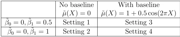
0+ ˜β1X), where g(s) = 1/{1 + exp(−s)}. Y is generated from a normal distribution with mean m(A, X) and standard deviation 0.5, where m(A, X) = ˜µ(X)−10{A−πopt_(X)}2_{. We use two} different baseline functions for ˜µ(X) and two different sets of ( ˜β0,β˜1) as shown in Table 2.1. The sample sizes are n= 400 and n = 800 and each setting is replicated 500 times.

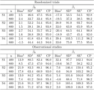
The average bias and the standard deviation of the estimated parameters from 500 simulations are summarized in the first half of Table 2.2. The estimated parameters were close to the true parameters. The third column shows the average of the standard errors estimated with the covariance function formula derived in Theorem 2.2 (see Section 2.9). 95% confidence intervals were calculated with the estimated standard errors. The coverage probabilities are shown in the table. From the result, we can see that the bias and standard deviation of the estimated parameters decreased with larger sample sizes. The coverage probabilities of the confidence intervals were close to 95%, supporting the convergence results given in Section 2.5.

We also study the performance of our method when the training data are from observational studies, where the doses given to the patients may depend on the covariates X. The simulation settings are the same as settings 1–4 except that A is generated from the distribution beta

2 exp( ˜β0 + ˜β1X),2 . The results are summarized in the second half of Table 2.2. The proposed method was still capable of giving good estimates of the parameters and the coverage of the confidence intervals were close to 95%. These simulation implies that the proposed method performs well with data from both randomized trials and observational studies.

Table 2.1: Summary of simulation settings

No baseline With baseline ˜

µ(X) = 0 µ(X) = 1 + 0.5 cos(2πX˜ ) ˜

β0 = 0,β˜1 = 0.5 Setting 1 Setting 3 ˜

β0 = 0,β˜1 = 1 Setting 2 Setting 4

(35)

Table 2.2: Simulation results from 500 replicates for randomized trials and observational studies.

Randomized trials ˜

β0 β˜1

n Bias1 SD1 SE1 CP Bias1 SD1 SE1 CP S1 400 2.5 46.6 47.5 95.6 -17.3 53.5 54.5 92.8

800 2.4 33.7 33.4 95.8 -19.5 37.3 38.5 90.2 S2 400 2.1 52.2 54.4 95.6 38.9 91.0 93.7 94.6 800 1.5 39.1 38.1 93.8 33.0 63.0 65.9 95.8 S3 400 2.7 54.1 55.7 95.2 -20.4 64.5 64.1 90.8 800 1.6 38.8 39.3 95.0 -18.9 43.7 45.4 92.0 S4 400 2.4 61.8 63.4 95.4 39.4 103.5 111.2 96.2 800 -1.5 44.4 44.3 94.6 33.6 75.0 77.5 95.6

Observational studies ˜

β0 β˜1

n Bias1 _SD1 _SE1 _CP _Bias1 _SD1 _SE1 _CP S1 400 13.9 80.5 82.4 96.0 32.4 97.7 102.1 94.6

800 8.5 47.3 47.0 94.6 -19.6 56.7 58.2 92.2 S2 400 21.9 83.3 88.1 96.4 7.6 146.4 150.4 95.2 800 17.8 63.4 60.9 93.0 0.6 94.0 103.2 98.2 S3 400 13.0 84.2 85.4 95.6 5.4 101.6 104.6 95.0 800 7.4 61.2 58.6 93.4 -4.6 68.4 71.8 96.2 S4 400 21.6 91.3 97.1 96.2 5.0 165.4 169.3 95.8 800 20.3 71.2 67.6 93.2 2.0 109.0 116.8 97.0

1_{Note: These columns are in 10}−3_scale

2_{Note: SD refers to the standard deviation of the estimated parameters}

from 500 replicates, SE refers to the mean of the estimated standard errors calculated by our covariance function, CP refers to the coverage probability of the 95% confidence intervals calculated using the estimated standard errors.

(36)

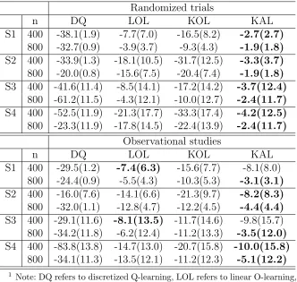
Table 2.3: Value estimate V(ˆπ) from 500 simulations in settings 1-4 Randomized trials

n DQ LOL KOL KAL

S1 400 -38.1(1.9) -7.7(7.0) -16.5(8.2) -2.7(2.7)

800 -32.7(0.9) -3.9(3.7) -9.3(4.3) -1.9(1.8)

S2 400 -33.9(1.3) -18.1(10.5) -31.7(12.5) -3.3(3.7)

800 -20.0(0.8) -15.6(7.5) -20.4(7.4) -1.9(1.8)

S3 400 -41.6(11.4) -8.5(14.1) -17.2(14.2) -3.7(12.4)

800 -61.2(11.5) -4.3(12.1) -10.0(12.7) -2.4(11.7)

S4 400 -52.5(11.9) -21.3(17.7) -33.3(17.4) -4.2(12.5)

800 -23.3(11.9) -17.8(14.5) -22.4(13.9) -2.4(11.7)

Observational studies

n DQ LOL KOL KAL

S1 400 -29.5(1.2) -7.4(6.3) -15.6(7.7) -8.1(8.0) 800 -24.4(0.9) -5.5(4.3) -10.3(5.3) -3.1(3.1)

S2 400 -16.0(7.6) -14.1(6.6) -21.3(9.7) -8.2(8.3)

800 -32.0(1.1) -12.8(4.7) -12.2(4.5) -4.4(4.4)

S3 400 -29.1(11.6) -8.1(13.5) -11.7(14.6) -9.8(15.7) 800 -34.2(11.8) -6.2(12.4) -11.2(13.3) -3.5(12.0)

S4 400 -83.8(13.8) -14.7(13.0) -20.7(15.8) -10.0(15.8)

800 -34.1(11.3) -13.5(12.1) -11.2(12.3) -5.1(12.2)

1 _{Note: DQ refers to discretized Q-learning, LOL refers to linear O-learning,}

KOL refers to kernel based O-learning, KAL refers to kernel assisted learning.

2 _{All columns are in 10}−3_{scale. For settings 3 and 4, the numbers in the}

(37)

kernel based O-learning (KOL) proposed in Chen et al. (2016) and a discretized dose rule estimated using Q-learning. For discretized Q-learning, we divide the safe dose range into 10 equally spaced intervals: A = A1 ∪...∪ A10 and create an indicator variable for each of the dose intervals I = (I1, I2, ..., I10), where Ij = I(A ∈ Aj), j = 1, . . . .,10.

The covariates included in the regression models are (X, X2_{, I, IX, IX}2_{). To this end, an} optimal dose range is selected for each individual and the middle point of the selected interval is suggested to the patient. The results from 500 replicates are summarized in Table 2.3. Each column is the average value function of the dose rule estimated by the corresponding method. The value function is evaluated at a testing dataset. The numbers in the parentheses are the standard deviation of the estimated value functions. From Table 2.3, we see that the proposed method performed the best under most settings. In the simulation for observational studies, O-learning performed the best when the sample size was small. However, the proposed method performed comparatively well and performed better as the sample size increased. The discretized Q-learning method did not provide a good dose suggestion in this case.

We then apply our method to a slightly more complicated setting with 3 covariates.X1, X2,X3 are generated independently from a uniform(−1,1) and A follows a uniform(0,2) and is independent of X. Y is generated as follows:

Setting 5: ˜

β =c(1,0.5,0.5,0), X = (1, X1, X2, X3)T, πopt(X) = ˜βTX,

m(A, X) = 8 + 4X1−2X2 −2X3−25× {A−πopt(X)}2, Y ∼N{m(A, X),1}. The rate of the bandwidths are chosen to be n−1/8_.

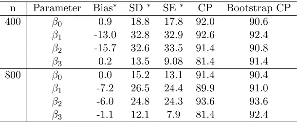
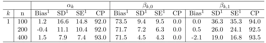
The results of setting 5 are summarized in Table 2.4. The average bias of the estimated parameters was small and decreased as the sample size increased. However, the estimated standard error was not stable with increased number of parameters. Thus, the coverage probabilities of the 95% confidence intervals were inaccurate for some of the parameters. According to Horowitz (2001), the bootstrap can provide refinements to the estimation of standard deviations for kernel density estimation. Therefore, we estimate the standard error using the bootstrap with 100 repetitions and calculate the bootstrap confidence interval. It appears that the bootstrap confidence intervals were more stable. The coverage of the bootstrap confidence intervals were close to 95%.

(38)

function of the dose rule estimated by the corresponding method. The value function is evaluated at a testing dataset. The numbers in the parentheses are the standard deviation of the estimated value functions. From Table 2.5, we see that linear O-learning performed comparatively well with our kernel assisted learning method (KAL). The discretized Q-learning method did not provide a good dose suggestion in this case.

Table 2.4: Average ˆβn from 500 replicates for setting 5

n Parameter Bias∗ SD∗ SE ∗ CP Bootstrap CP

400 β0 0.9 18.8 17.8 92.0 90.6

β1 -13.0 32.8 32.9 92.6 92.4 β2 -15.7 32.6 33.5 91.4 90.8 β3 0.2 13.5 9.08 81.4 91.4

800 β0 0.0 15.2 13.1 91.4 90.4

β1 -7.2 26.5 24.4 89.9 91.0 β2 -6.0 24.8 24.3 93.6 93.6 β3 -1.1 12.1 7.9 81.4 92.4

1 _{Note: * columns are in 10}−3 _scale

2 _{Note: SD refers to the standard deviation of the estimated}

param-eters from 500 replicates, SE refers to the mean of the estimated standard error calculated by our covariance function, CP refers to the coverage probability of the 95% confidence intervals calculated using the estimated standard errors, Bootstrap CP refers to the coverage probability of the 95% confidence intervals calculated using the bootstrap estimated standard errors.

3 _{Note: The worst case Monte Carlo standard error for proportions is}

1.8%.

Table 2.5: Value estimate V(ˆπ) from 500 simulations in setting 5

Discretized Q LOL KOL KAL

N=400 5.66(0.32) 7.85(0.14) 5.77(0.15) 7.96(0.10) N=800 5.76(0.27) 7.92(0.11) 5.82(0.14) 7.97(0.09)

1 _{Note: Discretized Q refers to discretized Q-learning, LOL refers to}

(39)

2.7 Warfarin Data Analysis

Warfarin is a widely used anticoagulant for prevention of thrombosis and thromboembolism. Although highly efficacious, dosing for warfarin is known to be challenging because of the narrow therapeutic index and the large variability among patients (Johnson et al. 2011). Overdosing of warfarin leads to bleeding and underdosing diminishes the efficacy of the medication. The international normalized ratio (INR) measures the clotting tendency of the blood. An INR between 2–3 is considered to be safe and efficacious for patients.

Typically, the warfarin dosage is decided empirically: an initial dose is given based on the population average, and adjustments are made in the subsequent weeks while the INR of the patient is being tracked. A stable dose is decided in the end to achieve an INR of 2–3 (Johnson et al. 2011). The dosing process may take weeks to months, during which the patient is constantly at risk of bleeding or under-dosing. Therefore, a quantitative method for warfarin dosing will greatly decrease the time, cost and risks for patients.

The following analysis uses the warfarin dataset collected by Consortium (2009). In the original paper, a linear regression was used to predict the stable dose using clinical results and pharmacogenetic information, including age, weight, height, gender, race, two kinds of medications (Cytochrom P450 and Amiodarone), and two genotypes (CYP2C9 genotype and VKORC1 genotype). This prediction method is based on the assumption that the stable doses received by the patients are optimal. However, later studies showed that the suggested doses by the International Warfarin Pharmacogenetic Consortium were suboptimal for elderly people, implying that the optimal dose assumption might not be valid (Chen et al. 2016).

We apply the proposed method to this dataset to estimate the optimal individualized dose rule for warfarin. Instead of using only the data of the patients with stablized INR, we include all patients who received weekly doses between 6 mg to 95 mg. The medication information is missing for half of the observations and is therefore excluded from our analysis. Observations which are missing in the other variables are removed from the dataset, resulting in a total of 3567 patients. The outcome variable is defined as Yi =−(INRi−2.5)2 for the i th observation. Stratification of the categorical variables

is needed for the kernel density estimation. In order to ensure that there are enough observations in each stratified group, we consider only categorical variables that are distributed comparatively even among different groups. In our analysis, we use three variables: height, gender and the indicator variable for VKORC1 of type AG. Before we apply the proposed the method, we normalize all the variables byXi,j = (Xi,j−X¯j)/sd(Xj),

(40)

the j-th variable.

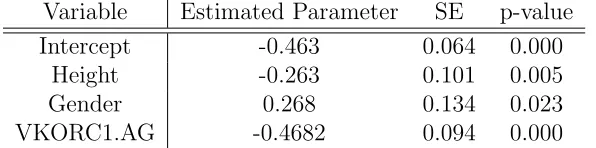
The estimation results are shown in Table 2.6. The p-value is obtained for each of the parameters. The result implied that the optimal dose for male is higher than the optimal dose for female given all the other variables are the same. It was also implied that the patients with genotype VKORC1=AG need higher doses than the patients with VKORC16= AG. We use the same variables and compare our method with O-learning and the discretized Q-learning method. For the discretized Q-learning method, we also divide the dose range into 10 equally spaced intervals. The suggested doses by the three methods are shown in Fig. 2.2. The result shows a tendency of the discretized Q-learning to suggest extreme doses, which is not ideal in real application. This might be due to the fact that the higher dose intervals contain small numbers of observations, and thus the estimated models are dominated by a few subjects.

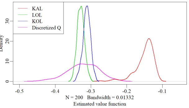
To evaluate the estimated dose rules of these methods, we randomly take two thirds of the data as training data and the rest of the data as testing data. The optimal individualized dose rule is estimated with the training data. The value function of the suggested individualized dose rule V(ˆπ) is estimated with the average of the Nadaraya Watson estimator for E{Y |X, A= ˆπ(X)}in the testing dataset. The tuning parameters for the Nadaray-Watson estimators are taken ashx = 1.25sd(X)n

−1/4.5

test andha= 1.75sd(A)n

−1/4.5 test , where ntest= 1189 is the size of the testing dataset. The process is repeated 200 times. The distribution of the estimated value of the suggested dose is shown in Fig. 2.3. The suggested individualized dose rule with our proposed method lead to better expected outcomes in the population compared to the other methods. The performance of the discretized Q-learning method was not stable as shown in the result. However, this result was only based on the three variables selected, while in reality, the two medications (Cytochrome P450 enzyme and Amiodarone) and the genotype CYP2C9 are also of significant importance in warfarin dosing. The computation complexity of our proposed method restricted its capability of handling higher dimensional problems.

Table 2.6: Estimated ˆβ with warfarin data with kernel assisted learning Variable Estimated Parameter SE p-value

Intercept -0.463 0.064 0.000

Height -0.263 0.101 0.005

Gender 0.268 0.134 0.023

(41)

Figure 2.1: Distribution of the variables in the warfarin dataset.

(a)

(b)

(42)

Figure 2.3: Empirical distribution of the estimated value function over 200 repetitions for the warfarin dataset. The green line denotes the result from linear O-learning. The blue line denotes the result from kernel based O-learning. The red line denotes the result from kernel assisted learning. The pink line denotes the result from discretized Q-learning.

2.8 Discussion and Conclusion

The proposed kernel assisted learning method for estimating the optimal individualized dose rule provides the possibility of conducting statistical inference with estimated dose rules, thus providing insights on the importance of the covariates in the dosing process. In our simulation settings, the proposed method was capable of identifying the optimal individualized dose rule when the optimal dose rule was inside the prespecified class of rules. In the warfarin dosing case, based on the three covariates selected, the suggested dose appeared to lead to better expected clinical result compared to the other methods. The proposed method has several possible extensions. Notice that the form of the prespecified rule class can be extended to a link function with a nonlinear predictor g{Ψ(X)T_β} _{where Ψ(·) =}_{Ψ

1(·), ...,Ψc(·)}T are some prespecified basic spline functions

and β∈_Rc _{. The accuracy of the approximated value function might also be improved}

by extending the multivariate kernel Kq(x/hx)/hx to |H|−1/2Kq(H−1/2x) (Duong and

Hazelton 2005).

One weakness of the proposed method is that the accuracy of the estimated value function is sensitive to the choice of bandwidth. The kernel density estimator in the denominator of Mn(β) might lead to large bias when the bandwidths are not properly

(43)

the mean squared error of the Nadaraya-Watson estimator. However, due to the complex form ofMn(β), this method might not be optimal when the dimension of the covariates

(44)

2.9 Proof and Technical Details

2.9.1 Proof of Theorem 2.1

We first prove the uniform convergence of Mn(β) to M(β). For simplicity of notation,

let’s define:

mx(x, a) =∂m(x, a)/∂x, m2x(x, a) =∂m2(x, a)/∂x, m2a(x, a) =∂m2(x, a)/∂a. Simi-larly, fa(x, a) =∂fX,A(x, a)/∂a,fx(x, a) =∂fX,A(x, a)/∂x. We write Mn(β) as

Mn(β) =

Z

x

An(x;β)

Bn(x;β)

Cn(x)dx,

where

An(x;β) =

1 n n X i=1 Yi 1 hqx

Kq(

x−Xi

hx

) 1 ha

Kg(β

T_x)₋_A i

ha

,

Bn(x;β) =

1 n n X i=1 1 hqx

Kq(

x−Xi

hx

) 1 ha

Kg(β

T_x)₋_A i

ha

,

Cn(x) =

1 n n X i=1 1 hqx

Kq(

x−Xi

hx

).

Notice that M(β) can be written as

M(β) =

Z

x

A(x;β)

B(x;β)C(β)dx,

where A(x;β) = m{x, g(βT_x)}f

X,A{x, g(βTx)}, B(x;β) = fX,A{x, g(βTx)} and C(x) =

fX(x). Thus,

sup

β

Mn(β)−M(β) = sup β Z x

nA_n(x;β)

Bn(x;β)

Cn(x)−

A(x;β) B(x;β)C(x)

o dx ≤sup β Z x

nA_n(x;β)

Bn(x;β)

− A(x;β) B(x;β)

o

Cn(x)dx

+ sup β Z x A(x;β) B(x;β) n

Cn(x)−C(x)

o dx ≤sup a,x

A∗_n(x, a) B∗

n(x, a)

− A

∗_{(x, a)}

B∗_{(x, a)}

nZ

x

Cn(x)dx

o

+ sup

a,x

|m x, a)|n

Z

x

Cn(x)−C(x) dx

Statistical Methods for Optimal Dose Finding.

ABSTRACT

DEDICATION

ACKNOWLEDGEMENTS

TABLE OF CONTENTS

LIST OF TABLES

LIST OF FIGURES

CHAPTER

1

INTRODUCTION

1.1

Motivation

1.2

Outline

1.3

Notations

CHAPTER

2

KERNEL ASSISTED LEARNING FOR

SINGLE-STAGE PERSONALIZED DOSE

FINDING

2.1

Introduction

2.2

Problem Setting

2.3

Literature Review

2.3.1

Methods for Finding Discrete Optimal Treatment Rules

2.3.2

Methods for Finding Optimal Dose Rules

2.4

Kernel Assisted Learning

2.4.1

Method

2.4.2

Computational Details

2.5

Theoretical Results

2.6

Simulation Studies

2.7

Warfarin Data Analysis

2.8

Discussion and Conclusion

2.9

Proof and Technical Details

2.9.1

Proof of Theorem 2.1