ABSTRACT
FAN, AILIN. New Statistical Methods for Precision Medicine: Variable Selection for Optimal Dynamic Treatment Regimes and Subgroup Detection. (Under the direction of Dr. Wenbin Lu and Dr. Rui Song.)
Due to patients’ heterogeneity and a growing number of specifically targeted treatments, precision medicine draws attentions for customization of therapies and medical decisions for individual patient. In this dissertation, we investigate statistical methods to address two prob-lems in precision medicine. The first problem is variable selection for optimal dynamic treatment regime. Variable selection is gaining more attention because it plays an important role in deriv-ing practical and reliable optimal treatment regimes, especially when there are a large number of predictors. The second problem is subgroup detection of patients with enhanced treatment effects. By assessing heterogeneous treatment effects based on a variety of covariates, subgroup detection helps narrow down the target population of a treatment.
In Chapter 2, we develop a sequential advantage selection method for variable selection for optimal treatment regime. Variables that have qualitative interactions with treatment are of clinical importance for treatment decision-making. A qualitative interaction of a variable with treatment arises when the treatment effect changes direction as the value of the variable varies. Our sequential advantage selection method sequentially selects variables with a qualitative interaction and can be applied in multiple-decision-point settings. Numerical studies suggest that the proposed method is useful in identifying important variables under various underlying true models.
© Copyright 2016 by Ailin Fan
New Statistical Methods for Precision Medicine: Variable Selection for Optimal Dynamic Treatment Regimes and Subgroup Detection
by Ailin Fan
A dissertation submitted to the Graduate Faculty of North Carolina State University
in partial fulfillment of the requirements for the Degree of
Doctor of Philosophy
Statistics
Raleigh, North Carolina 2016
APPROVED BY:
Dr. Howard D. Bondell Dr. Eric B. Laber
Dr. Wenbin Lu
Co-chair of Advisory Committee
Dr. Rui Song
DEDICATION
BIOGRAPHY
ACKNOWLEDGEMENTS
I would first like to express my deepest gratitude to my advisors, Dr. Wenbin Lu and Dr. Rui Song, for their excellent guidance and enormous support. They help me get started in statistical research, and show integrity and discretion in every step of research work. I have the highest regard for their passion in research and broad knowledge in statistics. They are able to express wonderful ideas in brief words, and are always accommodating and generous with their time. I could not have chosen two better mentors to guide me through my statistical research, and this dissertation would not be possible without their inspiration and encouragement.
I would also like to thank Dr. Howard Bondell and Dr. Eric Laber for serving on my dissertation committee. They have provided constructive comments that help me improve my work presented in this dissertation. I also thank Dr. James Wilson, who agreed to serve on my committee as the graduate school representative out of his busy schedule.
I appreciate the study opportunity provided by the Department of Statistics at North Car-olina State University. I am grateful for all the faculty members for offering great courses on various topics that broaden my knowledge of statistics. I thank Dr. Daowen Zhang for being my academic advisor during my first two years’ study. His valuable guidance helped me have a bet-ter plan of my Ph.D. study and research. I also enjoyed random talks with Dr. John Monahan and Dr. Dennis Boos in the hallways. I thank Dr. Charles Smith for his snacks and toys when I stay late in SAS Hall. I also thank DGPs and the department staff for their patience when I bug them with questions on requirements of the program. Special thanks to all my friends who share laughs and tears with me in these years. You have made graduate school enjoyable and memorable.
he showed me how to collaborate and communicate with scientists from other fields of study, and made my experience at GSK very fruitful. Alex and Rain were energetic and inspiring, and gave me valuable advices on how to be a good statistical consultant and a good presenter when I was at SAS. I appreciate all their mentorship that sharpened my career aspirations.
TABLE OF CONTENTS
LIST OF TABLES . . . .viii
LIST OF FIGURES . . . ix
Chapter 1 INTRODUCTION . . . 1
Chapter 2 VARIABLE SELECTION FOR OPTIMAL TREATMENT REGIME 5 2.1 Introduction . . . 5
2.2 Overview for Dynamic Treatment Regime . . . 8
2.2.1 Data Structure . . . 8
2.2.2 Potential Outcomes and Assumptions . . . 9
2.2.3 Optimal Dynamic Treatment Regimes . . . 11
2.3 S-Score Ranking . . . 12
2.4 Sequential Advantage Selection . . . 14
2.4.1 Sequential Advantage . . . 14
2.4.2 Sequential Advantage Selection Algorithm . . . 15
2.4.3 Extension to Multi-Stage Treatment Decisions . . . 16
2.5 Simulation Studies . . . 18
2.5.1 Single-Stage Treatment Decision Study . . . 18
2.5.2 Multi-Stage Treatment Decisions Study . . . 22
2.6 Application to STAR*D Study . . . 25
2.7 Discussion . . . 28
Chapter 3 PENALIZED A-LEARNING FOR OPTIMAL TREATMENT DE-CISIONS WITH NP-DIMENSIONALITY . . . 37
3.1 Introduction . . . 37
3.2 Penalized A-Learning . . . 39
3.3 Some Implementation Issues . . . 43
3.4 Simulation Studies . . . 44
3.4.1 Settings . . . 44
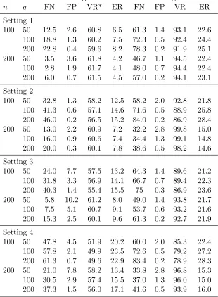
3.4.2 Results . . . 46
3.5 Application to STAR*D Study . . . 48
Chapter 4 CHANGE-PLANE ANALYSIS FOR SUBGROUP DETECTION AND SAMPLE SIZE CALCULATION . . . 53
4.1 Introduction . . . 53
4.2 Change-Plane Analysis . . . 56
4.2.1 The Proposed Model . . . 56
4.2.2 A Doubly-Robust Test . . . 57
4.2.3 Asymptotic Distributions ofTn . . . 59
4.3 Sample Size Calculation . . . 62
4.4.1 Test and Estimation . . . 63
4.4.2 Sample Size Calculation Examples . . . 67
4.5 Application to AIDS Data . . . 69
4.6 Discussion . . . 70
BIBLIOGRAPHY . . . 78
LIST OF TABLES
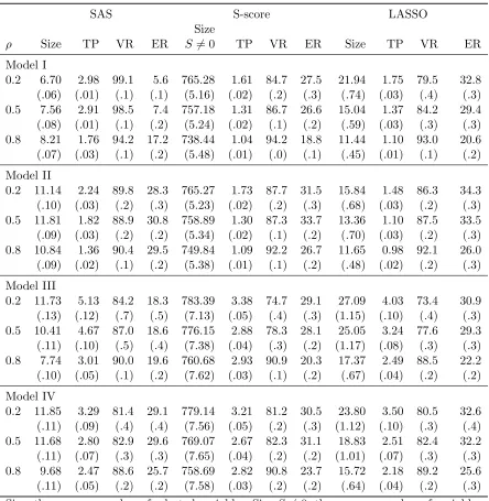
Table 2.1 Simulation results of sequential advantage selection (SAS), S-score and LASSO methods in the single-stage treatment decision study. . . 31 Table 2.2 Optimal Treatment Regimes and Corresponding Important Variables in
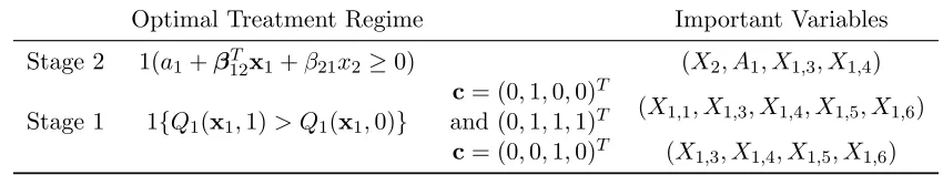
Multi-Stage Simulation Study . . . 32 Table 2.3 Simulation Results of SAS-MTD method for Two-Stage Treatment Decisions
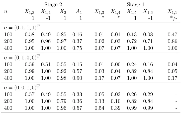
Study. . . 32 Table 2.4 Proportion of Each Important Variable Being Selected at Stage 2 and Stage 1. 34 Table 2.5 List of covariates used in the analysis of STAR*D study. . . 35 Table 2.6 Estimated Values of Different Treatment Regimes and Confidence Intervals
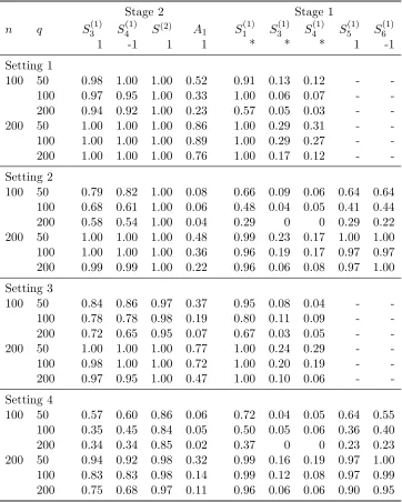
for the Differences of Values. . . 36 Table 3.1 Simulation Settings. . . 50 Table 3.2 Variable Selection Simulation Results (%). . . 51 Table 3.3 Proportion of Each Important Variable Being Selected at Stage 2 and Stage 1. 52 Table 4.1 Type I errors of the proposed test based on resampling. (Corresponding
standard errors for type I errors with size 0.05 and 0.1 are 0.003 and 0.004.) 72 Table 4.2 Power (%) of the proposed test at 0.05 and 0.1 levels. (Standard errors are
shown in parenthesis.) . . . 73 Table 4.3 Misclassification rate (%) of identified subgroup based on estimated
change-plane parameterθ. (Standard errors are shown in parentheses.) . . . 75 Table 4.4 Average timing performance (in seconds). . . 75 Table 4.5 Type I error and power (%) of the EM test (Shen and He, 2015) and our
method for B-Model I at 0.05 and 0.1 levels. (Standard errors are shown in parenthesis.) . . . 75 Table 4.6 Misclassification rate (%) of identified subgroup based on Zhao et al. (2013)
with different cut-off pointc such that dAD(c) =τ and our method. Results are summarized under scenarios with P-Model I and B-Model I/II/III. . . 76 Table 4.7 Results for sample size calculation. Here,nis the required sample size given
by our procedure. Empirical power of the test with the calculated sample size is reported based on 1000 data replications. . . 76 Table 4.8 Results for sample size calculation based on the method in Brookes et al.
(2004) and Borm et al. (2007). Here,nis the required sample size. Empirical power of the test with the calculated sample size is reported based on 1000 data replications. . . 76 Table 4.9 Required sample sizes for detecting a subgroup with an enhanced treatment
LIST OF FIGURES
Figure 2.1 Plots of the marginal interaction of covariatesX1,X9, and X10 with treat-ment (triangles are for treattreat-ment 1, and circles are for treattreat-ment 0). The fitted lines for treatment 1 (dashed) and treatment 0 (dotted) are from sim-ple linear regression. The left panel is for ρ = 0.2; the right panel is for
ρ= 0.8. . . 30 Figure 2.2 Solution paths of sequential advantage selection (SAS, solid line), S-score
Chapter 1
INTRODUCTION
Precision medicine is emerging as a new medical paradigm for treatment that is tailored to an individual’s genes, environment and lifestyle. It is of interest to develop statistical methods used in discovery and characterization of heterogeneity of subject responses to treatments. We tackle the problems in precision medicine applications under two frameworks: the first framework is to find the right treatment for each subject, which is conceptualized as optimal dynamic treatment regime; the second framework is to find the right subject for a given treatment, which is conceptualized as subgroup detection.
(Fava et al., 2003; Rush et al., 2004). A large number of works have been developed to derive optimal dynamic treatment regimes based on data from clinical trials and observational studies. For example, marginal structure models (Robins, 1997; Murphy et al., 2001) allow estimation of the mean response under a dynamic treatment regime. Q-learning (Watkins, 1989; Watkins and Dayan, 1992; Murphy, 2005; Zhao et al., 2011; Chakraborty et al., 2010; Song et al., 2015) and A-learning (Murphy, 2003; Robins, 2004) are two popular backward induction methods for deriving optimal dynamic treatment regimes: the former builds regression models for the so-called Q functions while the latter is based on modeling contrast functions. In particular, A-learning has the double robustness property, i.e. when either the baseline mean function or the propensity score model is correctly specified, the resulting A-learning estimating equation for the contrast function is consistent.
A major challenge in deriving an optimal dynamic treatment regime arises when an ex-traordinary large number of prognostic factors are available, but not all of them are necessary for making treatment decision. This makes variable selection an emerging need in personalized medicine. Most existing variable selection techniques focus on selecting variables that are im-portant for prediction. With such methods, some variables that are poor in prediction but are critical for treatment decision-making may be ignored.
qualitative interactions. To select the best candidate subset of variables for decision-making, we also propose a BIC-type criterion that is based on the sequential advantage. We evaluated the empirical performance of the proposed method in both single-decision-point and multiple-decision-point settings, as well as in an application to depression data from a clinical trial. In Chapter 3, we propose a penalized A-learning method for deriving the optimal dynamic treatment regime when the number of covariates is of the non-polynomial order of the sample size. To preserve the double robustness property of the A-learning method, we adopt the Dantzig selector which directly penalizes the A-leaning estimating equations. Empirical performance of the proposed approach is evaluated by simulations and illustrated with an application to a data from the STAR*D study.
likelihood-based test for the existence of a subgroup.
Chapter 2
VARIABLE SELECTION FOR
OPTIMAL TREATMENT REGIME
2.1
Introduction
Personalized medicine is emerging as a new strategy for treatment that takes individual het-erogeneity in background characteristics, clinical measurements, and genetic information into consideration. In this paradigm, treatment duration, dose, and type are adjusted over time and are tailored according to an individual’s information with the aim of optimizing the effective-ness of treatment. This approach is different from the traditional “one-size-fits-all” treatment, which ignores the long-term benefits and individual heterogeneities. Great interest lies in find-ing optimal treatment regimes based on data from clinical trials and observational studies (e.g. Murphy, 2003; Robins, 2004; Moodie et al., 2007).
collect all of this information in clinical practice, and redundancy in covariate information may impair the accuracy of optimal treatment decisions as well as its interpretation. Thus, a natural problem that arises in the estimation of optimal treatment regimes is how to identify the important covariates for treatment decision making.
Although variable selection is an important area in modern statistical research, current vari-able selection techniques mainly focus on selecting varivari-ables for prediction. Such approaches may not be able to adequately predict the interactions of variables with treatment and thus may ne-glect variables that are vital for decision making. In medical decision-making settings, variables that have qualitative interactions with treatments are clinically important (Peto, 1982). These variables are called prescriptive variables, which help prescribe the optimal treatment regimes. These variables should be distinguished from predictive variables, which help to increase pre-diction accuracy.
measure that characterizes the qualitative interaction of an individual variable with treatment, namely the S-score. Then, a hybrid algorithm that combines S-score ranking and weighted LASSO was used to select variables for treatment decision-making.
Our work was motivated from the Sequenced Treatment Alternatives to Relieve Depression (STAR*D) study (Fava et al., 2003; Rush et al., 2004). The STAR*D study was a sequential, multiple-assignment, randomized trial (SMART, see Murphy (2005); Qian et al. (2013)) for patients with non-psychotic major depressive disorder. This study aimed to determine which antidepressant medications, in what order, and what combination, should be given to patients to yield the optimal treatment effect. A large number of covariates were collected at baseline, such as patient demographic characteristics and medical history. In addition, several intermediate medical measurements were taken to assist in treatment decision making at the second or higher treatment decision points. It is hard to select covariates useful for making decisions from such a large number of covariates based on experts’ opinions only. Thus, variable selection is crucial for deriving the optimal treatment regimes in the STAR*D trial.
unimportant. The proposed method has satisfactory performance in each stage of dynamic treat-ment regimes. Because the proposed method starts from the null model, the impletreat-mentation is feasible in high-dimensional settings provided that the true model is sufficiently sparse.
The remainder of the chapter is organized as follows. In Section 2.2, we introduce the framework for deriving optimal dynamic treatment regimes. In Section 2.3, S-score ranking for selecting prescriptive variables is introduced. Section 2.4 provides the proposed sequential advantage selection method for variable selection in optimal treatment decision-making. We demonstrate the method’s performance in Section 2.5 by simulation studies in various scenarios and illustrate the method using data from the STAR*D clinical trial in Section 2.6.
2.2
Overview for Dynamic Treatment Regime
Potential outcome model is the framework for developing optimal dynamic treatment regimes. It was first introduced by Neyman et al. (1990) to analyze the causal effect of time-independent treatments in randomized studies. Rubin (1978) extended Neyman’s work to the analysis of causal effects of time-independent treatments from observational data. Robins (1986) proposed a formal theory of causal inference based on their works, which extended Rubin’s “point treat-ment” theory to longitudinal studies with direct and indirect effects and time-varying treatments and confounder. In this section, we will first introduce the notation and data structures for the dynamic treatment regime problem, then potential outcome models and assumptions will be provided to make causal inference based on the observed data. Lastly, the optimal dynamic treatment regimes will be defined using the potential outcomes.
2.2.1 Data Structure
may be fixed or random, depending on the characteristic of the treatment. The data for a single individual can be summarized as a time-ordered sequence of variables
(X1, A1, ...,XK, AK, Y),
whereX1, ...,XK are covariate information measured prior to treatment at the beginning of each time pointt1, .., tK, whose possible value sets are X1, ...,XK; andA1, ..., AK are the treatments given at each time pointt1, ..., tK among a possible set of treatments denote byA1, ...,AK. The outcome of interest isY with larger values indicating better response. The setsXk(k= 1, ..., K) and Ak (k= 1, ..., K) could be either finite or infinite, and both can be multidimensional.
Overbar notation is used to denote the history of time-dependent variables. That is, ¯XK = (X1, ...,XK),A¯k = (A1, ..., Ak), k = 1,2, ..., K −1, and ¯X = (X1, ..,XK),A¯ = (A1, ..., AK). Upper case Roman letters denote random variables and lower case Roman letters denote the realizations of the random variables. Then the observed data are summarized as
Oi = (X1i, A1i, ..., XKi, AKi, Yi), i= 1, ..., n,
whereiindicates theith individual in the sample.{Oi, i= 1, .., n}are independent and identi-cally distributed across i.
2.2.2 Potential Outcomes and Assumptions
of all potential outcomes is defined as
W =
{X1,X∗2(a1),X∗3(¯a2), ...,X∗K(¯aK−1), Y∗(¯a)}, fora1 ∈ A1, ...,a¯K−1 ∈A¯K−1,a¯∈A¯ ,
where X∗k(¯ak−1), k = 2, ..., K are potential intermediate covariates that would accrue between
tk−1andtkgiven the treatment history ¯ak−1 (k= 2, ..., K) andY∗(¯a) is potential final response that would result if treated according to ¯aK. Note that the potential outcomes are defined for all possible treatments. They are also named as counter-factual variables because only the outcomes corresponding to the treatment regime given to the individual could be observed in reality; the other potential outcomes are corresponding to hypothetical values if the individual actually receives a treatment different from the one considered.
Suppose we have a treatment ¯a which is corresponding to no interventions at all decision points, the causal effect of another treatment ¯a0 on the final outcomes at the individual level can be written asY∗(¯a0)−Y∗(¯a). Because only the potential outcomes at the particular treat-ment regime that is given to the individual can be observed, it is not possible to estimate the individual causal treatment effect. However, the treatment causal effect at population level, which isE(Y∗(¯a0)−Y∗(¯a)), is possible to be estimated under the following assumptions on the potential outcomes:
(1) Stable Unit Treatment Value Assumption (SUTVA): an individual’s outcome is the same as the potential outcome for the assigned treatment, and is not influenced by other indi-vidual’s treatment allocation (Rubin, 1978). That is, if an individual receives treatment
¯
A, we have Xk = X∗k( ¯Ak−1) = P¯ak−1∈A¯k−1X
∗
k(¯ak−1)I( ¯Ak−1 = ¯ak−1), k = 2, ..., K, and
Y =Y∗( ¯A) =P ¯
a∈A¯Y∗(¯a)I( ¯A= ¯a).
holds for k= 1, ..., K, whereA0 is null.
The SUTVA is usually reasonable but cannot be verified generally, such as in a vaccine intervention situation, where the individual’s outcome is clearly affected by the treatments of others. In epidemiology, the confounders are referred to as the variables that may be related both to the outcomes and the individuals who may get treatment. The no unmeasured con-founders assumption states that treatment assignment is based on past recorded information only. This assumption holds in a sequentially randomized experiment, but may be questionable in an observational study. Under these two assumptions, the average treatment causal effect
E(Y∗(¯a0)−Y∗(¯a)) could be estimated by ˆE(Y|A¯= ¯a0)−Eˆ(Y|A¯= ¯a), which only depends on the observed data.
2.2.3 Optimal Dynamic Treatment Regimes
A dynamic treatment regime is a set of rules that shows how to treat an individual over time based on the past information. We denote the dynamic treatment regime as d= (d1, ..., dK), wheredk: Γk→ Akis a map of current available information at timetkto the possible treatment decisions that could be made attk. Here Γk={(¯xk,a¯k−1)∈X¯k×A¯k−1}is the set of historical information including covariates and treatments. The goal is to find a treatment regime that maximizesE(Y∗(d)), the mean potential outcome of a population if all the individuals are given treatments indicated by the treatment regime d.
To find the optimal dynamic treatment regime, we need to derive the distribution of the potential outcomes {X1,X∗2(d), ...,XK∗(d), Y∗(d)} based on the distribution of the ob-served data {O1, ..., On}. The two key assumptions in section 2.2.2 are required to estimate the effect of a dynamic regime. Under these assumptions, the joint density of the poten-tial outcomes{X1,X∗2(d), ...,XK∗(d), Y∗(d)} for any treatment regimedcould be obtained as
PX1,...,XK∗(d),Y∗(d)(X1, ...,XK, y) =pX
responseE(Y∗(d)) could be expressed as:
EhY∗(¯a)a1=d1(X1),...,a
K=dK{X¯K(¯aK−1),¯aK−1}
i
=E[E[· · ·E[Y|X¯K,A¯K−1, AK =dK]· · · |X1, A1 =d1]]. (2.1) This is Robins’s G-computation (Robins, 1986, 1997; Gill and Robins, 2001). See Gill and Robins (2001) and Murphy (2003) for more general conditions and proofs.
Suppose the class of regimes we consider isD. To find the optimal dynamic treatment regime amongD, the treatments indicated by regimed∈ Dshould be represented by the observed data. This requirement leads to another important assumption for indicating the optimal dynamic treatment regime: the positivity assumption (Robins, 1994). That is, the treatment patterns which are consistent with the regime d∈ D can occur in the longitudinal data with positive probability: PA¯
k|X¯K,A¯k−1(ak|s¯k,¯ak−1) > 0, for (¯sk,a¯k−1) satisfies PS¯k,A¯k−1(¯sk,a¯k−1) > 0 and
ak=dk(¯sk,a¯k−1), k= 1, ..., K. In practice, optimal dynamic regimes could be applied to obser-vational data or data from clinical trials. Recently, the experimental designs that are specifically suited for finding the optimal dynamic treatment regimes are of interest (Murphy, 2005; Collins et al., 2007), and the Sequential Multiple Assignment Randomized Trials (SMART, Murphy, 2005) design is widely used for constructing the optimal dynamic treatment regime (Thall et al., 2000; Rush et al., 2004; Auyeung et al., 2009; Chakraborty et al., 2010).
2.3
S-Score Ranking
characterizes the degree of qualitative interaction of a variable. For single treatment decision
A, the S-score for thejth covariate, Xj, is defined as:
Sj = n X
i=1 h
max a {
ˆ
E(Yi|Xij =xij, Ai=a)} −Eˆ(Yi|Xij =xij, Ai = ˆa) i
, (2.2)
where ˆE(Yi|Xij =xij, Ai =a) is an estimator ofE(Yi|Xij =xij, Ai =a), and ˆa= argmaxaEˆ(Y|A=
a), i.e., the treatment that leads to the largest treatment-specific mean response. The S-score is always non-negative, and a higher valued S-score indicates a greater potential for the covariate to have a qualitative interaction with treatment.
To show that the S-score captures both the magnitude of interaction and the proportion of subjects whose optimal treatment changes, we illustrate with an example. Consider the model E(Y|Xj, A) = β0 +β1Xj +β2A+β3XjA, and let ( ˆβ0,βˆ1,βˆ2,βˆ3)T denote the estimates of (β0, β1, β2, β3)T. The S-score forXj is then given by
Sj = n X
i=1
( ˆβ2+ ˆβ3xij) h
1( ˆβ2+ ˆβ3xij ≥0)−aˆ i
. (2.3)
In equation (2.3), ( ˆβ2+ ˆβ3xij) represents the magnitude of the treatment effect as a function of
Xij, and 1( ˆβ2+ ˆβ3xij ≥0)−ˆaindicates whether the optimal treatment for patient i changes given the knowledge of Xij. Therefore, both factors are reflected in the S-score.
in the weighted LASSO selection. In addition, an adjusted gain in value criterion is used to select the best subset of variables along the solution path for those selected non-zero S-scores. This hybrid algorithm helps to pick variables among the pool of variables with non-zero S-scores. Second, because the S-score evaluates each variable individually, some variables that are jointly crucial for optimal treatment decision-making may be neglected. Third, the S-score method proposed by Gunter et al. (2011) is only studied for a single-stage treatment decision. These limitations motivate us to develop a forward-selection procedure based on a modified S-score, namedsequential advantage, for selecting variables having qualitative interactions with treatment for both single-stage and multi-stage treatment decisions.
2.4
Sequential Advantage Selection
In this section, we introduce sequential advantage and describe sequential advantage selection algorithms for both single-stage and multi-stage treatment decisions.
2.4.1 Sequential Advantage
We introduce sequential advantage in a single-stage treatment decision study. LetM={j1, .., jk}
denote an arbitrary model withXj1, ..., Xjk as the selected covariates andF ={1, ..., p}denote
the full model. In addition, letXidenote the covariate for subjectiandXi(M)={Xij :j ∈ M} denote the associated covariates corresponding to model M. The sequential advantage of vari-able Xj,j∈ F \ M(k−1), is defined as:
Sj(k)=1
n
n X
i=1
max a {
ˆ
E(Y|XM(k)
j
=xiM(k)
j
, A=a)}
−Eˆ(Y|XM(k)
j
=xiM(k)
j
, A=a(k−1)opt (xiM(k−1)))
where M(k−1) ={j1, ..., jk−1} is the model selected at the (k−1)th step, M(k)j =M(k−1)∪ {j}, ˆE(Y|XM(k)
j
= xiM(k)
j
, A = a) is the estimated conditional mean response based on an assumed model with predictors XM(k)
j
and A, and a(k−1)opt (xiM(k−1)) is the optimal treatment
regime obtained based on the variables inM(k−1). In practice, a linear model with main effects of XM(k)
j
and A as well as interaction effects between XM(k)
j
and A can be used to obtain ˆ
E(Y|XM(k)
j
= xiM(k)
j
, A= a). Similarly, a(k−1)opt (xiM(k−1)) can be obtained based on the fitted
model ˆE(Y|XM(k−1) =xiM(k−1), A=a). The sequential advantage defined in (2.4) is similar to
the S-score in spirit, but represents the additional benefit of including variable Xj to improve the optimal treatment regime estimated based on previously selected variables.
2.4.2 Sequential Advantage Selection Algorithm
In this section, we propose a variable selection method based on sequential advantage in a forward selection manner. We first describe the sequential advantage selection (SAS) algorithm for selecting variables that have a qualitative interaction with treatment in a single treatment decision study, and then extend SAS to accommodate multiple treatment decisions using Q-learning in the next section. The SAS algorithm for a single-stage treatment decision is given as follows.
(i) Initialization. Set M(0) = ∅. Compute a(0)
opt = argmaxaEˆ(Y|A = a), and let S(0) = ˆ
E(Y|A=a(0)opt)−Eˆ(Y).
(ii) Sequential Advantage Selection. In the kth step (k ≥ 1), we have M(k−1). For every j ∈ F \ M(k−1), we consider candidate covariates M(k)j = M(k−1) ∪ {j} and compute the sequential advantage (2.4) corresponding to the jth covariate in the kth step. The kth variable to be selected is the one with the largest sequential advantage in this step: jk = argmaxj∈F \M(k−1){Sj(k)}. Update M(k) = M(k−1) ∪ {jk} and the
a(k)opt(xM(k)) = argmaxaEˆ(Y|XM(k) =xM(k), A=a).LetS(k)=S
(k) jk .
(iii) Selection of Best Subset. Iterate Step 2 to obtain a solution path for the firstmselected variables: M(m) ={j1, ..., jm}, where m is a predefined integer that is usually chosen to be less than n/2. We use a BIC-type criterion to select the best subset of variables:
BIC(l) =−log( l X i=0
S(i)) +llog(n)/n.
Let ˆm= argmin0≤l≤mBIC(l). Then,M( ˆm)is the set of selected important variables for the treatment decision, anda( ˆoptm)(xM( ˆm)) is the estimated optimal treatment regime obtained
based on the selected variablesXM( ˆm).
In the SAS algorithm, S(k) is the sequential advantage based on the kth selected variable, and the proposed BIC-type criterion balances between the accumulated sequential advantages for making the optimal treatment decision and the size of the model.
2.4.3 Extension to Multi-Stage Treatment Decisions
For a study with multiple treatment decisions that has the data structure as shown in Section 2.2.1, we use a modified Q-learning algorithm to estimate the optimal dynamic treatment regime via backwards induction. We apply the SAS algorithm at each stage to select important variables for treatment decision-making and use these variables to model Q-functions. The sequential advantage selection algorithm for multiple treatment decisions is given as follows.
(i) At theKth stage, the response isY and the covariates areHK ={X1, A1, ..., AK−1,XK}. Following the SAS algorithm, ˆmK variables are selected, and the set of indexes of selected variables is denoted by McK. The Q-function at the Kth stage based on the selected variables is
QK(hK,Mc
In addition, the contrast function isCK(hK,
c
MK) =QK(hK,McK,1)−QK(hK,McK,0). Then,
the corresponding optimal treatment regime and value function at theKth stage are:
doptK (hK,
c
MK) =I{CK(hK,McK)≥0},
VK(hK,
c
MK) =Y +CK(hK,McK)
n
doptK (hK,
c
MK)−aK
o
.
(ii) At the kth stage (k=K−1, ...,1), use Vk+1(hk+1,Mck+1) from the previous stage as the
response, and the covariates at this stage areHk={X1, A1, ..., Ak−1,Xk}. Following the SAS algorithm, ˆmk variables are selected. Similar to the Kth stage, we can define Mck and derive the Q-function Qk(hk,
c
Mk, ak) and contrast function Ck(hk,Mck) based on the
selected variables. Then, the corresponding optimal treatment regime and value function at thekth stage are:
doptk (hk,
c
Mk) =I{Ck(hk,Mck)≥0},
Vk(hk,Mck) =Vk+1(hk+1,Mck+1) +Ck(hk,Mck)
n
doptk (hk,
c
Mk)−ak
o
.
2.5
Simulation Studies
In this section, we conducted simulation studies to evaluate the performance of the proposed method in both single-stage and multi-stage treatment decisions studies.
2.5.1 Single-Stage Treatment Decision Study
The performance of the proposed SAS method is evaluated and compared with the S-score method and the method proposed by Lu et al. (2013) under various settings. The S-score method was implemented as follows: we first identified all variables with non-zero S-scores and ranked the importance of variables based on their S-scores in decreasing order. Finally, we selected the variables with the largest k non-zero S-scores, where k was chosen as the number of important prescriptive variables selected by our SAS method for easy comparison. Note that the focus here is to compare the performance of sequential advantage and S-score in terms of variable ranking. Therefore, the S-score method considered here is different from the original S-score method proposed by Gunter et al. (2011), which is a hybrid algorithm that combines S-score ranking and weighted LASSO selection.
For the method of Lu et al. (2013), we considered LASSO selection based on a least square loss with constant baseline, i.e.,
min α,β
n X
i=1 h
Yi−α− {Ai−π(Xi)}βTX˜i i2
+λ
p X j=0
|βj|,
whereπ(Xi) =P(Ai = 1|Xi) is the propensity score, ˜Xi= (1,XTi )T, andβ= (β0, β1,· · · , βp)T. In our simulations,π(Xi) is constant and is estimated by the sample proportion. This method was implemented using R-package glmnet, and the tuning parameter λ was chosen by the built-in cross validation. We refer this method as LASSO.
- Model I:Y = 1+γT1X+AβTX˜+withγ1 = (1,−1,0p−2)T,β= (0.1,1,07,−0.9,0.8,0p−10);
- Model II: Y = 1 + 0.5sin(πγ1TX) + 0.25(1 +γ2TX)2+AβTX˜ +withγ1 = (1,−1,0p−2)T,
γ2 = (1,02,−1,05,1,0p−10)T, and βbeing the same as in Model I;
- Model III:Y = 1+γ1TX+AβTX˜+withγ1 = (1,−1,0p−2)T,β= (0.1,1,07,−0.9,0.8,010, 1,0.8,−1,05,1,−0.8,0p−30);
- Model IV:Y = 1 + 0.5sin(πγT
1X) + 0.25(1 +γ2TX)2+AβTX˜ +withγ1 andγ2 being the same as in Model II, andβ being the same as in Model III.
Although all four models have linear interaction forms between covariates and treatment, they have different functional forms for the baseline effects. In our SAS method, the forward selection is based on the working model:E(Y) =γTX˜+AβTX˜, which is correctly specified under Models I and III but is misspecified under Models II and IV. Models I and II have three important prescriptive variables (X1, X9, X10), while Models III and IV have eight important prescriptive variables (X1, X9, X10, X21, X22, X23, X29, X30). Covariates X = (X1, ..., Xp)T are generated from a multivariate normal distribution: each entry is normal with mean zero, variance one, and the correlation between covariates is Corr(Xj, Xk) = ρ|j−k|, for j 6= k, j, k = 1, ..., p. Here,ρ is chosen to be 0.2, 0.5, and 0.8, representing weak, moderate, and strong correlations. We considered randomized trials, where A is generated from a Bernoulli distribution with the success probability of 0.5. The error term,, is normally distributed with mean zero and variance 0.25. We ran 500 simulations for each scenario with n= 200 andp= 1000.
correlation is weak (ρ = 0.2), all variables show clear qualitative interaction with treatment; when the correlation is strong (ρ = 0.8), either variable X9 orX10 (here is X9) has nearly no qualitative interaction with treatment. This is possibly due to the fact that these two variables have strong positive correlation but opposite covariate effects. This result implies that the S-score method may fail to identify one of the variables because the method relies on the measures for the marginal qualitative interaction.
Table 2.1 summarizes simulation results for variable selection and estimated optimal treat-ment regimes of the three methods. For variable selection, we report size and true positive (TP), which are the average numbers of selected variables and correctly identified prescriptive variables over 500 simulations, respectively. For assessing estimated optimal treatment regimes, we compute the mean value ratio between the value following the estimated optimal treatment regime,Q(ˆgopt), and the value following the true optimal treatment regime,Q(gopt), denoted by VR =Q(ˆgopt)/Q(gopt). Here, the value of a given treatment regime is computed by averaging outcomes generated from the true model with the treatment dictated by the considered regime using Monte Carlo simulations with 10,000 replicates. In addition, we report the mean error rates of the estimated optimal treatment regimes for treatment decision-making compared with the true optimal treatment regimes, denoted by ER. The numbers given in parentheses are the associated sample standard deviations.
The results in Table 2.1 show that the SAS method selects more true prescriptive variables in most cases but with fewer selected variables. For example, under model I, SAS has size = 6.7 and TP = 2.98, whereas S-score has TP = 1.61 and LASSO has TP = 1.75 with size = 21.94. In addition, it is observed that there are too many variables with non-zero S-scores and that the LASSO method tends to select more variables than the SAS method, especially when
the SAS method can recover almost all of the important variables. However, for the other three models, all three methods missed a few important variables due to the weak signals of these variables and/or model misspecification.
Based on results about values and error rates on estimated optimal treatment regimes in Table 2.1, the SAS method provides good estimates of optimal treatment regimes with values close to the true optimal values and low error rates among all three methods. The error rates provided by the LASSO method are high in most cases; this is partly because the LASSO estimates tend to have large bias due to shrinkage. As correlation increases, the values of estimated treatment regimes are less affected by the quality of the variable selection because some variables may be good surrogates for the true variables when estimating the optimal treatment regime.
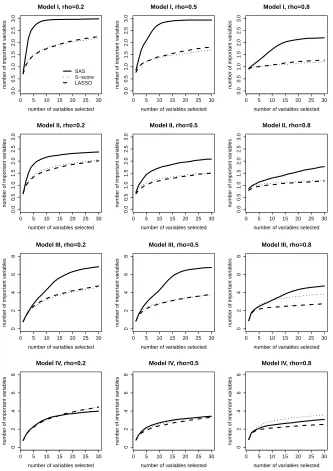
We also compare solution paths of the three methods in Figure 2.2. Here, we define a solution path as the trajectory of the number of identified important variables as the number of selected variables increases according to the selection order. For demonstration purpose, we only plot the solution paths for the first 30 selected variables. The SAS method has a natural order of selected variables. For the S-score method, we ranked the variables in descending order of the S-scores of these variables. The LASSO method has a solution path of β, which can be used to determine the order of variables entering the model. The solution path plots allow us to evaluate the ability of each method to identify important variables given that the same number of variables is selected.
Overall, the SAS method performs well on both the aspect of variable selection and the aspect of estimating optimal treatment regime. The SAS method can select most important variables at a moderate size of the selected variables. When the model is correctly specified and the correlations between covariates are not too high, the SAS method is able to identify all important variables. Moreover, the error rates of the optimal treatment regime based on the SAS method are low, and the estimated values are close to the true optimal value.
2.5.2 Multi-Stage Treatment Decisions Study
To illustrate the sequential advantage selection algorithm for multi-stage treatment decisions (MTD) study, we applied the SAS algorithm to simulated data with two-stage treatment deci-sions based on the following generative model for the final response:
Y =A1A2+A2(a+βT12X1+β21T X2) +A1(a+βT11X1) +, (2.5)
whereAk, the treatment at stagek, follows a Bernoulli distribution with parameter 0.5 fork= 1 and 2. The covariates collected at baseline,X1, include p1 = 500 variables and are denoted as X1 = (X1,1, X1,2, ..., X1,p1)
T. We generate X
1 from a multivariate normal distribution with mean zero, variance one, and correlation corr(X1,j, X1,l) = 0.2|j−l|, j 6= l. The intermediate covariates collected at the second stage are denoted by X2. For demonstration purposes, we consider a one-dimensional intermediate covariate X2 and assume that X2 = c0 +c1X1,1 +
c2A1 +c3A1X1,1+e, where the normal random error e has mean zero and variance σ22. The random error for responseY, , is normally distributed with mean zero and variance σ21.
The parameter values for the above two-stage model are chosen as follows:β12= (0,0,1,−1, 0p1−4)
T, β
21= 1, β11 = (04,1,−1,0p1−6)
intermediate covariates:c= (0,1,0,0)T, (0,0,1,0)T and (0,1,1,1)T.
Based on the generative model (2.5), it is clear that the optimal treatment regime at stage 2 isgopt2 (x1, a1, x2) = 1(a1+βT12x1+β21x2≥0). Thus, four variables (X2, A1, X1,3, X1,4) determine the optimal treatment regime at stage 2. At stage 1, the Q-function is
Q1(X1, A1) =E
|A1+β12T X1+β21X2|+
X1, A1 +A1(β11T X1) =σ2
1
√
2π exp{− µ21
2σ22}+µ1[1−Φ(−µ1/σ2)] +A1(β
T 11X1),
whereµ1=A1+βT12X1+β21[c0+c1X1,1+c2A1+c3A1X1,1]. The optimal treatment regime at stage 1 isg1opt(x1) = 1{Q1(x1,1)> Q1(x1,0)}. There are five important variables (X1,1, X1,3, X1,4,
X1,5, X1,6) for determining the optimal treatment regime at stage 1 when c= (0,1,0,0)T and (0,1,1,1)T, and four important variables (X1,3, X1,4, X1,5, X1,6) whenc= (0,0,1,0)T. Table 2.2 summarizes the optimal treatment regimes and the important variables in this simulation study. Although the optimal treatment regime and the corresponding important variables at stage 2 are explicitly defined, the optimal treatment regime at stage 1 takes a complex non-linear form. Therefore, the effects of the important variables are difficult to evaluate.
We applied the SAS algorithm to the simulated data for sample sizes n = 100, 200, and 400 over 100 replications. Simulation results are summarized in Tables 2.3 and 2.4. Table 2.3 presents results on variable selection and estimated optimal treatment regimes at both stages 1 and 2, where the same statistics as in Table 2.1 are reported (Size, TP, VR and ER). For the mean value ratio at stage 2 (VR2), we adopt random treatment regimes at stage 1 to calculate the outcome values because the optimal treatment regimes at stage 1 have not been estimated at this stage. Table 2.4 reports the proportions of each important variable being selected for all scenarios.
also increase, but 1-2 variables are missed. We will examine which variables are missed when analyzing results in Table 2.4. Based on the results for values and error rates, SAS provides good estimated optimal treatment regimes at both stages 1 and 2 when the sample size is large. We note that performances for c= (0,1,0,0)T at stage 1 are worse than the other scenarios. This indicates that the manner in which the intermediate variable depends on covariates from the last stage also affects the quality of the estimated optimal treatment regime. It is not apparent why the case with c = (0,1,0,0)T performs worse, and results in Table 2.4 partially explain this phenomenon.
Table 2.4 shows more detailed variable selection results. At stage 2, all but A1 among the four important variables can almost always be selected when the sample size is large.A1 can be selected more often forc= (0,1,0,0)T than for the other two scenarios; this may be becauseX2 depends onA1 in these cases, which partially eliminates the effects ofA1 on the final response,
Y. At stage 1, only variablesX1,5 and X1,6 can always be selected for all three scenarios when
n = 400. These two variables appear in the optimal treatment regime at stage 1 in a linear form. On the contrary, variablesX1,3,X1,4, and X1,1 that present in a non-linear form are not always selected. The probabilities of selectingX1,3 andX1,4for all three scenarios are low. This may be because these two variables do not have substantial effects on the optimal treatment regime; the high values and low error rates at stage 1 in Table 2.3 also verify this argument. The probabilities of includingX1,1differ between the first two scenarios. A possible explanation is thatX1,1 interacts with A1 inµ1 for the first scenario, which makes its sequential advantage for being selected large. This may also explain why the scenario withc= (0,1,1,1)T performs better than the scenario withc= (0,1,0,0)T in Table 2.3.
2.6
Application to STAR*D Study
We apply the proposed method to data from the STAR*D study, which was conducted to deter-mine the effectiveness of different treatments for patients with major depressive disorder (MDD) who had not been adequately benefiting from initial treatment with an antidepressant. There were 4041 participants (age 18-75) with nonpsychotic MDD enrolled in this study. Initially, these participants were treated with citalopram (CIT) up to 14 weeks. Subsequently, 3 more levels of treatments were provided for participants without a satisfactory response to CIT. At Level 2, participants were eligible for seven treatment options, which may be conceptualized as two treatment strategies: medication or psychotherapy switch, and medication or psychotherapy augmentation. Available treatments for participants to switch were: sertraline (SER), venlafax-ine (VEN), bupropion (BUP) and cognitive therapy (CT); available treatments for patients to augment were: augmenting CIT with bupropion (CIT+BUP), buspirone (CIT+BUS) or cog-nitive therapy (CIT+CT). Participants without a satisfactory response to CT were provided additional medication treatments, which is called Level 2A. All participants who did not respond satisfactorily at Level 2 or 2A were eligible for Level 3, where possible treatments were med-ication switch to mirtazapine (MIRT) or nortriptyline (NTP), and medmed-ication augmentation with either lithium (Li) or thyroid hormone (THY). Participants without satisfactory response to Level 3 were re-randomized at Level 4 to either tranylcypromine (TCP) or a combination of mirtazapine and venlafaxine (MIRT+VEN). Participants who responded satisfactorily were followed up to 1 year. See Fava et al. (2003) and Rush et al. (2004) for more detailed description of this STAR*D design.
treated with NTP and 40 were treated with MIRT at Level 3. Our goal is to identify relevant prescriptive predictors and estimate optimal dynamic treatment regimes at Levels 2 and 3 that maximize the mean response at the end of Level 3. We consider 381 covariates as possible rele-vant predictors, which are listed in Table 2.5. These covariates include participant features such as age, gender, socioeconomic status, and ethnicity; illness features such as medication history and family history of mood disorders; and care features such as clinician type. Intermediate medical conditions from Levels 1 and 2, such as degree of symptom improvement and side ef-fect burden, are also considered. For treatment regime at Level 3, all 381 covariates and the treatment at Level 2 are considered as possible predictors. For the treatment regime at Level 2, the intermediate medical conditions at Level 2 are no longer available, thus there are only 305 covariates considered for treatment decision making. We used negative 16-item Quick Inventory of Depressive Symptomatology-Clinician-Rated (QIDS-C16) at the end of Level 3 as the final response, which is a measurement of symptomatic status. Because low QIDS-C16 stands for remission, the negative QIDS-C16 was used such that larger value indicates better response.
We apply the SAS algorithm to this data set. The results are as follows. At Level 3, there are four covariates selected based on the BIC criterion: “ringing in ears” in patient rated inventory of side effects at Level 2 (EARNG-Level2), “hard to control worrying” in psychiatric diagnostic screening questionnaire at baseline (WYCRL), “feeling of worthlessness or guilt” in baseline protocol eligibility (DSMFW), and “fatigue or loss of energy” in baseline protocol eligibility (DSMLE). All four covariates are binary covariates with 1 indicating “Yes” and 0 indicating “No”. The estimated optimal treatment regime isI(−18.57 + 13.79×(EARNG-Level2)−8.46×
diagnostic screening questionnaire at baseline (EMSTP), “QIDS psychomotor agitation” in the quick inventory of depressive symptomatology - clinician at Level 1 (CAGIT), “think drink too much” in the psychiatric diagnostic screening questionnaire at baseline (DKMCH), “QIDS out-look (self)” in the quick inventory of depressive symptomatology - clinician at Level 1 (CVWSF), “IM convinced others spying” in the psychiatric diagnostic screening questionnaire at baseline (IMSPY), and “sleep at least 1-2 hours less 2 weeks” in the psychiatric diagnostic screening questionnaire at baseline (LSL2W). Among these seven covariates, TEFSH, EMSTP, DKMCH, IMSPY, and LSL2W are binary, with 1 indicating “Yes” and 0 indicating “No”; CAGIT and CVWSF are categorical covariates with 4 levels indicated by 0 to 3. The estimated optimal treatment regime is I(−5.50 + 3.91×TEFSH + 11.17 ×EMSTP + 3.76×CAGIT−4.65×
DKMCH + 4.29×CVWSF + 6.57×IMSPY−8.48LSL2W≥0), where 1 stands for treatment BUP and 0 stands for treatment SER. This optimal treatment regime assigns 39 participants to BUP and the remaining 34 participants to SER.
To further examine the estimated optimal dynamic treatment regime, we estimate the value of the estimated optimal dynamic treatment regime, that is, the mean outcome following the estimated optimal treatment regime, using the inverse probability weighted estimator proposed by Zhang et al. (2013), defined as
IPW = 1
n
n X i=1
YiI(Ai,1 =g1(Xi), Ai,2=g2(Xi))
π(Ai,1)π(Ai,2) .
Here Yi is the outcome for ith individual, Ai,1 and Ai,2 are the treatments given to the ith individual at stage 1 and stage 2, respectively,g1(Xi) and g2(Xi) are the estimated treatment regimes at stages 1 and 2, andπ(Ai,1) and π(Ai,2) are the probabilities of receiving treatment
BUP+MIRT, SER+NTP and SER+MIRT. The estimated values are shown in Table 2.6. We also report the 95% confidence intervals for the differences between values of the estimated op-timal dynamic treatment regime and the four non-dynamic treatment regimes based on 1,000 bootstrap samples. The results show that the value of the estimated optimal dynamic treat-ment regime based on the SAS algorithm is significantly larger than those of the non-dynamic treatment regimes.
2.7
Discussion
In this article, we propose a forward-stepwise variable selection method based on sequential advantage for deriving optimal treatment regimes in both single-stage and multi-stage treat-ment decision studies. Our method generalizes S-score ranking and directly targets prescriptive variables that are important for decision making. We also propose a BIC-type criterion to se-lect the number of important prescriptive variables needed for treatment decision making. The proposed method can be extended to other types of outcomes, such as categorical or censored survival data.
A two-step procedure may be used for selecting important prescriptive variables. For ex-ample, in the first step, we fit a flexible regression model of Y given A and X using some tree-based methods, such as BART or GBM. Let ˆQ(X) denote the estimated interaction effects of covariatesX and treatment indicator A. In the second step, we can consider a classification problem with responses sign{Qˆ(X)}and covariatesX, and select important covariates based on high-dimensional classification methods such as penalized logistic regression or support vector machine (SVM). Such a two-step procedure can potentially decrease the chance of missing im-portant covariates as compared to a one-step approach such as the proposed method. Although a two-step procedure looks appealing, it also has limitations. First, when pis much larger than
challeng-ing, especially when the effects are only small to moderate. Second, if the interaction effects are badly estimated in the first step, the resulting classification and selection in the second step can be erroneous.
−2 −1 0 1 2 3 −4 0 2 4 6 rho=0.2 X1 Y trt=1 trt=0
−2 −1 0 1 2 3
−4 0 2 4 6 X9 Y
−2 −1 0 1 2
−4 0 2 4 6 X10 Y
−2 −1 0 1 2 3
−2 0 2 4 rho=0.8 X1 Y trt=1 trt=0
−2 −1 0 1 2
−2 0 2 4 X9 Y
−2 −1 0 1 2
−2 0 2 4 X10 Y
Table 2.1 Simulation results of sequential advantage selection (SAS), S-score and LASSO methods in the single-stage treatment decision study.
SAS S-score LASSO
Size
ρ Size TP VR ER S6= 0 TP VR ER Size TP VR ER
Model I
0.2 6.70 2.98 99.1 5.6 765.28 1.61 84.7 27.5 21.94 1.75 79.5 32.8 (.06) (.01) (.1) (.1) (5.16) (.02) (.2) (.3) (.74) (.03) (.4) (.3) 0.5 7.56 2.91 98.5 7.4 757.18 1.31 86.7 26.6 15.04 1.37 84.2 29.4 (.08) (.01) (.1) (.2) (5.24) (.02) (.1) (.2) (.59) (.03) (.3) (.3) 0.8 8.21 1.76 94.2 17.2 738.44 1.04 94.2 18.8 11.44 1.10 93.0 20.6 (.07) (.03) (.1) (.2) (5.48) (.01) (.0) (.1) (.45) (.01) (.1) (.2) Model II
0.2 11.14 2.24 89.8 28.3 765.27 1.73 87.7 31.5 15.84 1.48 86.3 34.3 (.10) (.03) (.2) (.3) (5.23) (.02) (.2) (.3) (.68) (.03) (.2) (.3) 0.5 11.81 1.82 88.9 30.8 758.89 1.30 87.3 33.7 13.36 1.10 87.5 33.5 (.09) (.03) (.2) (.2) (5.34) (.02) (.1) (.2) (.70) (.03) (.2) (.3) 0.8 10.84 1.36 90.4 29.5 749.84 1.09 92.2 26.7 11.65 0.98 92.1 26.0 (.09) (.02) (.1) (.2) (5.38) (.01) (.1) (.2) (.48) (.02) (.2) (.3) Model III
0.2 11.73 5.13 84.2 18.3 783.39 3.38 74.7 29.1 27.09 4.03 73.4 30.9 (.13) (.12) (.7) (.5) (7.13) (.05) (.4) (.3) (1.15) (.10) (.4) (.3) 0.5 10.41 4.67 87.0 18.6 776.15 2.88 78.3 28.1 25.05 3.24 77.6 29.3 (.11) (.10) (.5) (.4) (7.38) (.04) (.3) (.2) (1.17) (.08) (.3) (.3) 0.8 7.74 3.01 90.0 19.6 760.68 2.93 90.9 20.3 17.37 2.49 88.5 22.2 (.10) (.05) (.1) (.2) (7.62) (.03) (.1) (.2) (.67) (.04) (.2) (.2) Model IV
Table 2.2 Optimal Treatment Regimes and Corresponding Important Variables in Multi-Stage Simula-tion Study
Optimal Treatment Regime Important Variables Stage 2 1(a1+β12Tx1+β21x2 ≥0) (X2, A1, X1,3, X1,4)
Stage 1 1{Q1(x1,1)> Q1(x1,0)}
c= (0,1,0,0)T
(X1,1, X1,3, X1,4, X1,5, X1,6) and (0,1,1,1)T
c= (0,0,1,0)T (X1,3, X1,4, X1,5, X1,6)
Table 2.3 Simulation Results of SAS-MTD method for Two-Stage Treatment Decisions Study.
Stage 2 Stage 1
n Size TP VR2 ER Size TP VR1 ER
c= (0,1,1,1)T
100 5.22 (.46) 2.08 (.09) 85.3 17.8 6.29 (.36) 0.70 (.07) 73.1 26.9 200 4.08 (.11) 3.25 (.06) 94.3 8.8 5.43 (.25) 2.34 (.10) 93.4 14.5 400 4.02 (.06) 3.75 (.04) 97.5 4.4 3.61 (.11) 3.14 (.04) 98.2 8.5 c= (0,1,0,0)T
100 6.70 (.28) 1.80 (.11) 67.7 24.9 8.88 (.35) 0.45 (.07) 49.1 39.8 200 6.38 (.21) 3.48 (.06) 89.7 13.5 11.80 (.27) 1.78 (.08) 78.2 26.6 400 5.82 (.19) 3.88 (.03) 96.1 7.8 13.01 (.36) 2.41 (.07) 92.7 16.6 c= (0,0,1,0)T
0 5 10 15 20 25 30 0.0 0.5 1.0 1.5 2.0 2.5 3.0
Model I, rho=0.2
number of variables selected
n
umber of impor
tant v ar iab les SAS S−score LASSO
0 5 10 15 20 25 30
0.0 0.5 1.0 1.5 2.0 2.5 3.0
Model I, rho=0.5
number of variables selected
n
umber of impor
tant v
ar
iab
les
0 5 10 15 20 25 30
0.0 0.5 1.0 1.5 2.0 2.5 3.0
Model I, rho=0.8
number of variables selected
n
umber of impor
tant v
ar
iab
les
0 5 10 15 20 25 30
0.0 0.5 1.0 1.5 2.0 2.5 3.0
Model II, rho=0.2
number of variables selected
n
umber of impor
tant v
ar
iab
les
0 5 10 15 20 25 30
0.0 0.5 1.0 1.5 2.0 2.5 3.0
Model II, rho=0.5
number of variables selected
n
umber of impor
tant v
ar
iab
les
0 5 10 15 20 25 30
0.0 0.5 1.0 1.5 2.0 2.5 3.0
Model II, rho=0.8
number of variables selected
n
umber of impor
tant v
ar
iab
les
0 5 10 15 20 25 30
0
2
4
6
8
Model III, rho=0.2
number of variables selected
n
umber of impor
tant v
ar
iab
les
0 5 10 15 20 25 30
0
2
4
6
8
Model III, rho=0.5
number of variables selected
n
umber of impor
tant v
ar
iab
les
0 5 10 15 20 25 30
0
2
4
6
8
Model III, rho=0.8
number of variables selected
n
umber of impor
tant v
ar
iab
les
0 5 10 15 20 25 30
0
2
4
6
8
Model IV, rho=0.2
number of variables selected
n
umber of impor
tant v
ar
iab
les
0 5 10 15 20 25 30
0
2
4
6
8
Model IV, rho=0.5
number of variables selected
n
umber of impor
tant v
ar
iab
les
0 5 10 15 20 25 30
0
2
4
6
8
Model IV, rho=0.8
number of variables selected
n
umber of impor
tant v
ar
iab
les
Table 2.4 Proportion of Each Important Variable Being Selected at Stage 2 and Stage 1.
Stage 2 Stage 1
n X1,3 X1,4 X2 A1 X1,3 X1,4 X1,5 X1,6 X1,1
1 -1 1 1 * * 1 -1
*/-c= (0,1,1,1)T
100 0.58 0.49 0.85 0.16 0.01 0.01 0.13 0.08 0.47 200 0.95 0.96 0.97 0.37 0.02 0.03 0.72 0.71 0.86 400 1.00 1.00 1.00 0.75 0.07 0.07 1.00 1.00 1.00 c= (0,1,0,0)T
100 0.59 0.51 0.55 0.15 0.01 0.00 0.24 0.16 0.04 200 0.99 1.00 0.92 0.57 0.03 0.04 0.82 0.84 0.05 400 1.00 1.00 0.98 0.90 0.17 0.07 1.00 1.00 0.17 c= (0,0,1,0)T
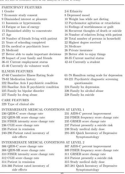
Table 2.5 List of covariates used in the analysis of STAR*D study.
PARTICIPANT FEATURES
1 Gender 2-6 Ethnicity
7 Economic study consent 8 Depressed mood
9 Diminished interest or pleasure 10 Weight loss while not dieting
11 Insomnia or hypersomnia 12 Psychomotor agitation or retardation 13 Fatigue or loss of energy 14 Feelings of worthlessness or guilt 15 Diminished ability to concentrate 16 Recurrent thoughts of death or suicide
17 Age 18 Number of relatives living with patient
19 Number of friends living with patient 20 Total number of persons in household 21 Years of schooling completed 22 Highest degree received
23 On medical or psychiatric leave 24 Medicare
25 Medicaid 26 Private insurance
27 Better able to make important decisions 28 Better able to enjoy things 29 Impact of your family and friends 30-35 Current marital status 36-41 Current employment status 42-44 Currently a student 45-46 Currently do volunteer work
ILLNESS FEATURES
47-60 Cumulative Illness Rating Scale 61-78 Hamilton rating scale for depression 79-82 Medication history 83-221 Psychiatric diagnostic screening 222 Baseline Axis I psychiatric condition questionnaire
223 Baseline Axis II psychiatric condition 224 Family hx depression 225 Family hx bipolar disorder 226 Family hx alcohol abuse 227 Family hx drug abuse 228 Family hx suicide CARE FEATURES
229 Type of clinical site
INTERMEDIATE MEDICAL CONDITIONS AT LEVEL 1
230 QIDS-C score change rate 231 AIDS-C percent improvement 232 QIDS-SR score change rate 233 FISER frequency score change rate 234 FISER intensity score change rate 235 GRSEB score change rate
236 CGII score change rate 237 Patient presently a suicide risk 238 Patient in remission 239 Study medical daily dose
240-290 Patient rated inventory of 291-305 Quick Inventory of Depressive
side effects Symptomatology
INTERMEDIATE MEDICAL CONDITIONS AT LEVEL 2
306 QIDS-C score change rate 307 AIDS-C percent improvement 308 QIDS-SR score change rate 309 FISER frequency score change rate 310 FISER intensity score change rate 311 GRSEB score change rate
Table 2.6 Estimated Values of Different Treatment Regimes and Confidence Intervals for the Differ-ences of Values.
Treatment Regime Estimated Value Diff 95% CI on Diff optimal regime from SAS-MTD -5.26
BUP + NTP -13.27 8.01 [2.83,13.64]
BUP + MIRT -11.71 6.45 [1.83,11.02]
SER + NTP -13.15 7.89 [1.94,13.72]
Chapter 3
PENALIZED A-LEARNING FOR
OPTIMAL TREATMENT
DECISIONS WITH
NP-DIMENSIONALITY
3.1
Introduction
including Q-learning (Watkins and Dayan, 1992; Chakraborty et al., 2010) and A-learning (Robins et al., 2000; Murphy, 2003). Both Q-learning and A-learning rely on a backward in-duction algorithm to find the optimal dynamic treatment regime, however, Q-learning models the conditional mean of the outcome given predictors and treatment whileA-learning directly models the contrast function that is sufficient for treatment decision. In particular, A-learning has the so-called double robustness property, i.e. when either the baseline mean function or the propensity score model is correctly specified, the resulting A-learning estimating equation for the contrast function is consistent.
The rapid advances and breakthrough in technology and communication systems make it possible to gather an extraordinary large number of prognostic factors for each individual, such as patient’s genetic information, demographic characteristics, medical history and clinical measurements over time. With such data gathered at hand, it is of significant importance to organize and integrate information that is relevant to make optimal individualized treatment decisions, which makes variable selection as an emerging need for implementing personalized medicine with big data. In addition, variable selection is an essential tool in making inference for problems in which the number of covariates is comparable or much larger than the sample size. There have been extensive developments of penalized methods for variable selection in prediction, for example, LASSO (Tibshirani, 1996), SCAD (Fan and Li, 2001) and Dantzig selector (Cand`es and Tao, 2007), to name a few. In contrast to most penalized regression methods, which adds a penalty term to an objective function, the Dantzig selector focused directly on estimating equations.
However, the associated variable selection properties, such as selection consistency, convergence rate and oracle distribution, are not studied. Lu et al. (2013) introduced a new penalized least squares regression framework, which is robust against the misspecification of the conditional mean function. However, they only studied the case when the number of covariates is fixed and the propensity score model is known as in randomized clinical trials.
In this chapter, we propose a penalized A-learning method for deriving the optimal dynamic treatment regime when the number of covariates is of the non-polynomial (NP) order of the sample size. To preserve the double robustness property of the A-learning method, we adopt the Dantzig selector Cand`es and Tao (2007) which directly penalizes the A-leaning estimating equations.
The remainder of this chapter is organized as follows. We introduce our proposed penalized A-learning method in Section 3.2. Some implementation issues are addressed in Section 3.3, followed by simulation results in Section 3.4. We apply our method to a data from the STAR*D study in Section 3.5.
3.2
Penalized A-Learning
For simplicity of presentation, we only consider a two-stage study where binary treatment decisions are made at time points t1 and t2. The data of a subject can be summarized as
O = (S(1), A(1), S(2), A(2), Y), (3.1)
treatment regime to maximize the mean outcome. Throughout this chapter, we make the stable unit treatment value assumption and sequential randomization assumption (Murphy, 2003) as standard for studying dynamic treatment regimes.
The observed data of n subjects can be summarized as
Oi = (Si(1), A(1)i , Si(2), A(2)i , Yi), i= 1, . . . , n,
which are assumed to be independently and identically distributed copies ofO. We assume the following semiparametric regression model forY:
Yi=h(2)(Xi) +Ai(2)(XiTβ2) +ei, (3.2)
where Xi = ((Si(1))T, A (1) i ,(S
(2)
i )T)T is the vector of covariates for the ith patient, whose first element is 1, h(2)(·) is an unspecified baseline mean function and ei is an independent error with mean 0. The design matrix is denoted asX = (X1, . . . , Xn)T.
Define
Vi(2)= max A(2)i
E(Yi|Si(1), A (1) i , S
(2) i , A
(2)
i ) =h(2)(Xi) +XiTβ2I(XiTβ2>0),
whereI(·) stands for the indicator function. At the first stage, we consider the following model forV(2):
Vi(2)=h(1)(Si(1)) +A(1)i C(Si(1)) +i, (3.3)
It can be shown that the optimal dynamic treatment regime is given by dopt = (dopt1 , dopt2 ), wheredopt1 and dopt2 take the form
dopt1 (Si) =I(C(Si)>0) and dopt2 (Xi) =I(XiTβ2 >0). (3.4)
To estimatedopt1 anddopt2 , we posit the following models forC(·),h(1)(·),h(2)(·),π(1)(·), and
π(2)(·):
π(1)(s, α1) = exp(sTα1)/{1 + exp(sTα1)}, (3.5)
π(2)(x, α2) = exp(xTα2)/{1 + exp(xTα2)}, (3.6)
h(1)(s) =sTθ1, h(2)(x) =xTθ2, C(s) =sTβ1. (3.7)
where the first elements of x ands are 1,
π(1)(s) = Pr(A(1)i = 1|Si =s) and π(2)(x) = Pr(A(2)i = 1|Xi =x).
Models in (3.5)-(3.7) can be misspecified, however, we require that either h(j) or π(j) is correct for j = 1,2. As in A-learning, we use backward induction to estimate the optimal dynamic treatment regime. At the second decision point, we first estimate the parameters in the posited propensity score and baseline mean models using penalized regressions. Specifically, define
ˆ
α2 = arg min α2∈Rp
1
n
n X i=1
[log{1 + exp(XiTα2)} −A(2)i X T i α2] +
p X j=1
and
ˆ
θ2= arg min θ2∈Rp
1
n
n X i=1
(1−A(2)i )(Yi−XiTθ2)2+ p X j=1
ρ(2)2 (|θj2|, λ(2)2n),
where α2 = (α12,· · ·, α p
2)T and θ2 = (θ21,· · · , θ p
2)T, and ρ (2) 1 and ρ
(2)
2 belong to the class of concave penalty functions (Lv and Fan, 2009).
Next, we estimate β2 in (3.2) using the Dantzig selector based on A-learning estimating function (Murphy, 2003), defined by
ˆ
β2= arg min β2∈Λ(2)
||β2||1, (3.8)
where
Λ(2)=
β2 ∈Rp :||1
nX
Tdiag(A(2)−πˆ(2)){Y −Xθˆ
2−A(2)◦(Xβ2)}||∞≤λ(2)3n
,
A(2)= (A(2)1 , . . . , An(2))T and πˆ(2)= (π(X1,αˆ2), . . . , π(Xn,αˆ2))T.
To estimate the regime at the first decision point, we estimate Vi(2) using the advantage function (Murphy, 2003) by
ˆ
Vi=Yi+XiTβˆ2{I(XiTβˆ2 >0)−A(2)i }. (3.9)
Similarly, define
ˆ
α1 = arg min α1∈Rq
1
n
n X
i=1
[log{1 + exp(STi α1)} −A(1)i SiTα1] + q X j=1
and
ˆ
θ1= arg min θ1∈Rq
1
n
n X i=1
(1−A(1)i )( ˆVi−SiTθ1)2+ q X j=1
ρ(1)2 (|θj1|, λ(1)2n),
where α1 = (α11,· · ·, α q
1)T and θ1 = (θ11,· · ·, θ q
1)T, andρ (1) 1 and ρ
(1)
2 are concave penalty func-tions. Then, we estimate β1 in (3.3) by
ˆ
β1= arg min β1∈Λ(1)
||β1||1, (3.10)
where
Λ(1)=
β1 ∈Rq:||1
nS
Tdiag(A(1)−πˆ(1)){Y −Sθˆ
1−A(1)◦(Sβ1)}||∞≤λ(1)3n
,
A(1) = (A(1)1 , . . . , An(1))T and πˆ(1)= (π(S1,αˆ1), . . . , π(Sn,αˆ1))T.
The estimated optimal dynamic treatment regime is given by
ˆ
d1(Si) =I( ˆβ1TSi>0) and dˆ2(Xi) =I( ˆβ2TXi>0). (3.11)
3.3
Some Implementation Issues
When the tuning parameters in optimization problems (3.8) and (3.10) are fixed, the Dantzig selector can be solved by a standard linear programming algorithm. One issue for implementing Dantzig selector is the choice of the tuning parameters. We use a BIC criterion for selecting tuning parameters. For Dantzig selector (3.8),λ(2)3n is chosen as the minimizer of
where RSS(λ) = Pn i=1
h
{A(2)i −π(2)(Xi,αˆ2)}(Y (2)
i −XiTθˆ2−A (2) i XiTβˆ2)
i2
, and d(λ) is the number of nonzero components in ˆβ2. A similar BIC criterion was proposed by Chen and Chen (2008). We use a similar criterion for choosingλ(1)3n.
It was observed that the Dantzig estimators may underestimate the true values of param-eters due to the shrinkage estimation(Cand`es and Tao, 2007). Therefore, we use a two-step procedure for practical implementation, which is referred as Gauss-Dantzig selector in Cand`es and Tao (2007). Specifically, in the first step, we apply the proposed penalized A-learning to select important variables for making an optimal decision, i.e. those variables with non-zero es-timated coefficients. Then, in the second step, their corresponding coefficients are re-calculated by solving the unpenalized A-learning estimating equations with important variables only.
3.4
Simulation Studies
3.4.1 Settings
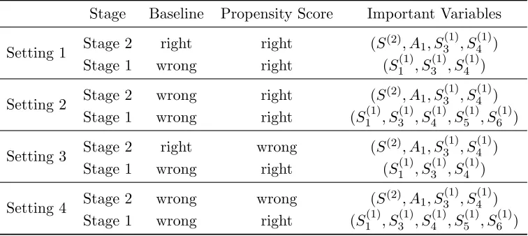
To evaluate the numerical performance of the proposed penalized A-learning method, we con-sider simulation studies with two treatment decision points, based on the following model:
Y =A1A2+A2(β12TS(1)+β21S(2)) +A1(β11T S(1)) +, (3.13)
where Aj, j = 1,2, is the treatment given at the jth stage, S(j), j = 1,2, denote the covariate information collected before thejth treatment is given, andY is the final response of interest. Random error follows a normal distribution with mean 0 and variance σ12. Treatment Aj takes two values: 0 and 1, and two models are considered for the propensity scores: constant model, P(Aj = 1) = 0.5, and probit models. Here, covariates S(1) = (S1(1), ..., S
(1)