1602
A Comparative Analysis of Different Data mining
algorithm for Credit risk modeling
Jismy Joseph1, Dr.G. Kesavaraj2
PhD Research Scholar1, Professor and head2
Department of Computer Science, Vivekanandha College of Arts and
Science for Women (Autonomous), Elayampalayam, Thiruchengode, Tamil Nadu, India Email: [email protected], [email protected]
Abstract- Analysis of credit risk is a data mining problem deserving serious consideration in financial risk governance. The abundance of data generated daily in banks and other financial sectors poses a challenge in the realm of data mining. This paper compares the accuracy and efficiency of twelve data mining algorithms –Naïve Bayes, Bayes Net, Simple Logistic, SMO, Decision Table, OneR, ZeroR, J48, Random Forest, IBk, KStar and REPTree by applying them to three credit data sets. Experiment results show that Random Forest algorithms produced the best classification accuracy, On the contrary, the ZeroR algorithm produced low accuracy.
Index Terms
- Data Mining, Classification, Machine learning, Weka.
1. INTRODUCTION
The concept of banking in recent times has undergone vast changes that have been accompanied by emergence of new risks and worsening of existing ones. In such a scenario, credit risk analysis becomes a challenging and emerging field in data mining. A highly desired usage of economic capital can be achieved by a thorough evaluation of credit risk. There are different types of credit risks. It can be credit default risk, country risk or a concentration risk [1]. Data mining techniques can extract hidden information from huge data set, this knowledge will help the bankers to analyze the credit risk.
Data mining is also known as KDD (Knowledge Discovery in Databases), is used to retrieve potentially useful information from huge amount of data. In many emerging fields like retail, bioinformatics education and financial enterprises are using data mining algorithms for knowledge recovery. The main stages of KDD are data selection, data preprocessing, data projection, data mining, and knowledge recovery. In this paper I have used the tool Weka for analyzing different data mining algorithms. Weka is an open source data mining software developed by University of Waikato, New Zealand and it contains different machine learning algorithms.
2. LITERATURE REVIEW
To predict credit risk already many research work are done. In the paper ‘Comparative Analysis of Data Mining Classification Algorithms in Type-2 Diabetes Prediction Data Using WEKA Approach’ [2] Kawsar Ahmed, Tasnuba Jesmin compared speed and accuracies of different data mining classifications and
then ranked the best 5 algorithms. They used type-2 diabetes disease dataset.
In [3] Aman Kumar Sharma , Suruchi Sahni in their paper they conducted experiment in the WEKA environment by using four algorithms namely ID3, J48, Simple CART and Alternating Decision Tree on the spam email dataset and later the four algorithms were compared in terms of classification accuracy. According to their simulation results, the J48 classifier outperforms the ID3, CART and ADTree in terms of classification accuracy.
In [4] Satish Kumar David, Amr T.M. Saeb, Khalid Al Rubeaan, 2013 they compared algorithms based on their accuracy, learning time and error rate and they observed that there is a direct relationship between execution time in building the tree model and the volume of data records, while there is also an indirect relationship between execution time in building the model and the attribute size of the data sets. They concluded that Bayesian algorithms have better classification accuracy over and above compared algorithms.
In [5] Shrey Bavisi, Jash Mehta, Lynette Lopes concluded that The Naïve Bayes model is simple, elegant and extremely robust, making it way more appealing. On the other hand it is an easily understood and easily implemented classification technique. C4.5 algorithm is also used in classification problems where it is used to build decision trees. C4.5 deals with both numeric attributes as well as missing values, making it suitable for dealing with real life problems.
1603 data mining algorithms - logistic regression (LR),
decision tree (C4.5), support vector machine (SVM) and neural networks (NN). They used two credit data sets and the result shows that the LR and SVM algorithms produced the best classification accuracy, and the SVM shows the higher robustness and generalization ability compared to the other algorithms. On the contrary, the neural networks algorithm performed poorly on the two credit data sets in their experiments.
3. DATA SETS AND CLASSIFIERS
I have used three set of credit data from UCI repository for comparing twelve algorithms to find credit risk. The first data set is an Australian credit data set. This data set consists of 15 attributes and 690 instances. The second set is a Japanese credit data which has 16 attributes and 690 instances. The third one is a German credit Data set with 21 attributes and 1000 instances. In this comparative study 12 classification algorithms are used. In Weka these classifiers are categorized into different groups such a trees, rules, bays, function and lazy. The classification algorithms are:
3.1. IBK
Knn is an instance based and non parametric classification algorithm. It uses k closest instances to predict target class. These nearest instances are calculated by using distance measures. Euclidean, Manhattan, Minkowski and Hamming are commonly used different distance measures. For continuous variables Euclidean, Manhattan, Minkowski are valid but for categorical variables Hamming distance is used. In Knn, the classification of a case is based on the highest number of votes of its neighbors and the case is assigned to the most common class, its K nearest neighbors.
3.2. SMO
SMO is one method to solve SVM problems. Support Vector machine is a supervised classification algorithm, also used for regression analysis. SVM can perform linear and non linear classification. In this algorithm, each data items are plotted as a point in n-dimensional space (where n is number of features you have) with the value of each feature being the value of a particular coordinate.
3.3. Bayes Net
Bayes Net, also called Bayesian Networks are structured graphic models of probabilistic relationship between random variables. In this model the node of the graph denotes the random variables and the edges represent the conditional dependencies between the
variables. In this method the models are made from probability distribution and it uses the probability law for prediction.
3.4. Simple Logistic
Simple Logistic classifier is used to build linear logistic regression model. If I have a nominal variable and a measurement variable then I can use simple logistic model to predict the probability of whether change in the measurement variable can causes change in the nominal variable. Here the nominal variable is dependent and measurement variable is independent.
3.5. Naïve Bayes
Naïve Bayes is a powerful and straightforward algorithm for classification. This approach can work on data set that has millions of records [7]. It is a supervised learning method based on conditional probability and also using independent assumption. The probability of an event can be calculated by using the conditional probability. The following formula is used for calculating the conditional probability. P (H/E) = (P (E/H)*P (H))/P (E).
3.6. Random Forest
Random Forest is a supervised machine learning algorithm used for classification and regression. These classifiers handle the missing values and can model the categorical values It creates many decision trees and merges them together to form an accurate prediction. In the method the parameters are used to increase the predictive power and speed of the model.
3.7. OneR
OneR is a fast, accurate and Reproducible algorithm can handle only categorical data. By using frequency table it creates a rule for a predictor and select the rule has lowest error as its rule.
3.8. REPTree
REP Tree is a regression based classifier, it generate multiple trees in different iteration and select best one from these and is considered as the representative one.
3.9. Kstar
1604
4. RESULT AND OBSERVATION
The algorithms are executed by using the ‘Explorer’ option of the Weka tool. Firstly, the text data set is converted into ARFF format and submitted to Weka then data preprocessing is performed to create quality data. After that data classification is done for finding the data models.
4.1. Classification of data set 1
The first data set is an Australian credit data set with 15 attributes and 690 instances. The algorithm Random forest has highest accurate rate 87%. 8 out of
12 algorithms got accuracy more than 80%. The algorithm ZeroR got lowest accurate rate 56%. 86.9% of the instances are correctly classified by random Forest. Table 1 shows that RandomForest, Simple logistic, Decision table and ONeR performed better than the remaining algorithms. The SMO and simple logistic took more time (0.36 sec, 0.34 sec) for classification whereas the remaining algorithms took almost less than 0.3 second. The Kappa statistic of Simple Logistic, SMO, Decision Table, Random Forest and OneR are almost same (0.7)
Table 1:- Comparison of different classifiers uses Australian credit data set with 15 attributes and 690 instances
Australian credit data set
Algorithms )
Correctly Classified Instances (%)
Incorrectl y
Classified Instances (%)
Kappa Statisti c
Time taken (In sec)
Mean
Absolute Error
Root Mean Square d Error
Relative
Absolute Error (%)
Root relative Squared Error (%) Naïve Bayes 77.2464 22.7536 0.5244 0.02 0.2255 0.439 45.6478 88.3326 Bayes Net 84.9275 15.0725 0.6929 0.04 0.1713 0.3414 34.6709 68.6899 Simple
Logistic
85.942 14.058 0.7177 0.34 0.2058 0.3187 41.6662 64.128
SMO 85.5072 14.4928 0.7116 0.36 0.1449 0.3807 29.3397 76.6032
Decision Table
85.7971 14.2029 0.7134 0.19 0.2513 0.3423 50.8749 68.8834
OneR 85.5072 14.4928 0.7116 0.02 0.1449 0.3807 29.3397 76.6032
ZeroR 55.5072 44.4928 0 0 0.494 0.497 100 100
J48 85.2174 14.7826 0.6997 0.06 0.1822 0.3517 36.8881 70.7605
Random Forest
86.9565 13.0435 0.7368 0.29 0.202 0.3093 40.8967 62.2472
IBk 80 20 0.5956 0 0.201 0.4465 40.6838 89.8444
KStar 79.1304 20.8696 0.568 0.01 0.2215 0.4066 44.8386 81.8124
1605 Figure 1- Comparison -Accuracy, Sensitivity & Specificity
Table2: Comparison of accuracy, sensitivity & specificity in Australian credit data set
.
Australian credit Data set
Algorithms TP FN FP TN
Sensitivity= TP / (TP+FN)
Specificity = TN / (TN+FP)
Accuracy = (TP+TN)/ (TP+FN+FP+TN)
Naïve Bayes 353 30 127 180 0.92 0.59 0.77
Bayes Net 341 42 62 245 0.89 0.80 0.85
Simple
Logistic 322 61 36 271 0.84 0.88 0.86
SMO 306 77 23 284 0.80 0.93 0.86
Decision Table 329 54 44 263 0.86 0.86 0.86
OneR 306 77 23 284 0.80 0.93 0.86
ZeroR 383 0 307 0 1.00 0.00 0.56
J48 337 46 56 251 0.88 0.82 0.85
Random Forest 333 50 40 267 0.87 0.87 0.87
IBk 312 71 67 240 0.81 0.78 0.80
KStar 345 38 106 201 0.90 0.65 0.79
REPTree 316 67 38 267 0.83 0.88 0.85
4.2.Classification of data set 2
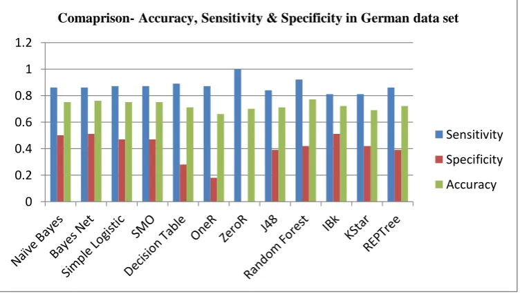
The second data set is a German credit Data set with 21 attributes and 1000 instances. When the size of the data set is increased, the accuracy of all algorithms are reduced. However the classifier random Forest got highest accuracy. All the classifier expects Oner, ZeroR and Kstar produced more than 70% accuracy.
Simple Logistic took highest time (1.61sec) for making models. Expect simple logistic and SMO all other algorithms used less than 1 sec to make the models. 76.8 % of the instances are correctly classified by Random forest. Simple Logistic and Bays net classified instances correctly by more than 75%. 0
0.1 0.2 0.3 0.4 0.5 0.6 0.7 0.8 0.91
Comparison -Accuracy, sensitivity & specificity
1606 Table 3:- Comparison of different classifiers uses German credit data set with 21 attributes and 1000 instances.
Figure 2- Comparison -Accuracy, Sensitivity & Specificity.
0 0.2 0.4 0.6 0.8 1 1.2
Comaprison- Accuracy, Sensitivity & Specificity in German data set
Sensitivity Specificity Accuracy German credit Data set
Algorithms )
Correctl y Classifie d Instance s (%)
Incorrectl y
Classified Instances (%)
Kappa Statisti c
Time taken (In sec)
Mean
Absolute Error
Root Mean Square d Error
Relative
Absolute Error (%)
Root relative Squared Error (%)
Naïve Bayes 75.4 24.6 0.3813 0.01 0.2937 0.4201 69.9042 91.67 Bayes Net 75.5 24.5 0.3893 0.04 0.3102 0.4187 73.8182 91.3674 Simple
Logistic
75.9 24.1 0.392 1.61 0.3127 0.4037 74.4267 88.084
SMO 75.2 24.8 0.3673 1.36 0.248 0.498 59.0227 108.671 Decision Table 71 29 0.2033 0.33 0.3677 0.4321 87.505 94.2815 OneR 66.1 33.9 0.0552 0.02 0.339 0.5822 80.6802 127.054 ZeroR 70 30
0
0 0.4202 0.4583 100 100
J48 70.7 29.3 0.2503 0.1 0.3459 0.4793 82.3125 104.588
Random Forest
76.8 23.2 0.379 0.34 0.3362 0.4028 80.0091 87.8987
1607 Table4: Comparison of accuracy, sensitivity & specificity in German credit data set.
German credit data set
Algorithms TP FN FP TN
Sensitivity= TP / (TP+FN)
Specificity = TN / (TN+FP)
Accuracy = (TP+TN)/ (TP+FN+FP+TN)
Naïve
Bayes 605 95 151 149 0.86 0.50 0.75
Bayes Net 601 99 146 154 0.86 0.51 0.76
Simple
Logistic 611 89 159 141 0.87 0.47 0.75
SMO 611 89 159 141 0.87 0.47 0.75
Decision
Table 625 75 215 85 0.89 0.28 0.71
OneR 607 93 246 54 0.87 0.18 0.66
ZeroR 700 0 300 0 1.00 0.00 0.70
J48 590 110 183 117 0.84 0.39 0.71
Random
Forest 642 58 174 126 0.92 0.42 0.77
IBk 567 133 147 153 0.81 0.51 0.72
KStar 569 131 175 125 0.81 0.42 0.69
REPTree 601 99 183
117
0.86
0.39
0.72
4.3. Classification of data set 3
The third data set is uses Japanese credit Data with 16 attributes and 690 instances. In this data set, the number of attributes and instances are also less compared to second data set, therefore the accuracy of all algorithms are high in this case. The highest
accuracy is 87%, produced by Random forest. The accuracy of Bayes Net, Simple Logistic, SMO, OneR, J48 and REPTree are also greater than or equal to 85%. ZeroR has the lowest accuracy rate 56%. 86.7% of the instances are correctly classified by random Forest. All the algorithms took less than 1 sec.
Figure 3- Comparison -Accuracy, Sensitivity & Specificity
0 0.2 0.4 0.6 0.8 1 1.2
Comparison- accuracy, Senitivity & specificity in Japanese data set
1608 Table 5: Comparison of different classifiers using Japanese credit data set with 16 attributes and 690 instances.
Table6: Comparison of accuracy, sensitivity & specificity in Japanese credit data set Japanese credit Data set
Algorith ms
Correctl y Classifie d Instance s (%)
Incorrec tly Classifie d Instance s (%)
Kappa Statistic
Time taken (In second s)
Mean
Absolut e Error
Root Mean Square d Error
Relative
Absolute Error (%)
Root relative Squared Error (%)
Naïve Bayes
77.6812 22.3188 0.534 0.02 0.2228 0.2228 45.0957 87.6395
Bayes Net 86.2319 13.7681 0.7186 0.04 0.163 0.3335 32.9964 67.1144 Simple
Logistic
84.9275 15.0725 0.698 0.58 0.2127 0.3248 43.0642 65.3608
SMO 84.9275 15.0725 0.7003 0.62 0.1507 0.3882 30.5133 78.1202 Decision
Table
83.4783 16.5217 0.6672 0.14 0.2255 0.335 45.6465 67.4073
OneR 85.5072 14.4928 0.7116 0.02 0.1449 0.3807 29.3397 76.6032
ZeroR 55.5072 44.4928 0
0.01 0.494 0.497 100 100
J48 86.087 13.913 0.718 0.04 0.1924 0.3313 38.9417 66.6637 Random
Forest
86.6667 13.3333 0.7295 0.25 0.2294 0.3216 46.4412 64.706
IBk 81.1594 18.8406 0.6178 0 0.1894 0.4334 38.3442 87.2014 KStar 78.9855 21.0145 0.5666 0.01 0.2259 0.4117 45.734 82.8457 REPTree 85.6522 14.3478 0.712 0.04 0.2145 0.3358 43.4255 67.5631
Japanese Credit data set
Algorithms TP FN FP TN
Sensitivity= TP / (TP+FN)
Specificity = TN / (TN+FP)
Accuracy = (TP+TN)/ (TP+FN+FP+TN)
Naïve Bayes 183 124 30 353 0.60 0.92 0.78
Bayes Net 245 62 33 350 0.80 0.91 0.86
Simple
Logistic 271 36 68 315 0.88 0.82 0.85
SMO 283 24 80 303 0.92 0.79 0.85
Decision
Table 258 49 65 318 0.84 0.83 0.83
OneR 284 23 77 306 0.93 0.80 0.86
ZeroR 0 307 0 383 0.00 1.00 0.56
J48 257 50 46 337 0.84 0.88 0.86
Random
Forest 258 49 43 340 0.84 0.89 0.87
IBk 239 68 62 321 0.78 0.84 0.81
KStar 206 101 44 339 0.67 0.89 0.79
1609
5. CONCLUSION
This paper focused on trying to find the best algorithm for credit risk modeling. This study observed that Random Forest algorithm obtained highest acuracy in all the data sets. It produced 85% of accuracy in Australian data set , 77% in german data set and 86% in japanese data set. However developing a new algorithm for credit risk analysis is necessary to increase the accuracy.
REFERENCES
[1] Credit and Financial risk analyis. (2016). Retrieved from http://www.credfinrisk.com: http://www.credfinrisk.com/basics.html.
[2] Aman Kumar Sharma , Suruchi Sahni . (2011). A Comparative Study of Classification Algorithms.
International Journal on Computer Science and Engineering (IJCSE), 1890-1895.
[3] Hong Yu, Xiaolei Huang, Xiaorong Hu, Hengwen Cai. (2010). A Comparative Study on Data Mining Algorithms for Individual Credit Risk Evaluation. IEEE Xplore.
[4] Kawsar Ahmed, Tasnuba Jesmin. (2014). Comparative Analysis of Data Mining Classification Algorithms in Type-2 Diabetes
Prediction Data Using WEKA Approach. IJSE, vol-7,155.
[5] Satish Kumar David, Amr T.M. Saeb, Khalid Al Rubeaan. (2013). Comparative Analysis of Data Mining Tools and Classification Techniques using WEKA in Medical Bioinformatics. IISTE. [6] Saxena, R. (2017, February 7).
http://dataaspirant.com/2017/02/06/naive-bayes-classifier-machine-learning. Retrieved May Tuesday, 2018, from http://dataaspirant.com: http://dataaspirant.com/2017/02/06/naive-bayes-classifier-machine-learning/
[7] Shrey Bavisi, Jash Mehta, Lynette Lopes. (2014). A Comparative Study of Different Data Mining Algorithms. International Journal of Current Engineering and Technology , 3248-3252. [8] Vijayarani, S., & Muthulakshmi, M. (2013).