Classifying chart cells for quadratic complexity context-free inference
Brian Roark and Kristy Hollingshead Center for Spoken Language Understanding
Oregon Health & Science University, Beaverton, Oregon, 97006 USA
{roark,hollingk}@cslu.ogi.edu
Abstract
In this paper, we consider classifying word positions by whether or not they can either start or end multi-word constituents. This provides a mechanism for “closing” chart cells during context-free inference, which is demonstrated to improve efficiency and accuracy when used to constrain the well-known Charniak parser. Additionally, we present a method for “closing” a sufficient number of chart cells to ensure quadratic worst-case complexity of context-free in-ference. Empirical results show that this
O(n2)bound can be achieved without
im-pacting parsing accuracy.
1 Introduction
While there have been great advances in the statis-tical modeling of hierarchical syntactic structure in the past 15 years, exact inference with such mod-els remains very costly, so that most rich syntac-tic modeling approaches involve heavy pruning, pipelining or both. Pipeline systems make use of simpler models with more efficient inference to re-duce the search space of the full model. For ex-ample, the well-known Ratnaparkhi (1999) parser used a POS-tagger and a finite-state NP chunker as initial stages of a multi-stage Maximum Entropy parser. The Charniak (2000) parser uses a simple PCFG to prune the chart for a richer model; and Charniak and Johnson (2005) added a discrimina-tively trained reranker to the end of that pipeline.
Recent results making use of finite-state chun-kers early in a syntactic parsing pipeline have shown both an efficiency (Glaysher and Moldovan, 2006) and an accuracy (Hollingshead and Roark, 2007) benefit to the use of such constraints in a parsing system. Glaysher and Moldovan (2006) demonstrated an efficiency gain by explicitly dis-allowing entries in chart cells that would result in constituents that cross chunk boundaries. Holling-shead and Roark (2007) demonstrated that high precision constraints on early stages of the Char-niak and Johnson (2005) pipeline—in the form of base phrase constraints derived either from a chun-ker or from later stages of an earlier iteration of the
c
2008. Licensed under the Creative Commons Attribution-Noncommercial-Share Alike 3.0 Unported li-cense (http://creativecommons.org/licenses/by-nc-sa/3.0/). Some rights reserved.
same pipeline—achieved significant accuracy im-provements, by moving the pipeline search away from unlikely areas of the search space. Both of these approaches (as with Ratnaparkhi earlier) achieve their improvements by ruling out parts of the search space for downstream processes, and the gain can either be realized in efficiency (same ac-curacy, less time) or accuracy (same time, greater accuracy). Parts of the search space are ruled out precisely when they are inconsistent with the gen-erally reliable output of the chunker, i.e., the con-straints are a by-product of chunking.
In this paper, we consider building classifiers that more directly address the problem of “closing” chart cells to entries, rather than extracting this in-formation from taggers or chunkers built for a dif-ferent purpose. We build two classifiers, which tag each word in the sequence with a binary class la-bel. The first classifier decides if the word can be-gina constituent of span greater than one word; the second classifier decides if the word canenda con-stituent of span greater than 1. Given a chart cell
(i, j)with start wordwi and end wordwj, where
j>i, that cell can be “closed” to entries if the first classifier decides thatwicannot be the first word of
a multi-word constituent or if the second classifier decides thatwjcannot be the last word in a
multi-word constituent. In such a way, we can optimize classifiers specifically for the task of constrain-ing chart parsers. Note that such classifier output would be relatively straightforward to incorporate into most existing context-free constituent parsers. We demonstrate the baseline accuracies of such classifiers, and their impact when the constraints are placed on the Charniak and Johnson (2005) parsing pipeline. Various ways of using classifier output are investigated, including one method for guaranteeing quadratic complexity of the context-free parser. A proof of the quadratic complexity is included, along with a detailed performance evalu-ation when constraining the Charniak parser to be worst-case quadratic.
2 Background
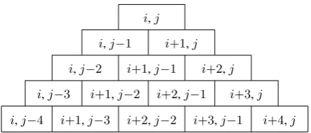
Dynamic programming for context-free inference generally makes use of a chart structure, as shown in Fig. 1. Each cell in the chart represents a pos-sible constituent spanning a substring, which is identified by the indices of the first and last words of the substring. Thus, the cell identified with
i,j i,j−1 i+1,j i,j−2 i+1,j−1 i+2,j i,j−3 i+1,j−2 i+2,j−1 i+3,j i,j−4 i+1,j−3 i+2,j−2 i+3,j−1 i+4,j Figure 1:Fragment of a chart structure. Each cell is indexed with start and end word indices.
i,jwill contain possible constituents spanning the substringwi. . . wj. Context-free inference has
cu-bic complexity in the length of the string n, due to the O(n2) chart cells andO(n) possible child
configurations at each cell. For example, the CYK algorithm, which assumes a grammar in Chomsky Normal Form (hence exactly 2 non-terminal chil-dren for each constituent of span greater than 1), must consider theO(n)possible midpoints for the two children of constituents at each cell.
In a parsing pipeline, some decisions about the hidden structure are made at an earlier stage. For example, base phrase chunking involves identify-ing a span as a base phrase of some category, often NP. A base phrase constituent has no chil-dren other than pre-terminal POS-tags, which all have a single terminal child, i.e., there is no in-ternal structure in the base phrase involving non-POS non-terminals. This has a number of implica-tions for the context-free parser. First, there is no need to build internal structure within the identi-fied base phrase constituent. Second, constituents which cross brackets with the base phrase can-not be part of the final tree structure. This sec-ond constraint on possible trees can be thought of as a constraint on chart cells, as pointed out in Glaysher and Moldovan (2006): no multi-word spanning constituent can begin at a word falling within a base-phrase chunk, other than the first word of that chunk. Similarly, no multi-word span-ning constituent can end at a word falling within a base-phrase chunk, other than the last word of that chunk. These constraints rule out many possible structures that the full context-free parser would have to otherwise consider.
These start and end constraints can be extracted from the output of the chunker, but the chunker is not trained to optimize the accuracy (or the pre-cision) of these particular constraints, rather typi-cally to optimize chunking accuracy. Further, these constraints can apply even for words which fall outside of typical chunks. For example, in En-glish, verbs and prepositions tend to occur before their arguments, hence are often unlikely to end constituents, despite not being inside a typically defined base phrase. If we can build a classifier specifically for this task (determining whether a
Strings in corpus 39832
Word tokens in corpus 950028
Tokens neither first nor last in string 870399
Word tokens inS1 439558 50.5%
Word tokens inE1 646855 74.3%
Table 1:Statistics on word classes from sections 2-21 of the Penn Wall St. Journal Treebank
word can start or end a multi-word constituent), we can more directly optimize the classifier for use within a pipeline.
3 Starting and ending constituents
To better understand the particular task that we propose, and its likely utility, we first look at the distribution of classes and our ability to build sim-ple classifiers to predict these classes. First, let us introduce notation. Given a string ofnwords
w1. . . wn, we will say that a wordwi (1<i<n) is
in the classS>1 if there is a constituent spanning
wi. . . wj for some j>i; andwi ∈ S1 otherwise.
Similarly, we will say that a wordwj (1<j<n) is
in the classE>1 if there is a constituent spanning
wi. . . wj for somei<j; andwj ∈ E1 otherwise.
These are two separate binary classification tasks. Note that the first word w1 and the last word
wnare unambiguous in terms of whether they start
or end constituents of length greater than 1. The first wordw1must start a constituent spanning the
whole string, and the last wordwn must end that
same constituent. The first wordw1 cannot end a
constituent of length greater than 1; similarly, the last word wn cannot start a constituent of length
greater than 1. Hence our classifier evaluation omits those two word positions, leading to n−2
classifications for a string of lengthn.
Table 1 shows statistics from sections 2-21 of the Penn WSJ Treebank (Marcus et al., 1993). From the nearly 1 million words in approximately 40 thousand sentences, just over 870 thousand are neither the first nor the last word in the string, hence possible members of the setsS1 orE1, i.e.,
not beginning a multi-word constituent (S1) or not
ending a multi-word constituent (E1). Of these,
over half (50.5%) do not begin multi-word con-stituents, and nearly three quarters (74.3%) do not end multi-word constituents. This high latter per-centage reflects English right-branching structure.
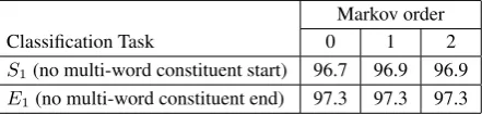
[image:2.595.305.524.71.137.2]fea-Markov order
Classification Task 0 1 2
S1(no multi-word constituent start) 96.7 96.9 96.9
[image:3.595.75.296.72.125.2]E1(no multi-word constituent end) 97.3 97.3 97.3
Table 2: Classification accuracy on development set for bi-nary classesS1andE1, for various Markov orders.
tures similar to those used for NP chunking in Sha and Pereira (2003), including surrounding POS-tags (provided by a separately trained log linear POS-tagger) and surrounding words, up to 2 be-fore and 2 after the current word position.
Table 2 presents classification accuracy on the development set for both of these classification tasks. We trained models with Markov order 0 (each word classified independently), order 1 (fea-tures with class pairs) and order 2 (fea(fea-tures with class triples). This did not change performance for theE1 classification, but Markov order 1 was
slightly (but significantly) better than order 0 for
S1 classification. Hence, from this point forward,
all classification will be Markov order 1.
We can see from these results that simple classi-fication approaches yield very high classiclassi-fication accuracy. The question now becomes, how can classifier output be used to constrain a context-free parser, and what is the impact on parser perfor-mance of using such a classifier in the pipeline.
4 Closing chart cells
Before moving on to an empirical investigation of constraining context-free parsers with the methods we propose, we first need to take a fairly detailed look at representations internal to these parsers. In particular, while we can rule out multi-word con-stituents with particular start and end positions, there may be intermediate orincompletestructures within the parser that should not be ruled out at these same start and end positions. Hence the no-tion of “closing” a chart cell is slightly more com-plicated than it may seem initially.
Consider the chart representation in Fig. 1. Sup-pose thatwi is in classS1 andwj is in classE1,
for i<j. We can “close” all cells(i, k) such that
i<k and all cells (l, j) such that l<j, based on the fact that multi-word constituents cannot begin with word wi and cannot end withwj. A closed
cell will not takecompleteentries, and, depending on the constraint used to close the cell, will have restrictions on incomplete entries. To make this more explicit, let us precisely define complete and incomplete entries.
Context-free inference using dynamic program-ming over a chart structure builds longer-span con-stituents by combining smaller span concon-stituents, guided by rules in a context-free grammar. A context-free grammarG = (V, T, S†, P) consists
of: a set of non-terminal symbols V, including a
special start symbolS†; a set of terminal symbols T; and a set of rule productions P of the form
A → α for A ∈ V and α ∈ (V ∪T)∗, i.e.,
a single non-terminal on the left-hand side of the rule production, and a sequence of 0 or more ter-minals or non-terter-minals on the right-hand side of the rule. If we have a rule productionA → B C
inP, a completed B entry in chart cell(i, j) and a completed C entry in chart cell(j, k), then we can place a completedAentry in chart cell(i, k), typically with some indication that theAwas built from theB andCentries. Such a chart cell entry is sometimes called an “edge”.
The issue with incomplete edges arises when there are rule productions inP with more than two children on the right-hand side of the rule. Rather than trying to combine an arbitrarily large num-ber of smaller cell entries, a more efficient ap-proach, which exploits shared structure between rules, is to only perform pairwise combination, and storeincompleteedges to represent combina-tions that require further combination to achieve a complete edge. This can either be performed in advance, e.g., by factoring a grammar to be in Chomsky Normal Form, as required by the CYK algorithm (Cocke and Schwartz, 1970; Younger, 1967; Kasami, 1965), resulting in “incomplete” non-terminals created by the factorization; or in-complete edges can be represented through so-called dotted rules, as with the Earley (1970) al-gorithm, in which factorization is essentially per-formed on the fly. For example, if we have a rule productionA →B C DinP, a completedB en-try in chart cell(i, j) and a completedC entry in chart cell(j, k), then we can place an incomplete
edgeA→B C·Din chart cell(i, k). The dot sig-nifies the division between what has already been combined (to the left of the dot), and what remains to be combined.1 Then, if we have an incomplete edgeA→ B C·Din chart cell(i, k)and a com-pleteDin cell(k, l), we can place a completedA
entry in chart cell(i, l).
If a chart cell (i, j) has been “closed” due to constraints limiting multi-word constituents with that span – eitherwi ∈S1 orwj ∈E1(andi<j) –
then it is clear that “complete” edges should not be entered in the cell, since these represent precisely the multi-word constituents that are being ruled out. How about incomplete edges? To the extent that an incomplete edge can be extended to a valid complete edge, it should be allowed. There are two cases. Ifwi ∈S1, then under the assumption
that incomplete edges are extended from left-to-right (see footnote 1), the incomplete edge should
Parsing accuracy % of Cells Parsing constraints LR LP F Closed None (baseline) 88.6 89.2 88.9 – S1positions 87.6 89.1 88.3 44.6
E1positions 87.4 88.5 87.9 66.4
[image:4.595.76.290.71.152.2]BothS1andE1 86.5 88.6 87.4 80.3
Table 3:Charniak parsing accuracy on section 24 under var-ious constraint conditions, using word labels extracted using Markov order 1 model.
be discarded, because any completed edges that could result from extending that incomplete edge would have the same start position, i.e., the chart cell would be(i, k)for somek>i, which is closed to the completed edge. However, ifwi 6∈ S1, then
wj ∈E1. A complete edge achieved by extending
the incomplete edge will end atwk for k>j, and
cell(i, k)may be open, hence the incomplete edge should be allowed in cell(i, j). See§6 for limita-tions on how such incomplete edges arise in closed cells, which has consequences for the worst-case complexity under certain conditions.
5 Constraining the Charniak parser 5.1 Parser overview and constraint methods
The Charniak (2000) parser is a multi-stage, agenda-driven, edge-based parser, that can be con-strained by precluding edges from being placed on the agenda. Here we will briefly describe the over-all architecture of that parser, and our method for constraining its search.
The first stage of the Charniak parser uses an agenda and a simple PCFG to build a sparse chart, which is used in later stages with the full model. We will focus on this first stage, since it is here that we will be constraining the parser. The edges on the agenda and in the chart are dotted rules, as described in§4. When edges are created, they are pushed onto the agenda. Edges that are popped from the agenda are placed in the chart, and then combined with other chart entries to create new edges that are pushed onto the agenda. When a complete edge spanning the whole string is placed in the chart, at least one full solution exists in the chart. After this happens, the parser continues adding edges to the chart and agenda until reaching some parameterized target number of additional edges in the chart, at which point the next stage of the pipeline receives the chart as input and any edges remaining on the agenda are discarded.
We constrain the first stage of the Charniak parser as follows. Using classifiers, a subset of word positions are assigned to classS1, and a
sub-set are assigned to class E1. (Words can be
as-signed to both.) When an edge is created for cell
(i, j), wherei < j, it is not placed on the agenda if either of the following two conditions hold: 1)
wi∈S1; or 2) the edge is complete andwj ∈E1.
0.5 0.6 0.7 0.8 0.9 1
0.95 0.96 0.97 0.98 0.99 1
Recall
Precision
Start classification End classification
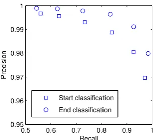
Figure 2:Precision/recall tradeoff ofS1andE1tags on the
development set.
Of course, the output of our classifier is not per-fect, hence imposing these constraints will some-times rule out the true parse, and parser accuracy may degrade. Furthermore, because of the agenda-based heuristic search, the efficiency of search may not be impacted as straightforwardly as one might expect for an exact inference algorithm. For these reasons, we have performed extensive empirical trials under a variety of conditions to try to clearly understand the best practices for using these sorts of constraints for this sort of parser.
5.2 Experimental trials
We begin by simply taking the output of the Markov order 1 taggers, whose accuracies are re-ported in Table 2, and using word positions labeled asS1orE1to “close” cells in the Charniak parser,
as described above. Table 3 presents parser accu-racy on the development set (section 24) under four conditions: the unconstrained baseline; using just
S1 words to close cells; using just E1 word
posi-tions to close cells; and using bothS1andE1
po-sitions to close cells. As can be seen from these results, all of these trials result in a decrease in accuracy from the baseline, with larger decreases associated with higher percentages of closed cells. These results indicate that, despite the relatively high accuracy of classification, the precision of our classifier in producing the S1 and E1 tags is too
low. To remedy this, we traded some recall for pre-cision as follows. We used the forward-backward algorithm with our Markov order 1 tagging model to assign a conditional probability at each word po-sition of the tagsS1 andE1 given the string. At
each word positionwifor1<i<n, we took the log
likelihood ratio of tagS1as follows:
LLR(wi∈S1) = log P(P(wwi∈S1|w1. . . wn)
i6∈S1|w1. . . wn) (1)
and the same for tagE1. A default classification
threshold is to labelS1orE1if the above log
like-lihood is greater than zero, i.e., if theS1tag is more
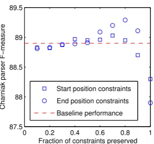
[image:4.595.339.493.73.212.2]0 0.2 0.4 0.6 0.8 1 87.5
88 88.5 89 89.5
Fraction of constraints preserved
Charniak parser F−measure
[image:5.595.106.258.71.212.2]Start position constraints End position constraints Baseline performance
Figure 3: Charniak parser F-measure at various operating points of the fractioncof total constraints kept.
Each word position in a string was ranked with respect to these log likelihood ratios for each tag.2 If the total number of words wi with LLR(wi ∈S1) > 0is k, then we defined
multi-ple operating points by setting the threshold such thatckwords remained above threshold, for some constantcbetween 0 and 1. Fig. 2 shows the pre-cision/recall tradeoff at these operating points for bothS1 andE1 tags. Note that for both tags, we
can achieve over 99% precision with recall above 70%, and for theE1tag (a more frequent class than
S1) that level of precision is achieved with recall
greater than 90%.
Constraints were derived at each of these oper-ating points and used within the Charniak parsing pipeline. Fig. 3 shows the F-measure parsing per-formance using eitherS1 orE1constraints at
vari-ous values ofcfor preservingckof the originalk
constraints. As can be seen from that graph, with improved precision both types of constraints have operating points that achieve accuracy improve-ments over the baseline parser on the dev set under default parser settings.
This accuracy improvement is similar to results obtained in Hollingshead and Roark (2007), where base phrase constraints from a finite-state chun-ker were used to achieve improved parse accuracy. Their explanation for the accuracy improvement, which seems to apply in this case as well, is that the first stage of the Charniak parser is still pass-ing the same number of edges in the chart to the second stage, but that the edges now come from more promising parts of the search space, i.e., the parser does a better job of exploring good parts of the search space. Hence the constraints seem to be doing what they should do, which is constrain the search without unduly excluding good solutions.
Note that these results are all achieved with the default parsing parameterizations, so that ac-curacy gains are achieved, but not necessarily ef-ficiency gains. The Charniak parser allows for 2Perceptron weights were interpreted in the log domain and conditionally normalized appropriately.
0 200 400 600 800 1000 1200 86
87 88 89 90
Seconds to parse development set
F−measure parse accuracy Constrained parser
Unconstrained parser
Figure 4: Speed/accuracy tradeoff for both the uncon-strained Charniak parser and when conuncon-strained with high pre-cision start/end constraints.
narrow search parameterizations, whereby fewer edges are added to the chart in the initial stage. Given the improved search using these constraints, high accuracy may be achieved at far narrower search parameterizations than the default setting of the parser. To look at potential efficiency gains to be had from these constraints, we chose the most constrained operating points for both start and end constraints that do not hurt accuracy rel-ative to the baseline parser (c = 0.7 for S1 and
c= 0.8forE1) and used both kinds of constraints
in the parser. We then ran the Charniak parser with varying search parameters, to observe performance when search is narrower than the default. Fig. 4 presents F-measure accuracy for both constrained and unconstrained parser configurations at various search parameterizations. The times for the con-strained parser configurations include the approx-imately 20 seconds required for POS-tagging and word-boundary classification of the dev set.
These results demonstrate a sharper knee of the curve for the constrained runs, with parser accu-racy that is above that achieved by the uncon-strained parser under the default search parameter-ization, even after a nearly 5 times speedup.
5.3 Analysis of constraints on 1-best parses
[image:5.595.338.489.73.197.2]er-rors, but also eliminated some MAP parses. To get a sense of how often search errors were corrected versus ruling out of MAP parses, we compared the constrained and unconstrained parses at each string, and tallied when the uncon-strained parse probabilities were greater (or less) than the constrained parse probabilities, as well as when they were equal. At the default search pa-rameterization (210), 84.8 percent of the strings had the same parses; in 9.2 percent of the cases the unconstrained parses had higher probability; and in 5.9 percent of the cases the constrained parses had higher probability. The narrower search pa-rameterization at the knee of the curve in Fig. 4 had similar results: 84.6 percent were the same; in 8.6 percent of the cases the unconstrained probability was higher; and in 6.8 percent of the cases the con-strained probability was higher. Hence, when the 1-best parse differs, the parse found via constraints has a higher probability in approximately 40 per-cent of the cases.
6 O(n2)complexity context-free parsing
Using sufficientS1 andE1 constraints of the sort
we have been investigating, we can achieve worst-case quadratic (instead of cubic) complexity. A proof, based on the CYK algorithm, is given in Appendix A, but we can make the key points here. First, cubic complexity of context-free inference is due to O(n2) chart cells and O(n) possible
child configurations per cell. If we “close” all but
O(n)cells, the “open” cells will be processed with worst-case quadratic complexity (O(n)cells with
O(n)possible child configurations per cell). If we can show that the remainingO(n2) “closed” cells
each can be processed within constant time, then the overall complexity is quadratic. The proof in Appendix A shows that this is the case if closing a cell is such that: when a cell(i, j)is closed, then either all cells(i, k)fork>iare closed or all cells
(k, j) for k<j are closed. These conditions are achieved when we select setsS1 andE1and close
cells accordingly.
Just as we were able to order word position log likelihood scores for classes S1 and E1 to
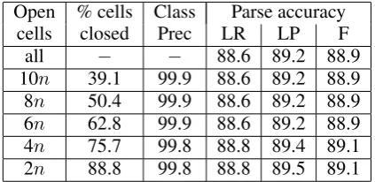
im-prove precision in the previous section, here we will order them so that we can continue select-ing positions until we have guaranteed less than some threshold of “open” cells. If the threshold is linear in the length of the string, we will be able to parse the string with worst-case quadratic complexity, as shown in Appendix A. We will set our threshold to kn for some constant k (in our experiments, k ranges from 2 to 10). Table 4 presents the percentage of cells closed, class (S1
and E1) precision and parser accuracy when the
number of “open” cells is bounded to be less than
Open % cells Class Parse accuracy
cells closed Prec LR LP F
all − − 88.6 89.2 88.9
[image:6.595.310.522.71.174.2]10n 39.1 99.9 88.6 89.2 88.9 8n 50.4 99.9 88.6 89.2 88.9 6n 62.8 99.9 88.6 89.2 88.9 4n 75.7 99.8 88.8 89.4 89.1 2n 88.8 99.8 88.8 89.5 89.1 Table 4: Varying constantkforkn“open” cells, yielding O(n2) parsing complexity guarantees
the threshold. These results clearly demonstrate that such constraints can be placed on real context-free parsing problems without significant impact to accuracy–in fact, with small improvements.
We were quite surprised by these trials, fully ex-pecting these limits to negatively impact accuracy. The likely explanation is that the existing Char-niak search strategy itself is bounding processing in such a way that the additional constraints placed on the process do not interfere with standard pro-cessing. Note that our approach closes a higher percentage of cells in longer strings, which the Charniak pipeline already more severely prunes than shorter strings. Further, this approach appears to be relying very heavily onE1constraints, hence
has very high precision of classification.
While the Charniak parser may not be the ideal framework within which to illustrate these worst-case complexity improvements, the lack of impair-ment to the parser provides strong evidence that other parsers could make use of the resulting charts to achieve significant efficiency gains.
7 Conclusion & Future Work
In this paper, we have presented a very simple ap-proach to constraining context-free chart parsing pipelines that has several nice properties. First, it is based on a simple classification task that can achieve very high accuracy using very sim-ple models. Second, the classifier output can be straightforwardly used to constrain any chart-based context-free parser. Finally, we have shown (in Appendix A) that “closing” sufficient cells with these techniques leads to quadratic worst-case complexity bounds. Our empirical results with the Charniak parser demonstrated that our classifiers were sufficiently accurate to allow for such bounds to be placed on the parser without hurting parsing accuracy.
CYK(w1. . . wn, G= (V, T, S†, P, ρ)) PCFGGmust be in CNF
1 for t = 1tondo scan in words/POS-tags (span=1)
2 for j = 1to|V|do
3 αj(t, t)←P(Aj→wt)
4 for s = 2tondo all spans>1
5 for t = 1ton−s+1do
6 e←t+s−1 end word position for this span
7 for i = 1to|V|do
8 ζi(t, e)←argmax
t<m≤e
„ argmax
j,k P(Ai→AjAk)αj(t, m−1)αk(m, e)
«
9 αi(t, e)← max
t<m≤e
„ max
j,k P(Ai→AjAk)αj(t, m−1)αk(m, e)
«
Figure 5:Pseudocode of a basic CYK algorithm for PCFG in Chomsky Normal Form (CNF).
References
Charniak, E. and M. Johnson. 2005. Coarse-to-finen-best parsing and MaxEnt discriminative reranking. In Proceed-ings of the 43rd Annual Meeting of the Association for Computational Linguistics (ACL), pages 173–180. Charniak, E. 2000. A maximum-entropy-inspired parser. In
Proceedings of the 1st Conference of the North American Chapter of the Association for Computational Linguistics, pages 132–139.
Cocke, J. and J.T. Schwartz. 1970. Programming languages and their compilers: Preliminary notes. Technical report, Courant Institute of Mathematical Sciences, NYU. Collins, M.J. 2002. Discriminative training methods for
hid-den Markov models: Theory and experiments with per-ceptron algorithms. In Proceedings of the Conference on Empirical Methods in Natural Language Processing (EMNLP), pages 1–8.
Earley, J. 1970. An efficient context-free parsing algorithm.
Communications of the ACM, 6(8):451–455.
Glaysher, E. and D. Moldovan. 2006. Speeding up full syn-tactic parsing by leveraging partial parsing decisions. In
Proceedings of the COLING/ACL 2006 Main Conference Poster Sessions, pages 295–300.
Hollingshead, K. and B. Roark. 2007. Pipeline iteration. In
Proceedings of the 45th Annual Meeting of the Association for Computational Linguistics (ACL), pages 952–959. Kasami, T. 1965. An efficient recognition and syntax
analysis algorithm for context-free languages. Technical report, AFCRL-65-758, Air Force Cambridge Research Lab., Bedford, MA.
Marcus, M.P., M.A. Marcinkiewicz, and B. Santorini. 1993. Building a large annotated corpus of English: The Penn treebank.Computational Linguistics, 19:313–330. Ratnaparkhi, A. 1999. Learning to parse natural language
with maximum entropy models. Machine Learning, 34(1-3):151–175.
Sha, F. and F. Pereira. 2003. Shallow parsing with con-ditional random fields. InProceedings of HLT-NAACL, pages 134–141.
Younger, D.H. 1967. Recognition and parsing of context-free languages in time n3. Information and Control,
10(2):189–208.
Appendix A Proof of quadratic complexity parsing with constraints
For this proof, we will use the well-known CYK parsing algorithm, which makes use of grammars in Chomsky Normal Form (CNF). To achieve CNF, among other things, rules with more than 2
children on the right-hand side must be factored into multiple binary rules. To do this, compos-ite non-terminals are created in the factorizations, which represent incomplete constituents, i.e., those edges that require further combination to be made complete.3 For example, if we have a rule pro-ductionA →B C Din the context-free grammar
G, then a new composite non-terminal would be created, e.g.,B-C, and two binary rules would re-place the previous ternary rule: A→B-C Dand
B-C → B C. TheB-C non-terminal represents part of a rule expansion that needs to be combined with something else to produce a complete non-terminal from the original set of non-non-terminals. Let V0 be the set of non-terminals that are
cre-ated through factorization, which hence represent incomplete edges.
Fig. 5 shows pseudocode of a basic CYK algo-rithm for use with a probabilistic CFG in CNF,
G = (V, T, S†, P, ρ). The function ρ maps from
rules inP to probabilities. Lines 1-3 of the algo-rithm in Fig. 5 initialize the span 1 cells. Lines 4-9 are where the cubic complexity comes in: O(n)
loops in line 4, each of which includeO(n)loops in line 5, each of which requires finding a max-imum over O(n) midpoints m in lines 8-9. For each non-terminalAi ∈ V at each cell(t, e), the
algorithm stores a backpointerζi(t, e)in line 8, for
efficiently extracting the maximum likelihood so-lution at the end of inference; and maximum prob-abilitiesαi(t, e) in line 9, for use in the dynamic
program.
Given a set of word positions in the classesS1
andE1, as defined in the main part of this paper,
we can designate all cells(i, j)in the chart where eitherwi ∈ S1 orwj ∈ E1 to be “closed”. Chart
cells that are not closed will be called “open”. The total number of cells in the chart is (n2 +n)/2,
and if we set a threshold on the maximum number of open cells to bekn, the number of closed cells must be at least(n2+n)/2−kn. Given an ordering
QUADCYK(w1. . . wn, G= (V, T, S†, P, ρ), V0, S1, E1) PCFGGmust be in CNF
1 for t = 1tondo scan in words/POS-tags (span=1)
2 for j = 1to|V|do
3 αj(t, t)←P(Aj→wt)
4 for s = 2tondo all spans>1
5 for t = 1ton−s+1do
6 e←t+s−1 end word position for this span
7 if wt∈S1 CONTINUE start positiont“closed”
8 else if we∈E1 end positione“closed”
9 for i = 1to|V|do
10 ifAi6∈V0 CONTINUE only “incomplete” factored non-terminals (V0)
11 ζi(t, e)←argmax
j,k P(Ai→AjAk)αj(t, e−1)αk(e, e)
12 αi(t, e)← max
j,k P(Ai→AjAk)αj(t, e−1)αk(e, e)
13 else chart cell(t, e)“open”
14 for i = 1to|V|do
15 ζi(t, e)←argmax
t<m≤e
„ argmax
j,k P(Ai→AjAk)αj(t, m−1)αk(m, e)
«
16 αi(t, e)← max
t<m≤e
„ max
j,k P(Ai→AjAk)αj(t, m−1)αk(m, e)
[image:8.595.76.479.69.275.2]«
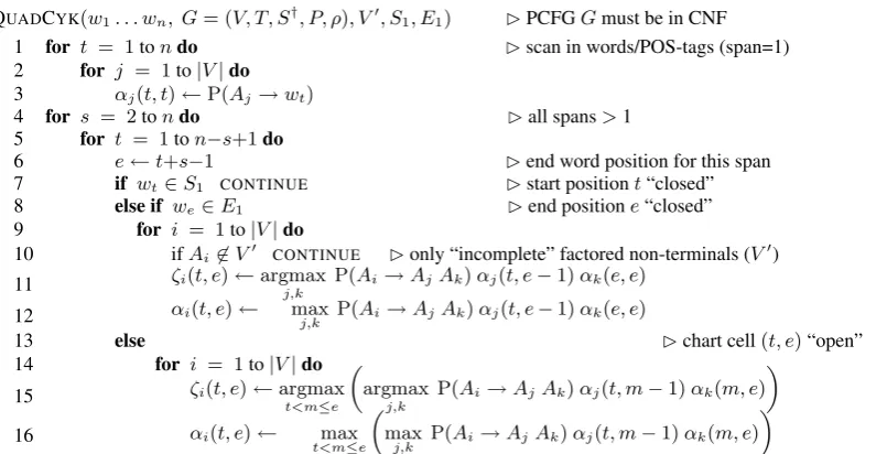
Figure 6: Pseudocode of a modified CYK algorithm, with quadratic worst case complexity withO(n)“open” cells. In addition to string and grammar, it requires specification of factored non-terminal setV0and position constraints (S
1, E1).
related cells, until the requisite number of closures are achieved. Then the resulting sets ofS1 word
positions andE1word positions can be provided to
the parsing algorithm, in addition to the grammar
Gand the set of factored non-terminalsV0.
Fig. 6 shows pseudocode of a modified CYK al-gorithm that takes into account S1 and E1 word
classes. Lines 1-6 of the algorithm in Fig. 6 are identical to those in the algorithm in Fig. 5. At line 7, we have identified the chart cell being pro-cessed, which is(t, e). Ifwt∈ S1 then the cell is
completely closed, and there is nothing to do. Oth-erwise, ifwe ∈E1(lines 8-12), then factored
non-terminals from V0 can be created in that cell by
finding legal combinations of children categories. If neither of these conditions hold, then the cell is open (lines 13-16) and processing occurs as in the standard CYK algorithm (lines 14-16 of the algo-rithm in Fig. 6 are identical to lines 7-9 in Fig. 5).
If the number of “open” cells is less thanknfor some constantk, then we can prove that the algo-rithm in Fig. 6 isO(n2)when given a left-factored
grammar in CNF. A key part of the proof rests on two lemmas:
Lemma 1: LetV0 be the set of composite
non-terminals created when left-factoring a CFG to be in CNF, as described earlier. Then, for
any productionAi→ AjAkin the grammar,
Ak6∈V0.
Proof: With left-factoring, any k-ary production
A→ A1. . . Ak−1Akresults in new non-terminals
that concatenate the first k−1 non-terminals on the right-hand side. These factored non-terminals are always the leftmost child in the new produc-tion, hence no second child in the resulting CNF grammar can be a factored non-terminal.2
Lemma 2: For a cell (t, e) in the chart, if
we ∈ E1, then the only possible midpointm for creating an entry in the cell ise.
Proof:Placing an entry in cell(t, e)requires a rule
Ai → AjAk, anAjentry in cell(t, m−1)and an
Akentry in cell(m, e). Suppose there is anAk
en-try in cell(m, e)form < e. Recall thatwe ∈E1,
hence the cell(m, e)is closed to non-terminals not inV0. By Lemma 1, A
k 6∈ V0, therefore the cell
(m, e)is closed toAkentries. This is a
contradic-tion. Therefore, the lemma is proved.2
Theorem: LetObe the set of cells(t, e)such that wt 6∈ S1 and we 6∈ E1 (“open” cells). If|O| < knfor some constantk, wherenis the length of the string, then the algorithm in Fig. 6 has worst case complexityO(n2).
Proof: Lines 4 and 5 of the algorithm in Fig. 6
loop throughO(n2)cells(t, e), for which there are
three cases: wt ∈ S1 (line 7 of Fig. 6); we ∈ E1
(lines 8-12); and(t, e)∈ O(lines 13-16).
Case 1:wt∈S1. No further work to be done.
Case 2: we ∈ E1. There is a constant amount of
work to be done, for the reason that there is only one possible midpointmfor binary children com-binations (namelye, as proved in Lemma 2), hence no need to perform the maximization over O(n)
midpoints.
Case 3: (t, e) ∈ O. As with standard CYK pro-cessing, there areO(n)possible midpointsmover which to maximize, henceO(n)work required.
Only O(n) cells fall in case 3, hence the to-tal amount of work associated with the cells inO isO(n2). There are O(n2) cells associated with
cases 1 and 2, each of which has a total amount of work bounded by a constant, hence the total amount of work associated with the cells not in Ois alsoO(n2). Therefore the overall worst-case