Methods of analysis of geomagnetic field variations and cosmic ray data

(1)

L E T T E R

Open Access

Methods of analysis of geomagnetic field

variations and cosmic ray data

Oksana V Mandrikova

1,2,3*

, Igor S Solovev

1,2,3

and Timur L Zalyaev

1

Abstract

In the present paper, we propose a wavelet-based method of describing variations in the Earth’s magnetic field, such as the horizontal component of the geomagnetic field, in addition to methods for evaluating changes in the energy characteristics of the field and for isolating the periods of increased geomagnetic activity. Based on a combination of multiresolution wavelet decompositions with neural networks, we propose a method of approximation of the cosmic ray time course and the allocation of anomalous variations (Forbush effects) that occur during periods of high solar activity. During the realization of the method, an algorithm was created for selecting the level of the wavelet decomposition and adaptive construction of the neural network. By using the proposed methods, we performed a joint analysis of the geomagnetic field and cosmic rays during periods of strong magnetic storms. The strongest geomagnetic field perturbations were observed in periods of abnormal changes in cosmic ray level. Assessment of the intensity of geomagnetic disturbances on the eve of and during magnetic storm development allowed us to highlight local increases in intensity of the geomagnetic field occurring at different frequency ranges prior to the development of the storm’s main phase. Implementation of the proposed method with theoretical tools in combination with other methods will improve the estimation accuracy of the geomagnetic field state during space weather forecasting.

Keywords:Geomagnetic field; Cosmic rays; Wavelet transform; Neural networks; Magnetic storms

Findings

Introduction

The present study examines the processes that occur in circumterrestrial space during magnetic perturbations by creating new algorithms and techniques for recognition, analysis, and interpretation of data. During perturbed periods, parameters determined by special equipment in-clude a complex non-stationary structure that contains non-smooth local features arising at random time points that carry information about the processes under study. A lack of theoretical basis for providing adequate presenta-tion of data for analysis leads to inevitable loss and distor-tion of informadistor-tion and requires the applicadistor-tion of contemporary techniques such as pattern recognition and digital signal processing (Nayar et al. 2006; Hafez et al.

2013; Xu et al. 2008; Jach et al. 2006; Paschalis et al. 2013; Macpherson et al. 2001; Woolley et al. 2010; Soloviev et al. 2012; Rotanova et al. 2004).

During periods of magnetic storms in the recorded geo-magnetic data, variations occur among frequency ranges. The emerging local structures are determined by field per-turbations and reveal the intensity and nature of the devel-opment of a magnetic storm. The complex structure of geomagnetic data limits the abilities of spectral analysis methods by failing to provide information on the local changes occurring in the physical process and their scale characteristics.

The disadvantages of these methods also include limi-tations in identifying and interpreting hidden patterns in the behavior of the data. In the present study, wavelet transform is suggested for analysis of geomagnetic data because such methods allow detection of several inter-esting deterministic and more stochastic features in the time series of solar activity indicators (Lundstedt et al. 2005). Wavelet transform is the underlying mathematical tool used for analyzing local features occurring in the * Correspondence:[email protected]

1

Institute of Cosmophysical Researches and Radio Wave Propagation, Mirnaya Str., 7, Kamchatka Region, Elizovskiy District, Paratunka 684034, Russia 2

Kamchatka State Technical University, Klyuchevskaya Street 35, 683003 Petropavlovsk-Kamchatsky, Russia

Full list of author information is available at the end of the article

(2)

geomagnetic field during intense solar flares (Ivanov et al. 2001; Rotanova et al. 2004; Nayar et al. 2006) and for de-veloping algorithms for automatic determination of the onset of a magnetic storm (Hafez et al. 2013). Further-more, the wavelet transform is a powerful tool for elimin-ating noise and excluding the periodic component caused by the Earth’s rotation (Xu et al. 2008; Jach et al. 2006). A method used for allocation of anomalies in geomagnetic data was developed on the basis of the wavelet transform (Zaourar et al. 2013). The authors of the present paper created technology for automatic extraction of the unper-turbed level of the horizontal component of the geomag-netic field based for the first time on wavelet transform (Mandrikova et al. 2013). This method has significantly reduced error in automatic calculation of the K-index in comparison to the adaptative smoothing method (KASm) recommended by the International Real-Time Magnetic Observatory Network (Intermagnet) and currently used by Paratunka Observatory, Kamchatka Region, Institute of Cosmophysical Researches and Radiowave Propagation, Far Eastern Branch of the Russian Academy of Sciences (IKIR FEB RAS), and Yakutsk Observatory, Yakutsk, Institute of Cosmophysical Research and Aeronomy, Siberian Branch, Russian Academy of Sciences (IKFIA SB RAS). In the present paper, the authors suggest a new technique for determining variation in the geomagnetic field by using the H-component and present related methods of extracting geomagnetic perturbations, esti-mating their intensity, and determining periods of in-creased geomagnetic activity. The suggested theoretical tools can be implemented in the automatic mode, which is close to the real-time mode and can be adapted to vari-ous magnetic observatories.

The topology of the geomagnetic field during magnetic storms is characterized by variability of cosmic rays on the Earth’s surface (Kozlov and Markov 2007), which present an integral result of various solar, heliospheric, and atmospheric phenomena with a complex structure. The most substantial changes in cosmic ray parameter are caused by emissions of the corona substance and subsequent changes in parameters of the interplanetary field and solar wind (Vecchio et al. 2012). The current study of the dynamics of cosmic ray flux includes methods of adaptive approximation, wavelet transform, and neural networks. Using neural networks for the primary pro-cessing of neutron monitor data have led to greater ef-ficiency in the noise reduction procedure compared with median methods (Paschalis et al. 2013). Neural networks also can be used to detect abnormal features in complex functions. For example, the method of automatic detec-tion of sudden commencement is based on neural net-works (Segarra and Curto 2013). Based on a combination of wavelet transform and empirical mode decompos-ition, the dominant temporal scales of long-term temporal

variation of cosmic rays were highlighted for periods of 11, 22, and 6 years and biennial oscillation, and their phys-ical nature was determined (Vecchio et al. 2012). In the present study, the authors combine multiscale wavelet transforms and neural networks to develop a technique for approximating the time variation of cosmic rays and discovering anomalous changes connected with increased solar activity.

This method enables noise suppression to distinguish characteristic variations and to examine the details of their structures.

On the basis of the proposed methods, we have per-formed joint analysis of the geomagnetic field and cos-mic rays during periods of strong magnetic storms on 5 to 7 April 2010 and 5 September 2012. During the analysis, we used 1-min geomagnetic field data from Intermagnet (www.intermagnet.org) and 1-min neutron monitor data obtained within the framework of the Real-time Neutron Monitor Database (NMDB) (www.nmdb.eu/) project.

Description of methods

Decomposition of time series into components based on wavelet transform

Having the discrete function value fj (i.e., values of

the function at the grid with a resolution of 2−j), we can consider the following subspace as the sampling space:

Vj¼closL2_{ð Þ}_R ϕ 2jt−n

;n∈Z; ð1Þ

whereVjis generated by translation and dilation ofthe scaling function ϕ (Daubechies 1992; Chui 1992; Mallat 1999), andL2(R) is the Lebesgue space.

By performing the projection of fj into spaces Vj −1

and Wj −1, we obtain (Daubechies 1992; Chui 1992;

Mallat 1999)

Vj¼Vj−1⊕Wj−1; ð2Þ

where⊕denotes the orthogonal sum. The set of func-tions (wavelets)Ψj,n=2j/2Ψ(2jt−n),n∈Zform the basis of the spaceWj.

We considerfjas time series. On the basis of Equation 2,

the time series can be represented as:

f_jð Þ ¼t f_j−₁ð Þ þt g_j−₁ð Þt : ð3Þ

Mandrikovaet al. Earth, Planets and Space2014,66:148 Page 2 of 17

(3)

Figure 1Graphic representation of wavelet packet decomposition to the levelmof the time seriesfj.

(4)

Figure 3(See legend on next page.)

(5)

defined by the sequence of coefficientscj_¼ _c

j;n _n_∈_Z∈Vj

anddj¼ dj;n

n∈Z∈Wj:cj,n=〈f,ϕj,n〉,dj,n=〈f,Ψj,n〉.

The described computational procedure is known as a wavelet decomposition algorithm, which can be applied to any resolution (scale) j of the signal (Daubechies 1992; Chui 1992; Mallat 1999).

If this decomposition procedure is performed on the time seriesfj(t)mtimes, we obtain the following form of

the decomposition of the spaceVj:

Vj¼Wj−1⊕Wj−2⊕…⊕Wj−m⊕Vj−m: ð4Þ

As a result, the time seriesfj(t) can be represented as

the sum of the components listed below:

f_jð Þ ¼t g_j−₁ð Þ þt g_j−₂ð Þ þt …þg_j−mð Þ þt f_j−mð Þt

Component gjis known as a detailed (high-frequency)

component of the time series; componentfj− mis known

as the smoothed component of the time series.

In the wavelet transform theory, decomposition of the form in Equation 5 is known as multiresolution wavelet decomposition to the level m(Chui 1992; Mallat 1999).

If we apply this space decomposition procedure to the space Wj, we obtain a partition of the high-frequency

components, which allows us to identify different types of time-frequency structures. In the wavelet transform theory, decomposition of fjbased on recursive splitting

of the spaces Vj and Wj is known as the wavelet packet decomposition. Graphic representation of wavelet packet decomposition of the time series fj is shown in

Figure 1.

Description of geomagnetic field variations on the basis of wavelets

Asfj(t), we could consider the time variation of the

hori-zontal component of the geomagnetic field. Without loss of generality, we assume thatj= 0, i.e., the space of initial data is V0¼closL2_{ð Þ}_Rðϕð20t−nÞÞ. Based on the wavelet

packet decomposition, we obtain the following representa-tion off0(t): whereIis a set of indices.

In our previous research (Mandrikova et al. 2013; Mandrikova and Solovev 2013), we showed, that, for Kamchatka and Yakutsk regions, component

f_trendð Þ ¼t X n

c−6;nϕ−6;nð Þt describes the undisturbed level

of the horizontal component of the magnetic field of the Earth, and component f_distð Þ ¼t X

periods of increasing geomagnetic activity. The com-ponent e tð Þ ¼X magnetic disturbance of the component gj(t) on the

scale j (Mandrikova et al. 2013; Mandrikova and Solovev 2013). We used the following criteria to determine the set of indicesI(Mandrikova et al. 2013):

j∈I;ifm Av_j >m Ak_j þε; ð7Þ wheremis the sample mean,vis the index of disturbed field variation,kis the index of calm field variation, andε is a positive number.

Assuming that variableAjkis normally distributed with

some meanμkand varianceσ2,k, it is possible to estimate

εas^ε¼x1−α

Estimation of the set of indices I, particularly for the station Paratunka (Kamchatka Region), was performed using geomagnetic data for 2002, 2005, and 2008, con-taining 63 disturbed field variations and 64 calm field variations.

(See figure on previous page.)

(6)

(7)

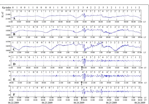
Figure 2 shows geomagnetic data processing results from stations Paratunka (Kamchatka Region), Yakutsk (Yakutsk), and Novosibirsk (Novosibirsk) for the duration of a magnetic storm that occurred 24 to 25 June 2009. The disturbed component of the geomagnetic field, allocated on the basis of the proposed model, describes the power of disturbance of the field and allows us to register the mo-ments of increasing geomagnetic activity on the eve of and during the storms. Analysis of Figure 2 showed an increase in geomagnetic activity from 4:18 to 4:54 UT at all analyzed stations, indicating the beginning of a magnetic storm. The moments of enhancements in geomagnetic activity in Figure 2D,E,F are indicated with arrows. The maximum values of the amplitude of the disturbed component were recorded from approximately 06:08 to 06:27 UT.

Let us consider three possible states of the geomag-netic field: stateh0: calm field; stateh1: weakly perturbed

field; stateh2: perturbed field. According to the proposed

field states, we introduce the following states of the coef-ficientsdj,non the scalej:

hj0: calm coefficient

hj1: weakly perturbed coefficient hj2: perturbed coefficient.

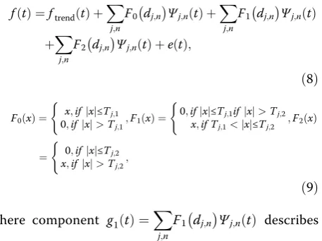
As a measure of magnetic disturbance of the coeffi-cient, it is logical to determine its amplitude. Then, in accordance with the introduced states of the coefficients from Equation 6, we obtain the following representation of geomagnetic field variations:

weak geomagnetic perturbations, where the coefficients

of g1(t) are in a weakly perturbed state; component g₂ð Þ ¼t X Tj,1is considered as quiet.

Threshold functionsF0(x),F1(x), andF2(x) in Equation 9

determine rules for decision-making of coefficient state. Threshold Tj,1 and Tj,2 divide the space of

coeffi-cients X into three disjoint regions X0, X1, and X2.

Then, the rule of decision-making establishes a cor-respondence between decisions of the state of coeffi-cients and regions.

Due to the random nature of the investigated object, the use of any rule was inevitably linked to the possibil-ity of wrong decisions. By using certain rules for select-ing a decision for a given state hji, the average value of

the loss can be defined as (Levin 1963)

Ji_jð Þ ¼x X tional probability that the sample falls into the areaXlif the real state ishji, i≠l i. l is the state of indices, where sign‘/’means conditional probability.

By averaging the conditional risk function over all stateshji,i= 0, 1, 2, we obtain average risk (Levin 1963):

The best rule is the one for which the average risk is smallest (Levin 1963).

Since we did not know the a priori distribution of states

pi, we used a posteriori risk for choosing the best decision

rule (Levin 1963). Posterior probabilities P{hji/x},i= 0, 1, 2,

represent the most complete characterization of the states

hjiwith available priori data.

For simple loss function:

Πil¼ 1₀;_;_ii_¼≠_ll_{; :};

ð12Þ

A posteriori riskJl(x) is (See figure on previous page.)

(8)

(9)

Jlð Þ ¼x

In this case, the criterion of the quality of decision-making is the criterion of the lowest error rate.

Thresholds Tj,1 and Tj,2 are determined by best

deci-sion rule of the decideci-sion-making, ensuring the lowest value of the posterior riskJl(x).

By minimizing the posteriori risk Jl(x), we determine

thresholds Tj,1 and Tj,2, j ∈ I for regions of Kamchatka

and Yakutsk (Mandrikova et al. 2013; Mandrikova and Solovev 2013). The criterion of assessment of the coeffi-cients is the K-index (Bartels et al. 1939). The following assessments were considered:

1) Coefficient belongs to areaX0(i.e., they are in a quiescent state) if the current value of the K-index is 0 or 1;

2) Coefficient belongs to areaX1(i.e., they are in a weakly perturbed state) if the current value of the K-index is 2, 3, or 4;

3) Coefficient belongs to areaX2(i.e., they are in a perturbed state) if the current value of the K-index is more than 4.

The introduced states of coefficients describe the states of the geomagnetic field and their assessment based on the obtained rule for decision-making, which allows us to register moments of increasing geomagnetic activity. In our previous paper (Mandrikova et al. 2013), we developed an automatic algorithm to construct the Sq-curve and to calculate the K-index on the basis of this representation of geomagnetic field variations (shown in Equation 8), and we demonstrated that its application for stations Paratunka and Yakutsk significantly reduced the error of K-index computation in the automatic mode, in comparison with the methodology used in the Intermagnet network stations. In the present work (‘Assessment of changes of energy characteristics of the field and the allocation of periods of increased geomagnetic activity’ subsection), we used this approach to suggest computa-tional solutions for estimating changes in the energy char-acteristics of the field and the allocation of periods of increased geomagnetic activity. To obtain more detailed in-formation on the state of the geomagnetic field, we used continuous wavelet transform.

Assessment of changes of energy characteristics of the field and the allocation of periods of increased geomagnetic activity

For each of the basic wavelet, the continuous wavelet transform is defined by (Daubechies 1992; Chui 1992)

WΨf (b, a) describe the properties of the function f in the neighborhoodbwhen the scale atends to be zero. This property of the continuous wavelet transform allows us to obtain detailed information on the local properties of the functionf.

Using equivalence of discrete and continuous wavelet transforms (Mallat 1999; Chui 1992), it is possible to introduce a method for calculating the intensity of geo-magnetic perturbations at the time point t=b on the scalea. This intensity can be written as:

eb;a¼jðWΨfÞðb;aÞj ð15Þ

Then, by applying a threshold function to the value

eb,a, we can estimate the state of the coefficients and

allocate time-frequency intervals containing weak and strong geomagnetic disturbances on the analyzed scalea:

PTa;1 eb;a where the threshold Ta,1 allows to us allocate weak

and strong perturbations, and the threshold Ta,2

indi-cates strong perturbations.

On the basis of (Equation 15), the intensity of field dis-turbances at the time momentt=bis

Eb ¼ X

a

eb;a ð17Þ

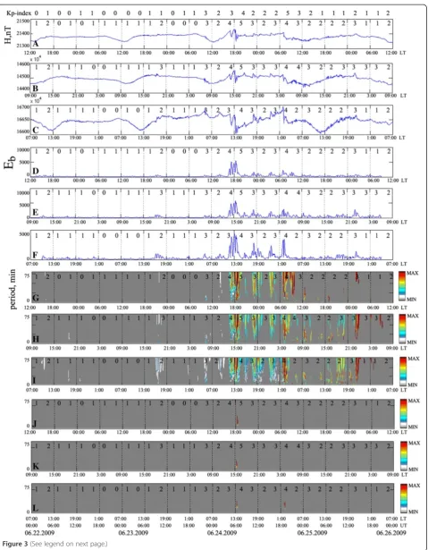
Figure 3 shows the results of assessment of the intensity of geomagnetic disturbances and allocation of periods of

(10)

(11)

increased of geomagnetic activity during a magnetic storm occurring on 24 to 25 June 2009. We estimated thresholds

Ta,1andTa,2by minimizing a posteriori risk, in accordance

with rule of decision-making introduced in ‘Description of geomagnetic field variations on the basis of wavelets’ subsection. K-index was the criterion of estimation of the state of coefficients, where the data used was from stations Paratunka, Yakutsk, and Novosibirsk. Analysis of Figure 3 shows the complex multiscale nature of the process. The results of processing of the data allow us to allocate its gen-eral features. Prior to the beginning of the storm, from about 09:00 to 10:40 UT and 21:30 to 23:30 UT on 23 June and from 02:00 to 03:30 UT on 24 June, local increases in the intensity of geomagnetic disturbances were observed at all analyzed stations, and periods of weak geomagnetic ac-tivity had been formed. Simultaneous occurrence of distur-bances at different stations eliminates the influence of the noise factor and confirms their solar nature. The strongest field perturbations observed from 4:57 to 06:43 UT coin-cide with the moments of the main phase of the storm.

Method of approximation of the time variation of cosmic rays and allocation of anomalous changes in its dynamic on the basis of combination of multiresolution wavelet decompositions and neural networks

We consider the time variation of cosmic rays as fj(t).

Let us assume that the initial data space isV0¼closL2_{ð Þ}_R ϕ_ð20_t₋_n_Þ

ð Þ(i.e.,j= 0).

By performing multiresolution wavelet decomposition of the function f0(t) to the level m, we obtain its

repre-sentation in the following form (see Equation 5):

f₀ð Þ ¼t g₋₁ð Þ þt g₋₂ð Þ þt …þg_−mð Þ þt f_−mð Þt

¼X−m

j¼−1

X

n

dj;nΨj;nð Þ þt X

n

c−m;nϕ−m;nð Þt : ð18Þ

For the smooth componentf₋_mð Þ ¼t X n

c−m;nϕ−m:nð Þt ,

we perform the operation of wavelet reconstruction:

fð₀−mÞð Þ ¼t X

n

cð₀−m_;_nÞϕ0;nð Þt ; ð19Þ

where the upper index (−m) corresponds to the reso-lution of the component before the operation of the wavelet reconstruction.

Further, on the basis of the neural network for re-constructed components, we re-constructed the follow-ing mappfollow-ing:

y:fð₀−mÞ→f₀ð−mÞ ð20Þ To construct the mapping, we used a feedforward neural network with variable structure, which is a net-work in which the structure is determined by minimiz-ing the error on the trainminimiz-ing set. The trainminimiz-ing set is formed from the data registered during quiet periods. In this case, the trained neural network reproduced regular variations of the data being approximated, which is typ-ical for quiet conditions. Network training was performed on the basis of the back error propagation algorithm (Haykin 1999).

If in constructed mapping,^f₀ð−mÞis the actual output of the network andf0*(−m)is desired, thenf0*(−m)=y(f0(−m)) is

an unknown function, and ^f₀ð−mÞ is its approximation, which is reproduced by the neural network. The advantage of the neural network representation of the approximated function is greater flexibility of the basic functions and their ability to adapt (Haykin 1999). When the input of the trained network is the function values from the inter-val [tn−Q+1,tn], the network is able to calculate the

pre-emption of its value in the time interval [tn +1, tn+I],

wheretnis the current discrete time, andIis the length of

the preemption interval.

Network error(approximation error) at time momenttn

is determined as the difference between the desiredf0*(−m)

and actual^f₀ð−mÞoutput values of the function:

em½ ¼tn XI

i¼1

f₀_;ð_i−mÞ½ tn−^f0;ði−mÞ½ tn

; ð21Þ

where i is the step of the feedforward network of the data, and square brackets denote the discrete time.

The algorithm for constructing the network and choosing the level of the wavelet decomposition, based on minimization of the approximation error, is listed below.

If anomalous variations occur in the time variations of the data, the absolute value of the network error would increase. Therefore, the allocation of anomalous changes

(12)

(13)

in the dynamics of the time series could be based, for example, on verifying the condition:

Em;U¼_U1

XU

n¼1

em½ tn >T; ð22Þ

whereUis the length of the observation window, and

Tis a preassigned threshold.

Algorithm for constructing a neural network and choosing the level wavelet decomposition

Step 1. We obtain representation of a smoothed compo-nent of the series in the formfð₀−mÞð Þ ¼t X

n

cð₀−_;_nmÞϕ₀_;_nð Þt ,

wherem= 1.

Step 2. Data array {c0,n(−m)}n=1N , whereNis the array length

and is divided into blocks of {c0,n(−m)}n=1Q , {c0,n(−m)}n=2Q+1,…,

{c0,n(−m)}n=NN −Q+1. The block length is Q = 6.

Step 3. From these data blocks, we form a training matrix with the dimensions of Q×V, where Q is the length of the input vector of the network and V is the number of training vectors.

Step 4. We build a network with a variable structure.

Step 5. Using the test data cð₀−_;_lmÞ

n oL

l¼l0

, we estimate a

network error:

Em ¼ XL

l¼1

XI

i¼1

εði−mÞ½ l

; ð23Þ

where ɛi(−m)[l] =ĉ0,li,(−m)−c0,li,(−m) is network error at a

discrete moment of time l in i steps of preemption, where c0,li,(−m)is desired; ĉ0,li,(−m)is the actual output value

of the network at a discrete moment of time linisteps of preemption; Iis the length of the output vector net-work; andLis the length of the array of test data.

Step 6. We estimate the difference: Δ=Em−Em −1.

If Δ< = 0, then go to step 7. If Δ >0, then the re-quired level of decomposition is m* =m −1, and we do not perform step 7.

Step 7. If m≤log2N, where the maximum allowable

level of decompositionMis determined by the length of the array data N: M≤log2N, we increase by 1 level of

the decomposition (m=m +1) and perform steps 2 to 5. If m> log2N, then m* =m is the desired level of

decomposition.

Choice of wavelet

In the present study, a multiresolution wavelet decom-position of the function f0(t) (Equation (18)) was

per-formed using a wavelet from the coiflets family. Coiflets are orthogonal functions that support the smallest size with a sufficient number of zero moments in the scaling functionϕ(Daubechies 1992):

Zþ∞

−∞

trϕð Þt dt¼0 withr¼ 1;p: ð24Þ

This property provides the best approximation of the smoothed components of multiresolution wavelet de-compositions (Daubechies 1992). If a functionf belongs to Cr, which is the space of rtimes of continuously dif-ferentiable functions, in the neighborhood of 2−mn with

r≤p, then:

2−m=2〈f;ϕ₋_m_;_n〉≈fð2−mnÞ þO2−m rðþ1Þ: ð25Þ However, the order of approximation increases with the growth of p, resulting in coiflets that support size 3p−1.

Approximation of the data of cosmic rays with the least error was obtained by using coiflets withp= 3.

Based on the proposed method, we constructed neural networks for stations Novosibirsk, Athens, Apatity, and Cape Schmidt, which approximate time variations of the smoothed component of cosmic rays and uses the neu-tron monitor data. To train the networks, we used mi-nute data for the period from 2005 to 2013 years. Cosmic ray variations are influenced by electromagnetic condi-tions in the solar system; therefore, we used geomagnetic field data as an indicator of anomalous behavior of these conditions. Thus, the training set of neural networks was formed from data registered during periods of quiet geomagnetic field (Akasofu and Chapman 1972; Bishop 1995; Rybàk et al. 2001).

To consider the changes in the level of solar activity, the training of neural networks is performed separately for each year (Kóta and Somogyi 1969; Kudela et al. 1999; Rybàk et al. 2001). The level of the model time series depends on the training sample. The increase in the absolute value of the error of the trained neural net-work indicates a change in the internal structure of the

(14)

(15)

time series and the occurrence of anomalies in cosmic rays.

The constructed neural networks have a three-layer structure and perform the following data conversion:

cj;nþ1ð Þ ¼t α3_χ

neuron χ of the output layer of the network, and

α1

βð Þ ¼z α2φð Þ ¼z ð1þexp2ð−2zÞÞ−1;α3χð Þ ¼z azþb;j¼−5:

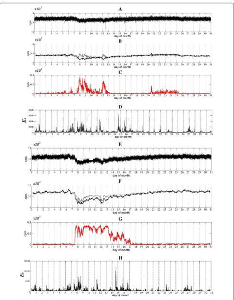
Figure 4 shows the results of neural networks con-structed for Novosibirsk and Athens stations for a period of strong magnetic storms recorded 1 to 31 March 2012. The first storm occurred on 7 to 10 March. The Forbush effect was associated with this storm, which emerged on 8 March, and was expressed in a strong decrease in the level of cosmic rays (up to 10%) at both stations. During the Forbush effect, the absolute values of the network errors significantly increase (up to 10 times), which allowed us to allocate those time periods. A comparison of the geomagnetic data shows that the strongest geo-magnetic disturbances were observed during periods of anomalous behavior of cosmic ray dynamics. During the second magnetic storm (15 to 17 March), the moments of strong increases in the intensity of geomagnetic dis-turbances coincided with the local lowering of the level of cosmic rays and had a more clear manifestation at the Novosibirsk station. Restoration of the level of cosmic rays occurred after the end of the storm.

Experimental results

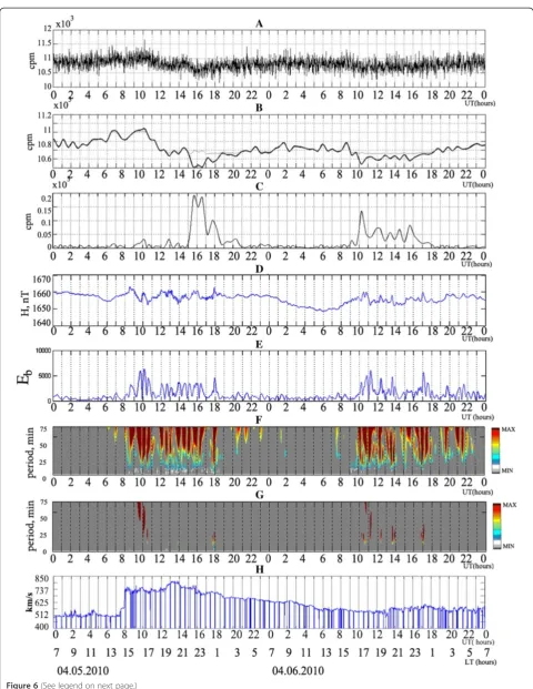
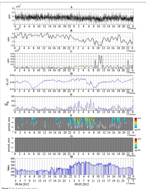
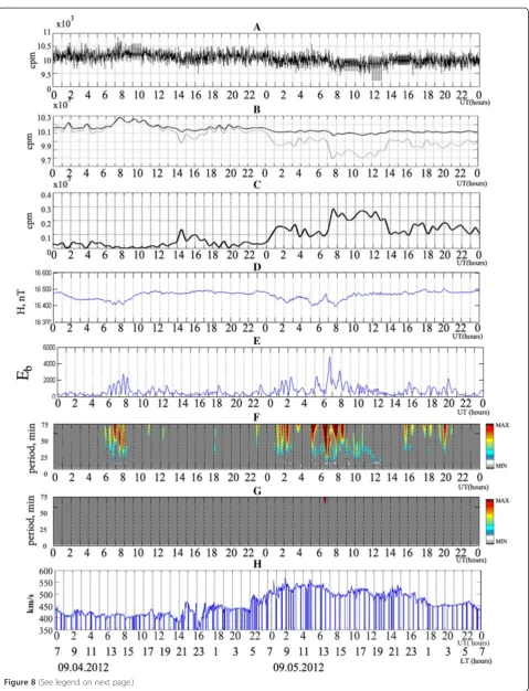
Figures 5 and 6 show the results of the processing of the geomagnetic field and the data of cosmic rays dur-ing magnetic storms that occurred 5 to 7 April 2010. Figures 7 and 8 show the same results but for mag-netic storms that occurred 5 to 6 September 2012.

The first analyzed magnetic storm was registered on Earth on 5 April 2010, at 08.26 UT, as the sudden com-mencement (SC) of the magnetic storm. The speed of the solar wind had increased to 750 to 900 km/s. A globally

observed intense substorm emerged 30 min later in the Earth’s magnetosphere (Kleimenova et al. 2013).

Analysis of Figures 5 and 6 reveals that a local decrease of the level of cosmic rays occurred simultaneously with an increase of geomagnetic disturbance intensity. The error of neural networks increased fourfold at the Athens station and 2.5 times at the Novosibirsk station in com-parison with the quiet period. Decreases in the level of cosmic rays at both stations were accompanied by the most severe disturbances of the geomagnetic field. How-ever, variations of cosmic rays had different behaviors. At the Athens station, a short Forbush effect with rapid re-covery peaked at 20:00 UT, in which the neural network error increased in threefold in comparison with the quiet period. At the Novosibirsk station, the Forbush effect was longer and peaked at 16:00 UT; the neural net-work error increased tenfold in comparison with the quiet period. The intensity of the geomagnetic field disturbances reached maximum values during 9:26 to 10:07 UT.

The second analyzed magnetic storm was recorded on Earth on 5 September 2012. The polar wind velocity reached values of 500 to 600 km/s due to the arrival of the accelerated flow from the coronal mass ejection (CME) that occurred on 2 September 2012. Detailed analysis of Figures 7 and 8 reveals that local increases in intensity of geomagnetic disturbances emerged at the analyzed stations in different frequency ranges and that periods of weak geomagnetic activity had been formed on the eve of storm (approximately 06:00 to 08:00 UT, 10:30 to 12:30 UT, and 17:00 to 18: 00 UT on 4 September and from 22:00 UT until the start of the storm). The arrival of the shock wave occurred at 1:00 UT on 5 September, and both stations simultan-eously recorded the beginning of the Forbush effect; an increase in the error of the neural network was recorded at the Novosibirsk station. Maximal values of intensity field disturbances were recorded on 5 September during 6:43 to 6:48 UT, which coincides with the periods of strong geomagnetic activity. At the Novosibirsk station, the maximum of the lowering of the level of cosmic rays and neural network error had increased in ten times in comparison with the quiet period. It should be noted that the Forbush effect registered at the Athens station was short, and the cosmic ray level recovered fast, whereas the Forbush effect registered at Novosibirsk station was more extended.

(16)

Conclusions

We proposed a model of geomagnetic field variations that allows us to describe the tranquil dynamics and disturbances occurring in periods of increased geomag-netic activity. On the basis of this model, we developed methods for assessing changes in energy characteristics of the field and allocation of periods of weak and strong geomagnetic activity. The analysis showed that in pe-riods of increased geomagnetic activity, the developed tools allowed us to record the onset of geomagnetic dis-turbances and to receive quantitative estimates of the power of the geomagnetic field disturbance. Such appli-cations allowed us to perform detailed analysis of geo-magnetic field variations for different registration stations during strong magnetic storms.

A slight increase in geomagnetic activity, which is as-sociated with the approaching storm, was observed in different frequency ranges at local moments on the eves of storms.

Moreover, we proposed methods of approximation of the time variation of cosmic ray data and allocation of anomalous changes occurring during periods of high solar activity. The methods for Novosibirsk, Athens, Cape Schmidt, and Apatity stations were built in neural networks that approximate the time variation in the smoothed component of the cosmic rays. In the training of the networks, we used data recorded in 2005 to 2013. This method allowed us to study the structure of the data of cosmic rays in detail and to allocate abnormal changes in their dynamics during periods of the Forbush effects.

Joint analysis of the data of the geomagnetic field and cosmic rays in the periods of strong magnetic storms showed that the strongest geomagnetic field perturba-tions were observed in periods of anomalous changes in the dynamics of cosmic rays and could be registered on the basis of the proposed applications.

Future plans include adaptation of the developed tools for a larger number of registration stations and creation of an integrated software environment that would pro-vide the possibility of spatio-temporal data analysis in an online mode.

Competing interests

The authors declare that they have no competing interests.

Authors’contributions

OVM proposed a method for describing variations of the geomagnetic field based on wavelets and an approach to solving the problem of data approximation of the cosmic rays based on a combination of multiresolution wavelet decompositions with neural networks. ISS proposed the computing solutions for estimating changes in the energy characteristics of the field and the allocation of periods of increased geomagnetic activity in addition to algorithms for processing and analysis of geomagnetic data. TLZ developed a method for approximating the time variation of cosmic rays and allocation of abnormal changes in their dynamics based on multiresolution wavelet decompositions and neural networks in addition to algorithms for processing and analysis of the data of cosmic rays. All authors read and approved the final manuscript.

Acknowledgements

This research is supported by a grant of Russian Academic Fund No. 14-11-00194. We thank researchers of the NMDB project (www.nmdb.eu/) for providing high-resolution neutron monitor data and those at Intermagnet (www.intermagnet.org) for promoting high standards of magnetic observatory practices.

Author details

1

Institute of Cosmophysical Researches and Radio Wave Propagation, Mirnaya Str., 7, Kamchatka Region, Elizovskiy District, Paratunka 684034, Russia.2Kamchatka State Technical University, Klyuchevskaya Street 35, 683003 Petropavlovsk-Kamchatsky, Russia.3_{Saint Petersburg Electrotechnical} University“LETI”, Ulitsa Professora Popova, 5, St Petersburg, Russia.

Received: 31 March 2014 Accepted: 29 October 2014

References

Akasofu SI, Chapman S (1972) Solar-terrestrial physics. Oxford University Press, Oxford Bartels J, Heck NH, Johnston HF (1939) The three hour range index measuring

geomagnetic activity. J Geophys Res 44:411–454

Bishop CM (1995) Neural networks for pattern recognition. Oxford University Press Inc., New York

Chui CK (1992) An introduction in wavelets. Academic Press, New York Daubechies I (1992) Ten lectures on wavelets. CBMS_–NSF lecture notes nr. 61.

SIAM, Philadelphia

Hafez AG, Ghamry E, Yayama H, Yumoto K (2013) Systematic examination of the geomagnetic storm sudden commencement using multi resolution analysis. Adv Space Res 51:39–49

Haykin S (1999) Neural networks: a comprehensive foundation, 2nd edn. Prentice-Hall, New York

Ivanov VV, Rotanova NM, Kovalevskaya EV (2001) The wavelet analysis as applied to the study of geomagnetic disturbances. Geomagn Aeron 41:583–591

Jach A, Kokoszka P, Sojka J, Zhu L (2006) Wavelet-based index of magnetic storm activity. J Geophys Res 111:A09215, doi:10.1029/2006JA011635

Kleimenova NG, Zelinskii NR, Kozyreva OV, Malysheva LM, Solov’ev AA, Bogoutdinov SR (2013) Pc3 geomagnetic pulsations at near-equatorial latitudes at the initial phase of the magnetic storm of April 5, 2010. Geomagn Aeron 53:313–320

Kóta J, Somogyi A (1969) Some problems of investigating periodicities of cosmic rays. Acta Physica Acad Sci Hung 27:523_–548

Kozlov VI, Markov VV (2007) Wavelet image of a heliospheric storm in cosmic rays. Geomagn Aeron 47:52–61

Kudela K, Yasue S, Munakata K, Bobik P (1999) Cosmic ray variability at different scales: a wavelet approach. Proceedings of the 26th International Cosmic Ray Conference, Salt Lake City, USA

Levin BR (1963) Theoretical basis of statistical radio techniques. Fizmatgiz, Moscow Lundstedt H, Liszka L, Lundin R (2005) Solar activity explored with new wavelet

methods. Ann Geophys 23:1505_–1511, doi:10.5194/angeo-23-1505-2005 Macpherson KP, Conway AJ, Brown JC (2001) Prediction of solar and geomagnetic

activity data using neural networks. J Geophys Res 100:735–744

Mallat S (1999) A wavelet tour of signal processing. Academic Press, London Mandrikova OV, Solovev IS (2013) The method of the extracting disturbance and

estimates of the Earth’s magnetic field is based on the wavelet-packet. Proceedings of 11th International Conference on Pattern Recognition and Image Analysis, Samara, Russia

Mandrikova OV, Solovjev I, Geppenerc V, Taha A-KR, Klionskiy D (2013) Analysis of the Earth’s magnetic field variations on the basis of a wavelet-based approach. Digit Signal Process 23:329_–339

Nayar SRP, Radhika VN, Seena PT (2006) Investigation of substorms during geomagnetic storms using wavelet techniques. Proceedings of the ILWS Workshop Goa, India

Paschalis P, Sarlanis C, Mavromichalaki H (2013) Artificial neural network approach of cosmic ray primary data processing. Sol Phys 182(1):303_–318

Rotanova N, Bondar T, Ivanov V (2004) Wavelet analysis of secular geomagnetic variations. Geomagn Aeron 44:252–258

Rybàk J, Antalovà A, Storini M (2001) The wavelet analysis of the solar and cosmic-ray data. Space Sci Rev 97:359–362

Segarra A, Curto JJ (2013) Automatic detection of sudden commencements using neural networks. Earth Planets Space 65(7):791–797

(17)

Soloviev A, Chulliat A, Bogoutdinov S, Gvishiani A, Agayan S, Peltier A, Heumez B (2012) Automated recognition of spikes in 1 Hz data recorded at the Easter Island magnetic observatory. Earth Planets Space 64(9):743–752

Vecchio A, Laurenza M, Storini M, Carbone V (2012) New insights on cosmic ray modulation through a joint use of nonstationary data-processing methods. Adv Astronomy 2012. doi:10.1155/2012/834247

Woolley JW, Agarwarl PK, Baker J (2010) Modeling and prediction of chaotic systems with artificial neural networks. Int J Numer Methods Fluids 63, doi:10.1002/fld.2117

Xu Z, Zhu L, Sojka J, Kokoszka P, Jach A (2008) An assessment study of the wavelet-based index of magnetic storm activity (WISA) and its comparison to the Dst index. J Atmos Solar Terr Phys 70:1579–1588

Zaourar N, Hamoudi M, Mandea M, Balasis G, Holschneider M (2013) Wavelet-based multiscale analysis of geomagnetic disturbance. Earth Planets Space 65(12):1525–1540

doi:10.1186/s40623-014-0148-0

Cite this article as:Mandrikovaet al.:Methods of analysis of geomagnetic field variations and cosmic ray data.Earth, Planets and Space201466:148.

Submit your manuscript to a

journal and beneﬁ t from:

7 Convenient online submission 7 Rigorous peer review

7 Immediate publication on acceptance 7 Open access: articles freely available online 7 High visibility within the ﬁ eld

7 Retaining the copyright to your article