R E S E A R C H
Open Access
Fast compression of OFDM channel
state information with constant frequency
sinusoidal approximation
Avishek Mukherjee and Zhenghao Zhang
*Abstract
We propose CSIApx, a very fast and lightweight method to compress the channel state information (CSI) of Wi-Fi networks. CSIApx approximates the CSI vector as the linear combination of a small number of base sinusoids on constant frequencies and uses the complex coefficients of the base sinusoids as the compressed CSI. While it is well-known that the CSI vector can be represented as the linear combination of sinusoids, fixing the frequencies of the sinusoids is the key novelty of CSIApx, which is guided by our mathematical finding that almost any sinusoid can be approximated by a set of base sinusoids on constant frequencies. CSIApx enjoys very low computation complexity, because key steps in the compression can be pre-computed due to the constant frequencies of the base sinusoids. We extensively test CSIApx with both experimental and synthesized Wi-Fi channel data, and the results confirm that CSIApx can achieve very good compression ratio with little loss of accuracy.
Keywords: Channel state information, Compression, Approximation
1 Introduction
In Wi-Fi, the channel state information (CSI) for an antenna pair is a vector of complex numbers, represent-ing the channel coefficients of the orthogonal frequency division multiplexing (OFDM) subcarriers. The CSI is needed to calculate the modulation parameters for tech-niques such as multi-user multiple-input-multiple-output (MU-MIMO). In Wi-Fi, the CSI is typically measured at the receiver and is transmitted back to the sender, which requires significant overhead. For example, on a 20-MHz channel with 64 subcarriers, the full CSI for a single antenna pair has 64 complex numbers, and for 9 antenna pairs, 576. Although Wi-Fi does not use all subcarriers, the feedback for 9 antenna pairs still may exceed 1000 bytes. The Wi-Fi standard [1] defines options to compress the CSI, such as reducing the quantization accuracy or the number of subcarriers in the feedback or using the Given’s rotation on the V matrix after the singular value decomposition (SVD) of the CSI matrix. However, these methods either reduce the accuracy of the CSI or only achieve modest compression ratios. For example, a 3 by
*Correspondence:[email protected]
Department of Computer Science, Florida State University, Tallahassee, FL, USA
3 complex V matrix can only be compressed into 6 real numbers, at a compression ratio of 3.
In this paper, we propose CSIApx, a novel CSI compres-sion method for Wi-Fi networks with the following key features: (a)high compression ratio, e.g., capable of com-pressing the CSI of 40 subcarriers in most of our Wi-Fi experiments into just 6 or less complex numbers; (b)little loss of accuracy, e.g., the decompressed CSI is very close to the measured CSI; and (c)very low computation complex-ity, suitable for hardware implementation. Compared to the Givens rotation, CSIApx achieves higher compression ratio, e.g., more than 2.5 times higher with our experi-mental data. Compared to other recent solutions in the literature [2–4], CSIApx has much lower computation complexity, because its main computation is simply the dot products between the CSI and a small number of constant vectors.
CSIApx is based on the well-known fact that the CSI is the linear combination of sinusoids [3,4], where each sinusoid is the result of a physical path in the channel. Previous approaches solve complex optimization prob-lems to find the parameters of the physical paths, i.e., the frequencies, the phases, and the amplitudes of the sinusoids. Radically different from such solutions, CSIApx
does not attempt to find the parameters of the physi-cal paths. Instead, CSIApx uses the linear combination of a set of base sinusoids, which are on fixed frequen-cies, to approximatethe CSI, and our results show that the approximation usually achieves very high accuracy. This approach is guided by our mathematical finding that the linear combination of sinusoids on constant frequen-cies can approximate any given sinusoid very well, which is explained in more details in Section3. Roughly speaking, as each individual sinusoid can be approximated by just a small number of base sinusoids, the entire CSI, which is the summation of the individual sinusoids, can also be approximated,regardless of the number and characteris-tics of actual paths in the channel. Working with base sinu-soids on fixed frequencies has two major benefits. First, it avoids solving complex optimization problems and dra-matically reduces the computation complexity. Second, as the frequency values of the base sinusoids are constants, they do not need to be transmitted, further improving the compression ratio. While CSIApx is primarily designed for compressing the CSI of Wi-Fi channels, it will theo-retically work on any OFDM-based system that measures the channel state information, as long as the delay spread is not too large.
The rest of the paper is organized as follows. Section2
discusses related work. Section 3 explains the theoreti-cal foundations. Section 4 describes CSIApx. Section 5
describes the evaluation. Section6concludes the paper.
2 Related work
CSI compression has been a major topic of interest due to its practical importance in wireless networks. The differ-ences between CSIApx and the existing methods in Wi-Fi have been discussed in Section1. Some early approaches [5–7] use quantization and general purpose compression techniques like the Huffman coding, with typical com-pression ratios around 3:1, lower than that with CSIApx. Another popular approach is to reduce the frequency or the amount of CSI feedback in slow-varying channels sim-ilar to those in [8, 9], which complements compression techniques such as CSIApx. AFC [10] chooses from exist-ing compression options for the least degradation of link throughput, which can be complemented by CSIApx as an additional compression option. The problem of consoli-dating CSI from a small number of settings to predict the CSI under other settings has been studied in [11], which is different from CSI compression.
Sparsity in certain wireless channels has been well-known [3,4,12–14] and has been exploited in applications such as CSI compression and CSI estimation. Unlike exist-ing work that usually still attempts to find the actual paths by solving optimization problems, CSIApx focuses on approximatingthe CSI withconstantfrequency sinusoids, which leads to much lower computation complexity than
the existing algorithms such as CTDP [3,4]. CSIApx also has much lower complexity than CSIFit [2], which uses the Levenberg-Marquardt (LM) algorithm to compress the CSI of MIMO channels, because the LM algorithm needs to solve a set of linear equations in each itera-tion. R2-F2 [15] uses the CSI measured on one direction of the wireless link to predict that of the other, which requires much more computation than CSIApx; in addi-tion, R2-F2 depends on channel reciprocity, which may not be true depending on the hardware circuitry, and may also need periodical calibrations [16], which is why Wi-Fi defines explicit CSI feedback and does not solely depend on channel reciprocity to obtain the CSI.
We have presented an initial version of CSIApx in [17] and have obtained a patent [18]. Compared to the con-ference version, this paper contains significant improve-ments in the theoretical foundation and the compression ratio in practice.
3 Theoretical foundation
We prove that a target sinusoid on frequency g can be approximated as the linear combination of P base sinu-soids and the approximation error decays exponentially fast as the number of base sinusoids increases, where the frequencies of the base sinusoids are constants. Therefore, the summation of many sinusoids, such as the CSI vector, can still be approximated as the linear combination of only Pbase sinusoids.
3.1 Approximating real sinusoids
We begin with a theorem on the approximation of real sinusoids.
Theorem 1 Consider P base sinusoids on evenly spaced frequencies:{cos(0x), cos(δx), ..., cos[(P−1)δx]}. Suppose cos(gx)is to be approximated as the linear combination of the base sinusoids for x∈[ 0,X], where0≤g≤(P−1)δ. If Xδ <1, there exists an approximation with error decaying exponentially fast as P increases.
G()is infinitely differentiable, the Lagrange interpolation and we claim that
Clearly, ifXδ <1, the interpolation error decays exponen-tially fast asPincreases. Finally, note that the argument is true for any point in [ 0,X].
3.2 Extensions
We now discuss a few extensions.
Extension to sin(gx) : With exactly the same argu-ments, it can be proved that sin(gx) can be approxi-mated as the linear combination of the base sinusoids. Clearly, for the approximation of sin(gx), exactly the same coefficients as the coefficients for the approxima-tion of cos(gx) can be used, because the coefficients are determined only by g and the frequencies of the base sinusoids.
Extension to [−X, X] : The extension to [−X,X] is immediate. That is, if the approximation matches cos(gx) in [ 0,X], multiplying the base sinusoids by the same coef-ficients for x in [−X, 0] should also result in a match, because the target sinusoid and the base sinusoids have the same parity.
Extension to eigx:The extension to complex waveeigxis clearly
3.3 The summation of many sinusoids
So far, we considered approximating one target sinu-soid. The CSI vector, on the other hand, may be the
summation of many sinusoids. However, if the base sinu-soids are selected correctly, any individual sinusoid in the CSI vector can be approximated, and therefore, the summation can also be approximated with the same set of base sinusoids. The deterministic maximum approx-imation error will be the summation of all individual approximation errors and may be large. However, in prac-tice, the sinusoids in the CSI have random phases and the errors almost never add up constructively. A prob-abilistic bound therefore is more suitable; however, it depends on the assumptions of the path delay and power distribution. We instead choose to use both the real-world data and synthesized data to evaluate CSIApx and the results show that CSIApx approximates the CSI very well.
4 CSIApx
CSIApx is a fast compression method based on our theo-retical findings. We begin with an overview.
4.1 Overview
According to our theoretical findings, the CSI can be approximated as the linear combination of the base sinu-soids. The coefficients of the base sinusoids in the lin-ear combination can be found by minimizing the fit residual, defined as the total squared error between the CSI vector and the approximation. The approximation is therefore called an MSE Fit and requires very low computation complexity, mainly because the linear sys-tem to be solved in the optimization problem is defined by a constant matrix. As any sinusoid can be approxi-mated in this manner, the simplest approach would be to select just one set of base sinusoids to be used for all CSI. However, different types of channels have dif-ferent delay spreads, which translate to difdif-ferent fre-quency ranges of the sinusoids in the CSI, the larger the delay spread, the higher the frequency. As sinu-soids on lower frequencies can be approximated with fewer base sinusoids, to further improve the compression ratio, a small number ofconfigurationsare used in CSI-Apx which have different orders, where the order refers to the number of the base sinusoids. CSIApx finds the MSE Fit coefficients for all configurations and selects a configuration, considering both the compression ratio and the fit residual. The computation complexity is also reduced by sharing certain base sinusoids among multiple configurations.
4.2 The MSE Fit
4.2.1 Finding the MSE Fit
The core of CSIApx is to find the coefficients of the MSE Fit, denoted as a vector.
J=
wherePis the order;γkandfkare the coefficient and fre-quency of base sinusoidk, respectively;yjis elementjin the CSI vectorY; andNis the length of the CSI vector. By taking the derivatives ofJwith respect to the coefficients and setting them to 0,that minimizesJis the solution to a linear systemQ=S, where:
• Qis aPbyPmatrix, in whichqk,h=jN=1ei(fh−fk)j,
• Sis aPby 1 vector, in whichsk =jN=1e−ifkjyj. It can be seen thatSis determined by the CSI vector, but is just the dot products of the CSI vector and the conjugate of the base sinusoids. On the other hand, as the frequency values are constants, Q−1 is a constant matrix and can be pre-computed. Therefore, after S is obtained, can be found by simply multiplying the constant matrixQ−1 withS.
4.3 The compression process of CSIApx
CSIApx hasUconfigurations. Configurationuis defined by the frequencies of itsPubase sinusoids, denoted asfu,k fork = 1, 2, ...,Pu, where the frequency is the amount of angular rotation between neighboring points in the CSI vector. For each configuration, CSIApx solves the constant linear system in Section 4 to get the coefficients of the MSE Fit. To evaluate the quality of the fits, for each config-uration, CSIApx evaluates the MSE Fit onLevenly spaced sample points, whereL= N4, and finds the total fit resid-ual on the sampled points, denoted asηufor configuration u. The MSE Fit is not evaluated on all points to reduce the computation complexity. CSIApx selects the fit coeffi-cients of configurationuas the compressed CSI, ifuis the smallest index satisfyingηu < ζmin{η1,η2, ...,ηU}, where
ζ is a constant, empirically chosen as 1.75 and 4 for CSI with 64 and 40 subcarriers, respectively.
4.4 The configurations and the base sinusoids
The configurations and base sinusoids should be selected considering compression ratio, accuracy, implementation cost, and the range of the fit coefficients. As Wi-Fi has a fixed number of subcarriers and well-studied types of channels [19], we select a configuration for each type of channel.
4.4.1 Finding parameters for a given channel type
For a given type of channel, the parameters to be deter-mined include the number of base sinusoids, denoted here asP, and the frequencies of each base sinusoid, denoted here asf1,f2, ...,fP. Note thatf1is actually always 0 to be able to cover the lowest frequency. Our approach is to first solve the problem of determining the frequencies of the
base sinusoids for a givenP, then conduct a linear scan on Pto find the bestP. As the linear scan is straightforward, in the following, we focus on the first problem.
As a channel has multiple paths, while paths of differ-ent delays may not have equal power, the selection of the base sinusoids will have to be based on the power profile of the channel. For example, if 90% of the power is con-centrated within a certain small delay range, more base sinusoids should be allocated to the corresponding range of frequencies. The power profile is generated using the delay taps and relative power values for the given chan-nel model. It also takes into account possible imperfect symbol-level synchronization, which is assumed to be uni-formly within 0 to 50 ns, because such synchronization error will increase the frequencies of the sinusoids.
The problem of finding the base sinusoid frequencies for givenPis solved using a standard solver like Levenberg-Marquardt. First, from 0 to the maximum frequency in the power profile,H evenly spaced frequencies are selected, denoted asg1togH. The objective function passed to the solver basically minimizes the total fit residual of all sinu-soid on such frequencies, which are weighted according to the power profile. By doing so, the solver should find a set of base sinusoids that is expected to minimize the fit residual of this type of channel. To be more specific, the objective function is defined as follows withf2,f3, ...,fP as soid of frequencygs when the base sinusoid frequencies are 0,f2,f3, ...,fP, andW(gs)is the power profile weight of frequencygs. It should be noted that some noise is added to the pure sinusoids such that the signal-to-noise ratio (SNR) is 20 dB, to emulate a real-world scenario.
4.4.2 Results
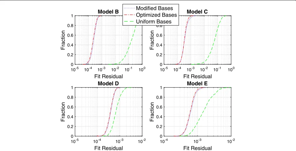
Figure1shows, in log scale, the output of the solver for dif-ferent numbers of base sinusoids of Wi-Fi channel model B to E, when the number of subcarriers is 64. It can be seen that the fit residual decreases exponentially as the number of bases increases up to a point, after which there is very little change to the final fit residual. In fact in some cases, the fit residual increases slightly with more bases. This is due to over-fitting, i.e., the MSE Fit trying to follow the noise in the data. Based on this result, the selected num-bers of bases for each configuration are 5, 7, 11, and 17, respectively.
4.4.3 Manual tuning
1 3 5 7 9 11 13 15 17 19
Fig. 1Results of the base selection process. The output of the solver
is shown for different numbers of base sinusoids of Wi-Fi channel model B to E, when the number of subcarriers is 64
channel with a single path, which we have covered with an additional simple configuration with three base sinu-soids. Channel model F is excluded because it requires a large number of base sinusoids to approximate and as such does not bring in much in terms of compression. More-over, based on our experience, model F rarely occurs in indoor Wi-Fi networks.
Figure2shows, in log scale, a comparison of the cumu-lative density function (CDF) of the fit residual per point when running MSE Fit using these optimized base soids as opposed to using uniformly spaced base sinu-soids. These tests were performed on 1000 CSI vectors with 20-dB SNR for each channel model. It can be seen that the optimized base sinusoids often resulted in an
order of magnitude or greater reduction in the approxi-mation error.
We note that the main computation cost in CSIApx is actually finding the dot products between the base sinusoids and the CSI. If a base sinusoid used in one con-figuration can be used by another, the computation cost can be reduced.
Therefore, we slightly modified the optimized base sinu-soid frequencies, to allow one base sinusinu-soid to be used for more than one configuration when possible. For 64 subcarriers, the selected base frequencies for the five con-figurations are {0, 0.06, 0.12}, {0, 0.05, 0.1, 0.15, 0.25}, {0, 0.06, 0.12, 0.18, 0.24, 0.3, 0.42}, {0, 0.06, 0.12, 0.18, 0.24, 0.3, 0.36, 0.42, 0.525, 0.6375, 0.75}, and {0, 0.075, 0.15, 0.225, 0.3, 0.375, 0.45, 0.525, 0.6, 0.7, 0.8, 0.9, 1.0, 1.1, 1.2, 1.3}, respectively. In total, there are 27 unique base sinusoids. Figure1also shows the CDF of the fit residual when running MSE Fit with this modified set of base sinu-soids. It can be seen that there is a small difference under 10% when compared against the optimized base frequen-cies. However, these modified configurations cut down the complexity of CSIApx considerably. It should also be noted that for channel model E, the number of base sinu-soids was reduced from 17 to 16, as there is very little loss in accuracy at 20 dB, but leads to a higher compression ratio.
We repeated the same process also for CSI vectors of 40 subcarriers, which is used in our experiments. The five configurations are {0, 0.05, 0.10}, {0, 0.06, 0.12, 0.2},
10-5 10-4 10-3 10-2 10-1 100
Fig. 2Fit residual as a function of the number of base sinusoids. A comparison of the cumulative density function (CDF) of the fit residual per point
{0, 0.075, 0.15, 0.225, 0.3, 0.45}, {0, 0.075, 0.15, 0.225, 0.3, 0.375, 0.525, 0.675, 0.825, 0.975}, and {0, 0.09, 0.18, 0.27, 0.36, 0.45, 0.575, 0.7, 0.825, 0.95, 1.075, 1.2, 1.325, 1.45}, respectively. In total, there are 27 unique base sinusoids.
4.5 Complexity of CSIApx
Overall, letW be the total number of unique base sinu-soids in all configurations; the complexity of CSIApx, measured by the number of complex multiplications, includes only:
• WN: for computing the dot products between the base sinusoids and the CSI
• U
u=1P2u: for finding the fit coefficients of all configurations
• U
u=1(Pu+1)L: for computing the fits at sampled points and the sampled fit residuals
4.6 Coping with shift frequency
In practice, the raw measured CSI often has a shift fre-quency, which is a frequency value added to the frequen-cies of all sinusoids, caused by the sample timing offset to the OFDM symbol boundary. The shift frequency needs to be removed before running CSIApx, because it may force CSIApx to choose higher configurations to approximate sinusoids on higher frequencies and reduce the compres-sion ratio. This can easily be achieved by multiplying the CSI with a sinusoid on the negative of the shift frequency, a process we callrotation. The value of the shift frequency is known to the wireless receiver, because it selects the OFDM symbol boundary. The frequency used in the rota-tion can also be slightly adjusted to make sure that the sinusoids in the CSI are still on positive frequencies after the rotation.
5 Results and discussion
We report our evaluation of CSIApx on both real-world and synthesized CSI data in this section.
5.1 Evaluation with the experimental CSI data
We first discuss our evaluation of CSIApx with the real-world experimental CSI data.
5.1.1 Data collection and preprocessing
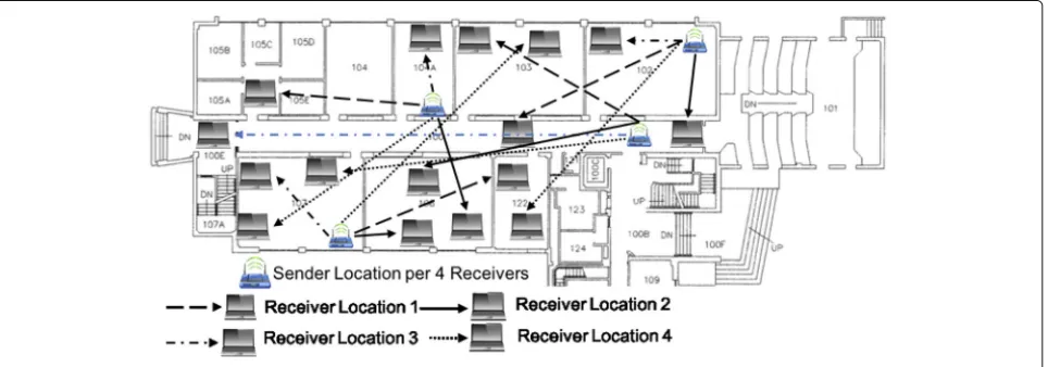
CSI data was collected using the Atheros CSITool [20] installed on two laptops with the Atheros AR9462 wire-less card with two antennas on 20-MHz channels. A total of 100 experiments in various location settings were con-ducted, which include typical environments like office buildings, apartment complexes, and large hallways. The experiments include both line of sight and non-line of sight cases as well as varying channel conditions due to human movements near the machines. Some of the experiment locations are shown in Fig.3.
The CSITool reports the CSI on 56 selected subcarriers for four antenna pairs. Figure4shows the absolute values of some raw CSI vectors, where it can be seen that the data has some level of noise. A few preprocessing steps were taken before passing the data for compression. Firstly, as the signal always seems to be attenuated at both ends of the spectrum, caused most likely by additional filtering in hardware, not representing the characteristics of the actual channel, 8 subcarriers on both ends are removed, with only the middle 40 subcarriers kept. Secondly, as some of the experiments have very weak signals, measure-ments with RSSI lower than 30 dB were not used. Thirdly, the CSI data of all antenna pairs is normalized by a com-mon factor such that the maximum amplitude is 1. Lastly, as explained before, each CSI vector is rotated to remove the shift frequency. As the shift frequency value is not reported by our current device to the driver level, a simple estimation method is used, which basically keeps rotating the CSI from the same transmitting antenna incremen-tally, until most energy appears to occupy only a spectrum starting from 0 up to some frequency for both receiving antennas. As it may over-rotate the CSI and lead to neg-ative frequencies, when running CSIApx, the CSI for all
Subcarriers
0
-30 -20 -10 0 10 20 30
0.1 0.2 0.3 0.4 0.5 0.6 0.7 0.8 0.9 1
Amplitude
Exp1 Exp2 Exp3 Exp4
Fig. 4Absolute values of some measured CSI. The absolute value of the CSI across 64 subcarriers is shown for the strongest antenna pair in four
experiments
antenna pairs are multiplied by a sinusoid with a positive frequency of 0.0491 to move most sinusoids in the CSI to positive frequency.
5.1.2 Compared methods
For comparison, we also implement the CTDP extraction algorithm according to [4], referred to as CTDP, which iteratively selects a sinusoid that best matches the current residual signal, until the power of the selected sinusoid is below a threshold. CTDP is chosen because it is one of the more recent methods and has a good performance. As CTDP requires the noise power value, which needs to be estimated with the experimental data, we use the fit residual found by CSIApx as the total noise power, which should be very close. The frequency range of sinusoids scanned in CTDP is [−0.785, 1.57], which should cover all frequencies in the CSI. Another constrained version of CTDP, referred to as cCTDP, is also evaluated, with which the fit residuals of CTDP and CSIApx can be com-pared when using similar number of sinusoids. That is, with cCTDP, the number of sinusoids used is the small-est upper bound of the average number of sinusoids used by CSIApx for the same CSI measurement, noting that CSIApx may use different configurations for the differ-ent antenna pairs. It should also be mdiffer-entioned that as CTDP has to solve an optimization problem to select the frequency of a sinusoid in each iteration, it has much higher implementation complexity than CSIApx, because CSIApx avoids this problem altogether by using constant frequencies.
Two other methods were also implemented, but the results are not shown in the figures in this section, since their performances are not comparable with CSIApx and CTDP. One of the methods is CSIFit [2], the median of fit residual of which, for example, is more than six times
than that with CSIApx for the experimental data, while the compression ratio is about the same. The other maybe obvious approach, i.e., keeping only a small number of sig-nificant FFT coefficients, is also not included, because it usually has an order of magnitude higher fit residual than CSIApx even when using twice number of coefficients.
5.1.3 Fit accuracy and compression ratio
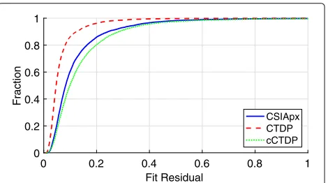
As the fit residual and the compression ratio are related, i.e., improving one is often at the cost of the other, they are jointly compared. Figure5shows the CDF of the total fit residual of all four antenna pairs in 7923 CSI measure-ments. Figure6shows the compression ratio, which is the number of real numbers in the CSI vector divided by that needed by a compression method to describe the sinu-soids, noting that a complex number consists of two real numbers.
0 0.2 0.4 0.6 0.8 1
Fit Residual 0
0.2 0.4 0.6 0.8 1
Fraction
CSIApx CTDP cCTDP
Fig. 5Fit residual with experimental data. A comparison of the
2 4 6 8 10 12
Fig. 6Compression ratio with experimental data. A comparison of
the cumulative density function (CDF) of the compression ratio achieved when running CSIAPx versus CTDP versus CCTDP
It can be seen that the fit residual of CSIApx in most cases are very small with a median of 0.0828 for all antenna pairs, which translates to an error of 0.0005 per data point. The fit residual of CTDP is better with a median of 0.0467, however it is at a cost of a much lower compression ratio, as the average compression ratio of CSIApx against 40 subcarriers is 7.68, much better than CTDP, which is 3.59. By closely examining the fits, we found that CSIApx actually fits the signal very well, and its fit residual is mainly the quantization noise, such as those shown in Fig.4, which cannot be eliminated unless more sinusoids are introduced to fit the noise. In this sense, CSI-Apx achieves a better tradeoff between fit residual and compression. The better performance with CSIApx can also be seen from the cCTDP results, as cCTDP actu-ally has higher fit residual, at the same time slightly lower compression ratio.
5.1.4 MU-MIMO rate
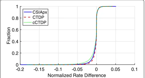
The end result of the compression method can be the MU-MIMO data rate of the users. We use the MU-MIMO rate program at [21], which first calculates the modulation parameters with the supplied imperfect CSI, then finds the achievable data rate when the selected parameters are used on the actual channel. We configure the program to use the greedy method for user selection and run at SNR of 20 dB. For each subcarrier, we run the program twice, feeding the compressed and the measured CSI to the pro-gram to obtain two values, representing total data rates to all users with imperfect and perfect CSI, respectively. The difference between the two, divided by the latter, is called thenormalized rate differenceand is used as the metric.
A total of 1500 tests are run, where each test has one sender and two receivers. In each test, we use the CSI collected from experiments where the sender was at a fixed location for four receivers, and randomly select two receivers from the four actual receivers. As the link is 2 by 2 but each MU-MIMO receiver has only one antenna, we
select the first antenna for each receiver. Figure7 shows the CDF of the normalized rate difference, where we can see that the rate difference with CSIApx is usually very small, e.g., within−3% and 3% in over 98.3% of the cases. CTDP performs better reporting 99.0%, but this comes at the cost of its compression ratio. At similar compression ratio, cCTDP performs worse than CSIApx at 95.7%. The rate difference in some very rare cases can also be positive, since the greedy method sometimes selects different sets of users when given the compressed and measured CSI.
5.1.5 Parameter distribution
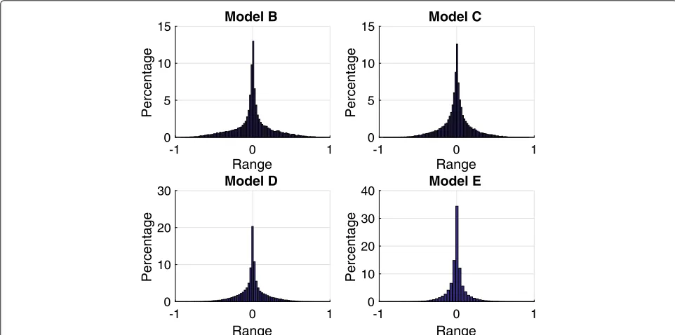
One of the nice features of CSIApx is that the fit coeffi-cients stay in a small range, making it simple and inex-pensive to quantize and transmit the coefficients as the compressed CSI. Figure8 shows the distribution of the real and imaginary parts of the coefficients found by CSI-Apx for the strongest antenna pair in each test case, because the distributions for other antenna pairs should just be its scaled versions. We can see that all numbers resides in a small range with smooth density.
5.2 Evaluation with synthesized CSI data
We test CSIApx with synthesized CSI data, which comple-ments the experimental evaluation by challenging CSIApx with more channel types and testing CSIApx under con-trollable settings like the SNR level.
5.2.1 CSI generation
We use the channel model code at [19] to generate CSI for all 64 subcarriers in Wi-Fi on 20-MHz chan-nels for 3 by 3 links with nine antenna pairs. Four cases, referred to as model B, model C, model D, and model E, are used, which represent typical indoor environments with around 100-ns, 200-ns, 400-ns, and 800-ns delay spread, respectively, and should cover the majority of typ-ical Wi-Fi channels. The maximum amplitude is again normalized to 1. White Gaussian noise is added to the
-0.2 -0.15 -0.1 -0.05 0 0.05 0.1 Normalized Rate Difference
0
Fig. 7Normalized rate difference with experimental data. A
-3 -2 -1 0 1 2 3 Value
0 5 10 15 20
Percentage
Fig. 8Coefficient values with experimental data. The distribution of
the real and imaginary parts of the coefficients found by CSIApx is shown for the strongest antenna pair in the each experimental test case
CSI vector, and a total of 1000 test cases are performed for each SNR level. To simulate imperfect rotation, the CSI is further multiplied by a sinusoid with random fre-quency, which translates to within 0 to 50 ns of timing error.
5.2.2 Fit accuracy and compression ratio
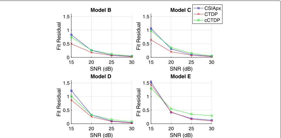
As the clean CSI is available, when calculating the final fit residual, the fit is compared with the clean CSI; all prior steps are still based on the noisy CSI. Figure9shows the mean of the total fit residual of all antenna pairs in various settings. The fit residual of CSIApx is usually very small,
such as about 0.0007 or lower per point at 20 dB or above. In addition, as the noise level reduces by 5 dB, the fit resid-ual in most cases also reduces by roughly 5 dB, suggesting that the fit residual is mostly noise. Figure10shows the average compression ratios. It can be seen that CSIApx achieves very high compression ratios in many cases, i.e., above 12.4:1, 7.9:1, 5.5:1, and 4.0:1 against 64 subcarriers for models B, C, D, E, respectively, when the SNR is 20 dB or above. More complicated channel conditions do pose a challenge to CSIApx as it has to use higher configurations. Also, although CSIApx may have slightly larger fit resid-ual, it has much higher compression ratios than CTDP in all cases. In addition, the compression ratio CSIApx is more stable than CTDP for each model when the SNR is 20 dB or higher, suggesting the CSIApx is better at captur-ing the actual signal and less susceptible to the influence of noise. cCTDP has higher fit residual and lower compres-sion ratios in almost all cases when the SNR is 20 dB or higher.
5.2.3 MU-MIMO rate
MU-MIMO rate is also tested in a similar manner as with the experimental data. Figure 11 shows the per-centage of cases that the normalized rate differences are above 3% or lower than −3%, where we can see that the fraction is very low for CSIApx when the SNR is 25 dB or higher, and still reasonably small at 20 dB except for model E which is the most complicated.
15 20 25 30
SNR (dB)
0 0.5 1 1.5
Fit Residual
Model B
15 20 25 30
SNR (dB)
0 0.5 1 1.5
Fit Residual
Model C
15 20 25 30
SNR (dB)
0 0.5 1 1.5
Fit Residual
Model D
15 20 25 30
SNR (dB)
0 0.5 1 1.5
Fit Residual
Model E
CSIApx CTDP cCTDP
Fig. 9Fit residual with model data. The mean of the fit residual per point is shown when running CSIApx versus CTDP versus CCTDP on the
15 20 25 30
SNR (dB)
0 5 10 15 20
Compression Ratio
Model B
15 20 25 30
SNR (dB)
0 5 10 15
Compression Ratio
Model C
15 20 25 30
SNR (dB)
0 5 10
Compression Ratio
Model D
15 20 25 30
SNR (dB)
0 2 4 6
Compression Ratio
Model E
CSIApx CTDP cCTDP
Fig. 10Compression ratio with model data. The mean of the fit residual per point is shown when running CSIApx versus CTDP versus CCTDP on the
synthesized CSI data across four channel models B, C, D, and E and four SNR values 15 dB, 20 dB, 25 dB, and 30 dB
5.2.4 Parameter distribution
Figure12shows the distribution of the fit coefficients by CSIApx for the strongest antenna pair, which is similar to that with the experimental data.
5.3 More compression with Huffman coding
Even higher compression ratio can be achieved for CSI-Apx by running Huffman coding on the coefficients,
taking advantage of the fact that the distribution of the real and imaginary parts of the coefficients, such as that in Fig. 13, is spiky and has low entropy. The process is explained for the experimental data in the follow-ing. We empirically choose 12 bits for quantization in range [−2.56, 2.56], which results in negligible quan-tization error and includes all coefficients. A training set with 3962 experiments is randomly chosen from the
15 20 25 30
SNR (dB)
0 10 20 30
Percentage
Model B
15 20 25 30
SNR (dB)
0 20 40 60
Percentage
Model C
15 20 25 30
SNR (dB)
0 20 40 60
Percentage
Model D
15 20 25 30
SNR (dB)
0 20 40 60
Percentage
Model E
CSIApx CTDP cCTDP
Fig. 11MU-MIMO rate difference with model data. The percentage of cases where the normalized rate differences are above 3% or lower than
-1 0 1 Range
0 5 10 15
Percentage
Model B
-1 0 1
Range 0
5 10 15
Percentage
Model C
-1 0 1
Range 0
10 20 30
Percentage
Model D
-1 0 1
Range 0
10 20 30 40
Percentage
Model E
Fig. 12Coefficient values with model data. The distribution of the fit coefficients found by CSIApx for the strongest antenna pair when evaluated on
the synthesized CSI data
data to obtain the dictionary of the Huffman coding, which is then tested on the remaining data. Figure 13
shows the CDF of the compression ratio achieved by Huffman coding, where the ratio is calculated by sub-tracting the size of the raw coefficients by the size of the compressed coefficients then divided by the former. The average compression ratio is 22.1%, and the ratio is positive for over 98% of the cases. Separate Huffman coding dictionaries can also be built for each configura-tion; however, our results show that the improvement is marginal.
-20 -10 0 10 20 30 40
Improvement in Compression (%) 0
0.2 0.4 0.6 0.8 1
Fraction
Fig. 13Improvement with Huffman coding. The improvement in
compression ratio when running Huffman coding after CSIApx is shown for the experimental data
5.4 Comparing with Givens rotation
The Wi-Fi standard includes an option to use the Givens rotation to compress CSI. That is, instead of sending the entire CSI, it calculates a compressed feedback matrix by zeroing out some elements, which is later reconstituted to obtain the full CSI. We provide a head-to-head compari-son between CSIApx and the Givens rotation method and argue that CSIApx is a better alternative.
5.4.1 Fit accuracy and compression ratio
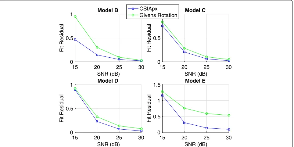
Givens rotation is lossless in the sense that the other end of the communication link can exactly reproduce the mea-sured CSI. It therefore appears that Givens rotation will have higher accuracy than CSIApx, as CSIApx is based on approximation. However, this is only true when the measured CSI is clean, i.e., without any noise. With mea-surement noise and quantization noise, we found that CSIApx actually achieves better accuracy than the Givens rotation, i.e., the CSI with CSIApx follows the shape of the actual CSI more closely than the Givens rotation. From a high level, this is because when fitting a CSI curve, CSIApx serves as a filter and filters out most of the noise, whereas Givens rotation will simply preserve the noise.
15 20 25 30 SNR (dB)
0 0.5 1
Fit Residual
Model B
15 20 25 30
SNR (dB) 0
0.5 1
Fit Residual
Model C
15 20 25 30
SNR (dB) 0
0.5 1
Fit Residual
Model D
15 20 25 30
SNR (dB) 0
0.5 1 1.5
Fit Residual
Model E CSIApx
Givens Rotation
Fig. 14Fit residual comparison with Givens rotation. The comparison between the fit residual achieved by CSIApx and Givens rotation is shown
when running on the synthesized CSI data at four SNR values 15 dB, 20 dB, 25 dB, and 30 dB
comparison, before running the Givens rotation, a low-pass filter is used in an attempt to filter out some noise, as it is expected that such filter will be used in practice. Due to the low-pass filter, only the results of the middle 50 sub-carriers are used in this comparison. The performance of CSIApx is better with the middle 50 subcarriers than with all subcarriers, because the subcarriers near the ends have less constraints in the fitting and have larger errors.
CSIApx will also enjoy a higher compression ration than the Givens rotation. Figure 15 shows the compression ratio for the experimental data. As mentioned earlier the average compression ratio achieved by CSIAPX for the 2 × 2 system in a real-world setting was 7.68. Because
2 3 4 5 6 7 8
Antenna Order 0
2 4 6 8 10
Compression Ratio
CSIAPX vs Givens Rotation
Givens Rotation CSIApx
Fig. 15Compression ratio comparison with Givens rotation. The
comparison between compression ratio for CSIAPx versus Givens Rotation is shown for the experimental data
CSIApx fits each antenna pair individually, hence, it can remain constant even when the number of pairs increases. The compression ratio achieved by Givens rotation on the other hand will keep decreasing as the antenna order increase is approaching 2.
5.4.2 MU-MIMO rate
We further evaluate the fit accuracy by comparing the data rate achieved in a MU-MIMO setting from both CSI-Apx and Givens rotation. Figure16shows the percentage of cases where the normalized rate differences are higher than 3% or lower than−3% when compared against the clean signal. We see that CSIApx outperforms Givens rotation.
6 Conclusion
15 20 25 30
Fig. 16MU-MIMO rate difference comparison with Givens rotation. The percentage of cases where the normalized rate differences are above 3% or
lower than−3% is shown when running CSIApx versus Givens rotation on the synthesized CSI data
Abbreviations
CSI: Channel state information; OFDM: Orthogonal frequency division multiplexing; MU-MIMO: Multi-user multiple-input-multiple-output; SVD: Singular value decomposition
Acknowledgments
The authors greatly appreciate the editor and reviewers for their work.
Funding
This research work was supported by the US National Science Foundation under Grant 1618358.
Availability of data and materials
The data in this work will be made available to the public for free through web access.
Authors’ contributions
Both authors contributed to the work. Both authors read and approved the final manuscript.
Competing interests
The authors declare that they have no competing interests.
Publisher’s Note
Springer Nature remains neutral with regard to jurisdictional claims in published maps and institutional affiliations.
Received: 19 July 2018 Accepted: 19 March 2019
References
1. I. P. .-T. G. AC, Status of Project IEEE 802.11ac (2013).http://www.ieee802.
org/11/Reports/tgac_update.htm. Accessed 15 Sept 2013
2. A. Mukherjee, Z. Zhang, in2016 13th Annual IEEE International Conference on Sensing, Communication, and Networking (SECON). Channel state information compression for MIMO systems based on curve fitting (IEEE, London, 2016)
3. X. Wang, Channel feedback in OFDM systems (2014). Google Patents. US Patent No. 8,908,587. 9 Dec
4. X. Wang, S. B. Wicker, in2013 IEEE Global Communications Conference (GLOBECOM). Channel estimation and feedback with continuous time domain parameters (IEEE, Atlanta, 2013), pp. 4306–4312
5. S. Ferguson, F. Labeau, A. M. Wyglinski, in2010 IEEE 72nd Vehicular Technology Conference-Fall (VTC). Compression of channel state information for wireless OFDM transceivers (IEEE, Ottawa, 2010), pp. 1–5 6. V. P. G. Jiménez, T. Eriksson, A. G. Armada, M. J. F. García, T. Ottosson, A.
Svensson, Methods for compression of feedback in adaptive multi-carrier 4G schemes. Wirel. Pers. Commun.47(1), 101–112 (2008)
7. U. K. Tadikonda, Adaptive bit allocation with reduced feedback for wireless multicarrier transceivers. PhD thesis (2007)
8. V. Pohl, P. H. Nguyen, V. Jungnickel, C. V. Helmolt, in2003 IEEE Global Telecommunications Conference (GLOBECOM). How often channel estimation is needed in MIMO systems, vol. 2 (IEEE, San Francisco, 2003), pp. 814–818
9. K. Huang, R. W. Heath Jr., J. G. Andrews, Limited feedback beamforming over temporally-correlated channels. IEEE Trans. Sig. Process.57(5), 1959–1975 (2009)
10. X. Xie, X. Zhang, K. Sundaresan, in19th Annual International conference on Mobile computing & networking (MOBICOM 2003). Adaptive feedback compression for MIMO networks (ACM, San Diego, 2013), pp. 477–488 11. R. Crepaldi, J. Lee, R. Etkin, S. Lee, R. Kravets, in2012 Proceedings IEEE
International Conference on Computer Communications INFOCOM. CSI-SF: Estimating wireless channel state using CSI sampling & fusion (IEEE, Orlando, 2012), pp. 154–162
12. C. Carbonelli, S. Vedantam, U. Mitra, Sparse channel estimation with zero tap detection. IEEE Trans. Wirel. Commun.6(5), 1743–1763 (2007) 13. F. Wan, W. Zhu, M. Swamy, Semi-blind most significant tap detection for
sparse channel estimation of OFDM systems. IEEE Trans. Circuits Syst. I. Reg. Papers.57(3), 703–713 (2010)
14. M. Duarte, Y. Eldar, Structured compressed sensing: from theory to applications. IEEE Trans. Signal Process.59(9), 4053–4085 (2011) 15. D. Vasisht, S. Kumar, H. Rahul, D. Katabi, inProceedings of the 2016 ACM
16. M. Guillaud, D. T. M. Slock, R. Knopp, in2005 Proceedings of the Eighth International Symposium on Signal Processing and Its Applications, (ISSPA). A practical method for wireless channel reciprocity exploitation through relative calibration (IEEE, Sydney, 2005)
17. A. Mukherjee, Z. Zhang, in2017 IEEE Global Communications Conference (GLOBECOM). Fast compression of OFDM channel state information with constant frequency sinusoidal approximation (IEEE, Singapore, 2017) 18. Z. Zhang, A. Mukherjee, System and method for fast compression of
OFDM channel state information (CSI) based on constant frequency sinusoidal approximation (2017). Google Patents. US Patent No. 9838104. 5 Dec
19. L. Schumacher, Implementation of the IEEE 802.11 TGn Channel Model (2006).http://www.info.fundp.ac.be/~lsc/Research/
IEEE_80211_HTSG_CMSC
20. Y. Xie, Z. Li, M. Li, inProceedings of the 21st Annual International Conference on Mobile Computing and Networking (MOBICOM 2015). Precise power delay profiling with commodity WiFi (ACM, New York, 2015), pp. 53–64 21. N. Ravindran, N. Jindal, Multi-user diversity vs. accurate channel state
information - MATLAB code (2009).http://www.ece.umn.edu/~nihar/