R E S E A R C H
Open Access
Generalized generating function with tucker
decomposition and alternating least squares for
underdetermined blind identification
Fanglin Gu
1*, Hang Zhang
1, Wenwu Wang
2and Desheng Zhu
1Abstract
Generating function (GF) has been used in blind identification for real-valued signals. In this paper, the definition of GF is first generalized for complex-valued random variables in order to exploit the statistical information carried on complex signals in a more effective way. Then an algebraic structure is proposed to identify the mixing matrix from underdetermined mixtures using the generalized generating function (GGF). Two methods, namely GGF-ALS and GGF-TALS, are developed for this purpose. In the GGF-ALS method, the mixing matrix is estimated by the decomposition of the tensor constructed from the Hessian matrices of the GGF of the observations, using an alternating least squares (ALS) algorithm. The GGF-TALS method is an improved version of the GGF-ALS algorithm based on Tucker decomposition. More specifically, the original tensor, as formed in GGF-ALS, is first converted to a lower-rank core tensor using the Tucker decomposition, where the factors are obtained by the left singular-value decomposition of the original tensor’s mode-3 matrix. Then the mixing matrix is estimated by decomposing the core tensor with the ALS algorithm. Simulation results show that (a) the proposed GGF-ALS and GGF-TALS approaches have almost the same performance in terms of the relative errors, whereas the GGF-TALS has much lower computational complexity, and (b) the proposed GGF algorithms have superior performance to the latest GF-based baseline approaches.
Keywords:Blind identification; Generalized generating function; Tensor decomposition; Tucker decomposition; Underdetermined mixtures
1. Introduction
Blind identification (BI) of linear mixtures has recently attracted intensive research interest in many fields of signal processing including blind source separation (BSS). This work is devoted to BI of underdetermined mixtures with complex sources. Underdetermined mix-tures are commonly encountered in many practical applications, such as in the radio communication con-text, where the reception of more sources than sensors becomes increasingly possible with the growth in recep-tion bandwidth. In these applicarecep-tions, one often has to also deal with complex sources. One reason is that the communication signals are usually complex-valued such as the quadrature-amplitude modulation (QAM) signal,
and minimum-shift keying (MSK) signal. Another reason is that frequency domain methods are often used for blind separation or identification from convolutive mix-tures due to its computational efficiency [1,2], while the objective functions used in the frequency domain are usually defined on complex-valued variables.
A large number of methods for BI of underdetermined mixtures start from the assumption that the sources are sparse by nature (i.e., in its own domain such as the time domain) or could be made sparse in another domain (e.g., a transform domain). A predefined transform such as short-time Fourier transform (STFT) or a learned transform using, e.g., simultaneous codeword optimization (SimCO), is usually applied to sparsify the data [3,4] if the signal by nature is not sparse. Due to the sparsity of the sources, the scatter plot typically shows high signal values in the directions of the mixing vectors, which can be local-ized by using some clustering techniques [5,6]. It should
* Correspondence:[email protected]
1
College of Communication Engineering, PLA University of Science & Technology, Nanjing 210007, People’s Republic of China
Full list of author information is available at the end of the article
be noted that although some signals such as speech signals have some degree of sparsity in one domain or another, many other signals such as the majority of communication signals do not possess such a property. Hence, it is ne-cessary to develop BI methods for the underdetermined mixtures that do not impose any sparsity constraint on the sources.
To this aim, many methods for BI of underdetermined mixtures turn to the use of various decomposition methods based on different data structures such as correl-ation [7,8] and higher-order cumulant [9-14] matrices. The main idea of these algorithms is to construct a tensor based on the cumulants of the observations and then to estimate the mixing matrix by the decomposition of such a tensor. This is notably the case for second-order blind identification of underdetermined mixtures (SOBIUM) [7], fourth-order blind identification of underdetermined mixtures (FOBIUM) [9], fourth-order-only blind tification (FOOBI) [10], FOOBI-2 [10], and blind iden-tification of mixtures of sources using Redundancies in the daTa Hexacovariance matrix (BIRTH) [11,12] algo-rithms, which use second-order statistics tensors and fourth- and sixth-order cumulant tensors, respectively. A family of the methods named blind identification of over-complete mixtures of sources (BIOME) is pro-posed in [13], based on the even-order cumulants of the observations. However, all the methods proposed in [7-14] exploit only the statistical information contained in the data measured by second-order or higher-order statistics.
In order to exploit statistical information more effectively, a family of BI approaches was proposed in [15-18] by exploiting the statistical information with the characteristic function (CAF) or generating function (GF). In these works, the authors showed that the mixing matrix can be esti-mated up to trivial scaling and permutation indeterminacies by decomposing the tensor composed of partial derivatives of the GF. It is worth mentioning that the algorithms in [15-17] have been only applied to BI problems involving real-valued sources. In [18], the CAF approach was extended to the case of mixtures of complex-valued sources, which often occurs in digital communications. However, extra effort is required to obtain the correct real and imaginary combination of the mixing matrix since the real and imaginary parts of the mixing matrix are treated separately, leading to an increased computa-tional cost due to the increased dimension of the matrix that needs to be processed. In this paper, we propose the Generalized Generating Function (GGF) to exploit the statistical information carried on the complex ran-dom variable. We show that the proposed GGF can ex-ploit the statistical information carried on complex random variables in a more effective way than the GF presented in [18] due to the algebraic structure adopted
by GGF (as detailed in Algebraic structure based on generalized generating function). Furthermore, a sim-ple method for the mixing matrix estimation is derived based on tensor decomposition where the tensor is composed of the Hessian matrices of the GGF of the observations.
The remainder of this paper is organized as follows. In Problem formulation the BI problem is formulated and relevant assumptions are presented. In Algebraic struc-ture based on generalized generating function we firstly generalize the definition of the GF for complex-valued random variables and then derive the corresponding core equation for BI. In Blind identification based on tensor de-composition, the GGF-ALS and GGF-TALS approaches are developed for the estimation of the mixing matrix. In the GGF-ALS algorithm, the mixing matrix is estimated by directly decomposing the tensor, constructed from the Hessian matrices of the second GGF of the observations, using the alternating least squares (ALS) algorithm. In the GGF-TALS algorithm, the Tucker decomposition is firstly applied to convert the original tensor to a lower-order core tensor, then the mixing matrix is obtained by decomposing the core tensor with the ALS algorithm. Furthermore, the factors of Tucker decomposition are obtained by the left singular vectors of the original tensor’s mode-3 matrix. Computer simulations are used to illustrate the performance of the proposed GGF approaches in Simulations and analysis. Finally, the paper is concluded in Conclusions.
2. Problem formulation
Considering the following linear mixture model
zð Þ ¼t Asð Þ þt wð Þt ð1Þ
where the stochastic vector z(t)∈CQ represents the observation signals, s(t)∈CP contains the unobserved source signals, andw(t)∈CQdenotes additive noise. From now on, the noise w(t) is simply ignored for conveni-ence, except when running computer experiments. The unknown mixing matrix A∈CQ×P characterizes the way that the sources are acquired by the sensors. BI aims to estimate the mixing matrix from the observa-tions based on the assumption that the source signals are statistically independent. The mixing matrix obtained may in turn be used to estimate the original source signals from the observations. In addition, we make the following assumptions:
(i). The mixing matrixAis of full (row) rank.
(ii). The numberPof sources is known.
3. Algebraic structure based on generalized generating function
3.1. Core equation based on generalized generating function For a real stochastic vectorx∈RQ, the GF ϕx(u) obtained by dropping the term of the square root of (−1) in the exponent of a CAF is defined as
ϕxð Þ ¼u E exp uTx
;u∈RQ; ð2Þ
whereu∈RQis an arbitrary vector referred to as a process-ing point [15], and E[ ] denotes an expectation operator. Nevertheless, both the observation vectorzand the mixing matrix A discussed in this paper belong to the complex field. Hence, a definition of GF for complex variables is required. One such definition has been presented in [18] as
ϕzðRð Þu;Ið ÞuÞ ¼E exp R uHz parts from their arguments (i.e., complex-valued vectors) to form a real-valued vector of the same dimension. It is actually defined by assimilating C to R2. Thus the GF of a complex variable in (3) is defined as a function of the real and imaginary parts. In this paper, we generalize the definition of GF for real stochastic vector in (2) to the following complex form
ψzð Þ ¼u E exp uHz
;u∈CQ ð4Þ
Note that the statistical information exploited by GF/ GGF is related to the number of processing points. Theor-etically, a complete statistical description of the probability density function requires the evaluation of the GF/GGF at all (infinitely many) possible processing points. However, this often becomes computationally infeasible. In practice, such statistical information is obtained approximately by the evaluation of GF/GGF at a finite number of processing points. Hence, in comparison with the GF presented in [18], the GGF defined in (4) can exploit the statistical infor-mation carried on the complex variables more effectively when the number of the processing points stays the same, thanks to the incorporation of the imaginary part of the exponent to the function. Furthermore, as compared with the use of the GF in (3), using the GGF in (4) offers a sim-pler way for the estimation of the mixing matrix due to the exploitation of an elegant algebraic structure.
Now, replacingzby its model and neglecting the noise contribution yield
Definingφz(u) = logψz(u), which is often referred to as the ‘second’ GGF, and using the source independence
property, the second GGF of the observations can be rewritten as Consequently, by calculating the derivative of the conju-gate gradient ofφz(u) with respect tou (more details can be found in Appendix 1), we can obtain the following core equation for the Hessian matrixψz(u),
ψzð Þ ¼u Aψs AHu
where (·)*denotes the conjugate operator. It is necessary to point out that ψs(AHu) is a diagonal matrix (more details can be found in Appendix 2).
3.2. Estimatingψz(u)
In this subsection, we discuss how to consistently estimate the Hessian matrixψz(u). Under the ergodicity assumption, the mean value of a random variable can be estimated by a time average. Hence, we can estimate the GGF of the observation vector as
Q× 1 vector can be estimated by
^
Q×Qmatrix can be estimated by
^
Based on the above analysis, the Hessian matrixψz(u) of the second GGFφz(u) can be obtained as
^
4. Blind identification based on tensor decomposition
Tucker decomposition is firstly employed to convert the original tensor as used in the GGF-ALS algorithm to a lower-rank core tensor, and the mixing matrix is then estimated by decomposing the core tensor with the ALS algorithm.
4.1. The GGF-ALS algorithm
Evaluating the Hessian matricesψz(u) of GGF at a series of processing points u1,u2,...,uK and using Equation (7), one can obtain the following joint diagonalization (JD) problem
(
ψzð Þ ¼u1 Aψs AHu1
AH
⋮
ψz uKÞ ¼Aψs AHuK
AH
ð9Þ
in whichψs(AHuk) is diagonal,k=1,…,K. The problem we need to address is to estimate the mixing matrixAbased on the set {ψz(u1),⋯,ψz(uK)}. For the determined/overde-termined case, it is obvious that JD methods, such as the AC-DC method [19], can be used to estimate the mixing matrix. However, this method does not work whenQ < P
i.e., in the underdetermined case.
As shown in [7], the JD problem (9) can be seen as a particular case of the parallel factor (PARAFAC) decom-position, also known as canonical decomposition (CAND), of the third-order tensor M∈CQQK built by stacking the Kmatrices ψx(uk) along the third mode. Specifically, the tensor M∈CQQK is built by stacking ψz(u1),ψz (u2),...,ψz(uK) as follows:ðMÞijk¼ðψzð Þuk Þij,i =,…,Q,j =
1,…,Q,k= 1,…,K. Define a matrixD∈CK×Pby (D)kl= (ψs(AH
uk)ll,l= 1,…,P,k= 1,…,K. Then we have
mijk ¼
XP l¼1aila
jldkl; ð10Þ
which we write as
M ¼XPl¼
1al∘a
l∘dl; ð11Þ
where º denotes the tensor outer product, andalanddl represent thelth column ofAand D, respectively. In this way, the mixing matrixA can be estimated by solving the following problem. Given the third-order tensor
M∈CQQK, we can compute its CAND withP compo-nents of the rank-one tensors that best approximates M, i.e.,
min
A;D M−
XP p¼1ap∘a
p∘dp
2
F; ð12Þ
where‖‖Fis the Frobenius norm.
Several algorithms exist for the computation of tensor decomposition. The standard way for computing the tensor decomposition is by using an ‘ALS’ algorithm [20]. Several improved versions, such as the enhanced
line search (ELS) [21] and extrapolating search direction (ESD) [22], are proposed to accelerate the rate of con-vergence of the ALS. Hence, the ALS is chosen here to compute the CAND.
To a large extent, the practical importance of tensor decomposition stems from its uniqueness properties. It is clear that the tensor decomposition can only be unique up to a permutation of the rank-1 terms and scaling of the factors of the rank-1 terms. Therefore, we consider the tensor decomposition (11) as essentially unique if any other matrix pairA’and D,’that satisfies (11) is related to AandDvia
A¼A0PΔ1; D¼D0PΔ2 ð13Þ
with Δ1,Δ2∈CP×P being diagonal matrices, satisfying
Δ1Δ1Δ2=I, andP∈RP×Pbeing a permutation matrix.
The k-rank. The Kruskal rank or k-rank of a matrixA, denoted by κA, is the maximal number λ such that any set ofλcolumns ofAis linearly independent.
Theorem 1.The tensor decomposition of(11)is essen-tially unique if[23]
2κAþκD≥2ðPþ1Þ ð14Þ
We call a property generic when it holds with probabil-ity one. Generically, the mixing matrix is of full rank and of full k-rank when the parameters it involves are drawn from continuous probability densities. Hence, in practice, κA= min(Q,P)andκD= min(K,P).
In summary, we come to the following conclusion: whenQ≥P,P≥2, then the generic essential uniqueness is guaranteed forK≥2; whenQ<Pand ifK≥P, then the generic essential uniqueness is guaranteed forP≤2Q−2, if
K<P, then the generic essential uniqueness is guaranteed forP<Q−1 +K/2.
4.2. The GGF-TALS algorithm
In order to ensure the GGF-ALS algorithm has robust performance, a large value is often chosen for K in the tensor M∈CQQK. Nevertheless, this will lead to a heavy computational load. To reduce the computational complexity, the Tucker decomposition [23-25] is firstly applied to represent the tensor M as a lower-rank core tensor, whose size is much smaller than the tensor M. Then the ALS algorithm is used to perform the CAND of the core tensor. In this way, the computational complexity can be reduced dramatically.
Matricization. Matricization, also known as unfolding or flatting, is the process of turning an N-way tensor into a matrix. The mode-n matricization of a tensor
F ∈CI1I2⋯IN is denoted by F(n) which arranges the
matrix, that is, the tensor element (i1,⋯,iN) is mapped to the matrix element (in,j) where
j¼1þX
k¼1
k≠n N
ik−1 ð ÞJk
with
Jk ¼
Y
m¼1
m≠n k−1
Im
The n-rank. Let F be an Nth-order tensor of size
I1×I2⋯×IN. Then the n-rank of F , denoted by ranknð ÞF , is the column rank of F(n). In other words, if
we letrn¼ranknð ÞF forn = 1,…,N, then we can say that F is a rankr1,⋯,rNtensor.
The n-mode product. The n-mode (matrix) product of a tensor F ∈CI1I2⋯IN with a matrix UJIn is
de-noted by F nU and is of size I1×⋯×In−1×J×In+ 1×⋯IN. Elementwise, we have
F nU
ð Þi1⋯in−1jinþ1⋯iN ¼XIn
in¼1fi1i2⋯iNujin
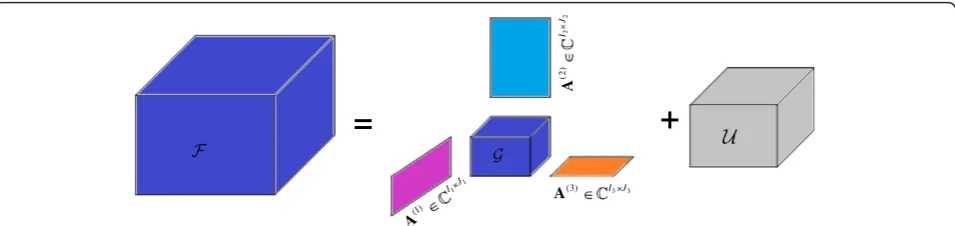
Tucker decomposition is a form of higher-order principal component analysis (PCA). It decomposes a tensor into a core tensor multiplied by a matrix along each mode as shown in Figure 1. Thus, in the three-way case whereF ∈CI1I2I3, we have
F ¼ G1Að Þ12Að Þ23Að Þ3 þ U
¼XJ1
j1¼1
XJ2
j2¼1
XJ3
j3¼1
gj
1j2j3 a
1
ð Þ j1 ∘a
2
ð Þ j2 ∘a
3
ð Þ j3
þ U;
ð15Þ where G∈CJ1J2J3 is the core tensor; Að Þ1 ∈CI1J1;Að Þ2 ∈CI2J2;Að Þ3 ∈CI3J3 are the factor matrices (which are
usually column unitary for real-valued data) and can
be thought of as the principal components in each mode; andU∈CI1I2I3represents errors or noise.
With the help of Tucker decomposition, the tensor
M, which is composed of the Hessian matrices ψz(uk) of the second GGF of the observations, can be com-pressed. Since the mixing matrix A is of full rank and the Hessian matrices ψs(AHuk) of the second GGF of the sources are diagonal, the mode-n(n= 1, 2, 3) matri-ces of tensor MareM(1)∈CQ×QK, M(2)∈CQ×QK, and M(3)∈CK×QQ respectively. Meanwhile, the n-rank of theM(1)andM(2)is
rank1ðMÞ ¼rank2ðMÞ ¼rankMð Þ1
¼rankMð Þ2¼Q ð16Þ
On the other hand, if we assume rank3ðMÞ ¼L and
L≤K, then Mis a rank-(Q,Q,L) tensor. Thus, the Tucker decomposition of tensor M is the so-called Tucker1 de-composition [23]
M ¼ T 1I2I3G ð17Þ
whereT ∈CQQLis the core tensor,I∈RQ×Qis an iden-tity matrix, andG∈CK×Lis a column-unitary matrix. This is equivalent to a standard two-dimensional PCA since
Mð Þ3 ¼GTð Þ3; ð18Þ
whereT(3)∈CL×QQis the mode-3 matrix of core tensorT. It is obvious that (18) corresponds to the PCA of M(3). Therefore,G∈CK×Lconsists of theL-leading left singular vectors of M(3). Since K>L and G is a column-unitary matrix, it is straightforward to derive
Tð Þ3 ¼GHMð Þ3 ð19Þ
Therefore, the core tensor can be obtained by
T ¼ M 1I2I3GH ð20Þ
Because the first and second factors of the Tucker decomposition in (17) are identity matrices, the core tensor T ∈CQQL is also a symmetric tensor [23], as
=
+
1 1
(1) I J
A
22
(2
)
IJ
A
3 3
(3) I J
A
for the tensorM∈CQQK and the CAND of the core tensor is as follows
T ¼XPl¼1
al∘a―l∘d―l; ð21Þ
wherealanddlare thelth column ofAandD, respectively. The CAND process can also be implemented by the ALS algorithm. Nevertheless, our goal is to estimate the mixing matrixA, whereas the CAND of core tensor T ∈CQQL only conduces A. Hence, it is necessary to derive the mixing matrixA based on A. Since the first and second factors of Tucker decomposition (17) are identity matrices, it is straightforward to derive
A¼IA― ¼ A― ð22Þ
4.3. Computational analysis
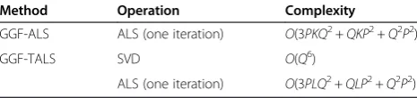
In this subsection, we aim at giving an insight into the numerical complexity of the proposed algorithm. For the GGF-ALS algorithm, the ALS algorithm is directly used to decompose the tensor M∈CQQK; therefore, the com-putational complexity is O(3PKQ2+QKP2+Q2P2) per it-eration. For the GGF-TALS algorithm, the computational complexity is dominated by the Tucker decomposition of the original tensorM∈CQQK (realized by the singular-value decomposition (SVD) of the mode-3 matrix M(3)) and the decomposition of the core tensor T ∈CQQL using the ALS algorithm. Therefore, the computational complexities for these two operations per iteration are
O(Q6) and O(3PLQ2+QLP2+Q2P2), respectively. Table 1 shows the computational complexity for the GGF-ALS, and GGF-TALS methods.
It is worth mentioning that a large value is usually chosen for the number of processing pointsKin order to accumu-late sufficient statistical information from data, while the rank of the core tensor orderLis often chosen to be much smaller than K. For example, K= 100, L = 8 are chosen typically in our simulations as shown in the next section. The SVD is required to be calculated only once, whereas the ALS algorithm needs multiple iterations to achieve convergence, for example, 1,000 iterations as in our experi-ments. Moreover, the number of sourcesPand the number of sensorsQare usually small, for example,P =4, Q =3 in our simulations. For these reasons, it can be readily derived
from Table 1 that the computational cost of the GGF-TALS algorithm is, in practice, much lower than that of the GGF-ALS algorithm (note that the complexity of SVD becomes negligible in this case).
5. Simulations and analysis
In this section, simulations are provided to illustrate the performance of the proposed GGF approaches for underdetermined mixtures of complex sources. The performance of the tested algorithms is evaluated and compared in terms of the relative error performance index (PI) versus the sample size and the signal-to-noise ratio (SNR) of the observations. Here the relative error PI is defined as [7] PI ¼ EfjjA−A^jj=jjAjjg, in which the norm is the Frobenius norm andÂrepresents the optimally or-dered and scaled estimate of the mixing matrixA.
The experiments refer to the scenario that P = 4 nar-rowband source signals are received by a uniform circular array (UCA) with Q = 3 identical sensors of radius Ra Considering a free space propagation model, the entries of the mixing matrixAare given by
aqp¼ exp 2πj αqcosθp cos ϕp þβqcos θp sin ϕp
whereαq= (Ra/λ)cos(2π(q−1)/Q),βq= (Ra/λ)sin(2π(q−1)/Q), and j¼pffiffiffiffiffiffi−1. We haveRa/λ= 0.55. The direction of arrival (DOA) of the different sources are given by θ1= 3π/10, θ2= 3π/10,θ3= 2π/5, θ4= 0 andϕ1= 7π/10,ϕ2= 9π/10, ϕ3= 3π/5, ϕ4= 4π/5. The sources are unit-variance 4-QAM with a uniform distribution, shaped by a raised cosine pulse shaping filter with a roll-off ρ = 0.3. All sources have the same symbol durationT= 4Te, where
Teis the sample period. The observations are contami-nated by additive zero-mean complex Gaussian noise.
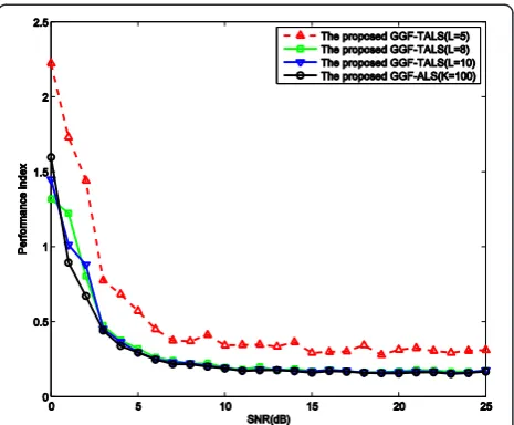
First, we compare the performance of the GGF-ALS algorithm with that of the GGF-TALS algorithm and inves-tigate the influence of the rank of the core tensorLon the performance of the GGF-TALS algorithm. To this end, the following two simulation experiments are conducted. In the first simulation, we evaluate the performance of the GGF-TALS algorithm with different core tensor rankLfor a fixed number of processing pointsK, and compare it with GGF-ALS with the same number of processing points. In this simulation, K is chosen to be 100 for the GGF-ALS algorithm, both the real and imaginary parts of processing points are randomly drawn from [−1; 1], the SNR of the observations ranges from 0 to 25 dB, and the number of samples is 4,000. The core tensor rank for the GGF-TALS algorithm is chosen asL= 10,8,5, respectively. The thresh-old value described in (12) to stop the ALS algorithm is 10−5, and 100 Monte Carlo experiments are run.
The average performance of the GGF-TALS algorithm versus the core tensor rank for a fixed number of pro-cessing points is shown in Figure 2. We can see that the
Table 1 Computational complexity of GGF-ALS, GGF-TALS methods
Method Operation Complexity
GGF-ALS ALS (one iteration) O(3PKQ2+QKP2+Q2P2)
GGF-TALS SVD O(Q6)
performance curves of the GGF-TALS and that of the GGF-ALS almost coincide when the rank of the core tensor is larger than 8, whereas the performance of the GGF-TALS algorithm slightly deteriorates when the rank of the core tensor is less than 8. This indicates that the GGF-TALS algorithm maintains the identifica-tion accuracy offered by GGF-ALS despite the fact that the core tensors used by GGF-TALS have a much lower rank than that of the original tensor used by GGF-ALS.
In the second experiment, we investigate the per-formance of the GGF-TALS algorithm with different
number of processing points K when the rank of the core tensor L is fixed. The simulation conditions are the same as those in the previous simulation except the number of processing points for the GGF-ALS algo-rithm which are 20, 40, and 100 respectively, and the rank of the core tensor for the GGF-TALS which is 8. The average performance of the GGF-TALS versus the number of processing points for the fixed number of the core tensor rank is shown in Figure 3.
We can see that the average performance of GGF-TALS is consistent with that of GGF-ALS when both algorithms use the same number of processing points. For instance, when the number of processing points is 100, the perform-ance of TALS is close to the performperform-ance of GGF-ALS, so is forK= 40. Therefore, the GGF-TALS algorithm consistently offers similar performance to GGF-ALS when the number of processing points is varied.
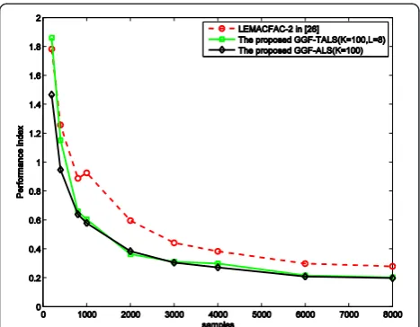
Second, we compare the performance of the GGF-ALS and GGF-TALS algorithms with that of the latest GF-based BI algorithm. Here, the LEMACFAC-2 in [18] is chosen as the baseline algorithm. The number of processing points and the value of processing points for the ALS, GGF-TALS, and LEMACFAC-2 are the same. Specifically, the number of processing points is 100, both the real and imaginary parts of processing points are randomly drawn from [−1; 1], and the rank of the core tensor is 8. The threshold value described in (12) to stop the LM algorithm [26] exploited in LEMACFAC-2 method is also 10−5.
Figure 4 shows the PI of the tested algorithms as a function of the SNR when 4,000 samples are used. It can be seen from this figure that the performance of the GGF-ALS is consistent with that of the GGF-TALS, and both perform better than LEMACFAC-2. Figure 5 shows
Figure 2Performance of GGF-TALS versus core tensor order for a fixed number of processing points.The results for GGF-ALS are also shown for comparison.
Figure 3The performance of GGF-TALS versus the number of processing points.The results for GGF-ALS are also shown for comparison.
the PI of the tested algorithms as a function of the number of data samplesNwhen the SNR is equal to 20 dB. Again, the LEMACFAC-2 underperforms the GGF-ALS and the TALS algorithms, and the ALS and the GGF-TALS have almost the same performance. This confirms that the GGF algorithms perform better than the method based on the GF defined in (3) in exploiting the statistical information carried on the complex variables when using the same number of processing points.
6. Conclusions
We have presented two algorithms, namely, GGF-ALS and GGF-TALS, for blind identification from underdetermined mixtures of complex sources using the second GGF of the observations. In the GGF-ALS algorithm, the mixing matrix is estimated by directly using the ALS algorithm to decompose the tensor constructed from the Hessian matrices of the second GGF of the observations. The GGF-TALS algorithm is an improved version of the GGF-ALS algorithm, where the Tucker decomposition is first used to convert the original tensor into a lower-rank core tensor, and the mixing matrix is then estimated by applying the ALS algorithm to the core tensor. Simulation results have shown that (a) the proposed GGF-ALS and GGF-TALS approaches have almost the same performances in terms of the relative errors, whereas the GGF-TALS has a much lower computational complexity, and (b) the proposed GGF algorithms have superior performance to the latest GF-based BI ap-proaches, since the GGF algorithms can exploit the statistical information carried on complex variables in a more effective way.
Appendix 1
In this appendix, we show the computational details of the core equation in Equation 7. First, the differentiation of (6) with respect tou*gives Second, the differentiation of (23) with respect touTgives
∂φzð Þu In a more compact form, we can obtain the core equation
ψzð Þ ¼u Aψs AHu
AH ð25Þ
Appendix 2
Let ϕsð~uÞ denote the characteristic function of the source signalss(t). Due to the statistical independence of the elements ofs(t) = [s1(t),⋯,sP(t)]T, we have for the second characteristic functionφs(ũ), we have
φsð~uÞ ¼φs1ð Þ þu~1 φs2ð Þ þu~2 ⋯þφsPð Þ~uP ð27Þ
Consequently, the Hessian matrix ψs(ũ) can be easily obtained as
where diag(·) represents an operator forming a diagonal matrix by assigning its arguments to the entries of the main diagonal.
Competing interests
The authors declare that they have no competing interests.
Acknowledgments
This work is supported in part by Natural Science Foundation of China under grant 61001106 and National Program on Key Basic Research Project of China under grant 2009CB320400, and Engineering and Physical Science Research Council of the UK under grant EP/H050000/1. The authors would like to thank the anonymous referees for their constructive comments for improving this paper and Dr. Mark Barnard for proofreading the manuscript.
Author details
1College of Communication Engineering, PLA University of Science & Technology, Nanjing 210007, People’s Republic of China.2Department of Electronic Engineering, University of Surrey, Guildford GU2 7XH, UK.
Received: 2 November 2012 Accepted: 21 June 2013 Published: 1 July 2013
References
1. B Chen, AP Petropulu, Frequency domain blind MIMO system identification based on second- and higher order statistics. IEEE Trans. Signal Process.
49(8), 1677–1688 (2001)
2. K Rahbar, JP Reilly, A frequency domain method for blind source separation of convolutive audio mixtures. IEEE. Trans. Speech Audio Process
13(5), 832–844 (2005)
3. A Aissa-EI-Bey, N Linh-Trung, K Abed-Meraim, A Belouchrani, Y Grenier, Underdetermined blind separation of nondisjoint sources in the time-frequency domain. IEEE Trans. Signal Process.55(3), 897–907 (2007)
4. W Dai, T Xu, W Wang, Simultaneous codeword optimization (SimCO) for dictionary update and learning. IEEE Trans. Signal Process.
60(12), 6340–6353 (2012)
5. P Bofill, M Zibulevsky, Underdetermined blind source separation using sparse representations. Signal Process.81, 2353–2362 (2001)
6. C Févotte, SJ Godsill, A Bayesian approach for blind separation of sparse sources. IEEE Trans Audio Speech Lang Process14(6), 2174–2188 (2006) 7. LD Lathauwer, J Castaing, Blind identification of underdetermined mixtures
by simultaneous matrix diagonalization. IEEE Trans. Signal Process.
56(3), 1096–1105 (2008)
8. P Tichavský, Z Koldovský, Weight adjusted tensor method for blind separation of underdetermined mixtures of nonstationary sources. IEEE Trans. Signal Process.59(3), 1037–1047 (2011)
9. A Ferréol, L Albera, P Chevalier, Fourth-order blind identification of underdetermined mixtures of sources (FOBIUM). IEEE Trans. Signal Process.
53(5), 1640–1653 (2005)
10. LD Lathauwer, J Castaing, JF Cardoso, Fourth-order cumulant-based blind identification of underdetermined mixtures. IEEE Trans. Signal Process.
55(6), 2965–2973 (2007)
11. L Albera, A Ferreol, P Comon, P Chevalier,Sixth order blind identification of under-determined mixtures (BIRTH) of sources. Proceedings of the 4th International Symposium on Independent Component Analysis and Blind Signal Separation (Nara, 2003), pp. 909–914
12. ALF de Almeida, X Luciani, P Comon,Blind identification of underdetermined mixtures based on the hexacovariance and higher-order cyclostationarity. IEEE Workshop on Statistical Signal Processing (Cardiff, UK, 2009), pp. 669–672 13. L Albera, A Ferréol, P Comon, P Chevalier, Blind identification of over-complete
mixtures of sources (BIOME). Lin. Algebra Appl.391, 1–30 (2004)
14. A Karfoul, L Albera, G Birot, Blind underdetermined mixture identification by joint canonical decomposition of HO cumulants. IEEE Trans. Signal Process.
58(2), 638–649 (2010)
15. A Yeredor, Blind source separation via the second characteristic function. Signal. Process.80(5), 897–902 (2000)
16. E Eidinger, A Yeredor, Blind MIMO identification using the second characteristic function. IEEE Trans. Signal Process.53(11), 4067–4079 (2005) 17. P Comon, M Rajih, Blind identification of underdetermined mixtures based
on the characteristic function. Signal. Process.86(9), 2271–2281 (2006)
18. X Luciani, ALF de Almeida, P Comon, Blind identification of underdetermined mixtures based on the characteristic function: the complex case. IEEE Trans. Signal Process.59(2), 540–553 (2011)
19. A Yeredor, Non-orthogonal joint diagonalization in the least-squares sense with application in blind source separation. IEEE Trans. Signal Process.
50(7), 1545–1553 (2002)
20. LD Lathauwer, BD Moor, J Vandewalle, On the best rank-1 and rank-(R1, R2,…, RN) approximation of higher-order tensors. SIAM J. Matrix Anal. Appl.21,
1324–1342 (2000)
21. D Nion, LD Lathauwer, An enhanced line search scheme for complex-valued tensor decompositions: application in DS-CDMA. Signal Process.
88(3), 749–755 (2008)
22. Y Chen, D Han, L Qi, New ALS methods with extrapolating search directions and optimal step size for complex-valued tensor decompositions. IEEE Trans. Signal Process.59(12), 5888–5898 (2011)
23. TG Kolder, BW Bader, Tensor decompositions and applications. SIAM Rev.
51(3), 455–500 (2009)
24. G Bergqvist, EG Larsson, The higher-order singular value decomposition: theory and an application. IEEE Signal Process. Mag.27(3), 151–154 (2010) 25. G Zhou, A Cichocki, Fast and unique tucker decompositions via multiway
blind source separation. Bull. Pol. Acad. Sci.60(3), 389–405 (2012) 26. P Comon, X Luciani, ALF de Almeida, Tensor decomposition, alternating
least squares and other tales. J. Chemometr.23, 393–405 (2009)
doi:10.1186/1687-6180-2013-124
Cite this article as:Guet al.:Generalized generating function with tucker decomposition and alternating least squares for
underdetermined blind identification.EURASIP Journal on Advances in Signal Processing20132013:124.
Submit your manuscript to a
journal and benefi t from:
7Convenient online submission
7Rigorous peer review
7Immediate publication on acceptance
7Open access: articles freely available online 7High visibility within the fi eld
7Retaining the copyright to your article