Modeling the Behavior of
Large Software Projects
Dana S. Borger
MladenA. Vouk
Center for Communications and Signal Processing
Department of Computer Science
North Carolina State University
ABSTRACT
This report is based on the M.S. thesis written by Dana S. Borger under the direction of Mladen A. Vouk (NCSU, Dept. of Computer Science, May 1991).
The report describes an approach to modeling large software project behavior. The model assumes a phased software development process which is driven by milestone dates. The process is applied to overlapping projects that correspond to the releases of a single software product. Enhancements are implemented in the product as a large number of software components developed in parallel. A certain number of the components must complete each process phase for the product release to attain that phase milestone. The model incorporates Parkinson's Law and the Deadline Effect. The product component life-cycle phase durations are treated as stochastic variables. The durations are related to the time available to a planned milestone date using a regression function. A linear regression model is used to demonstrate the model's adequacy in an observed development environment. The model is evaluated using both empirical project data and simulations. Simulations also serve as a means of investigating non-analytical effects, such as schedule slippages. Empirical results indicate that the model ,-,mbe usedby software managers and software developers to predict the finish behavior of a project for anylife-cycle phase. Such predictions could aid in analyzing risks associated with not meeting planned project deadlines. The model is expandable and programmable, helping to ensure that the model paradigms will be investigated further, and can be adapted and instituted in different
CCSP-lR-91/19/Modeling Behaviorof Large Software Projects/NCSU.CSC/DSB .MAV11une-1991
TABLE OF CONTENTS
Page
LIST OF TABLES · .. · · · ·· · ·· · · ··· · ·· · .· · · ·· · ·· · iii
LIST OF FIGURES iv LIST OF SYMBOLSAND ABBREVIAnONS · · · ·· · · · .. ·· ·· · VI 1 INTRODUcnON · .. · · .. · .. · · ·· · . ·· · ·· · 1
1.1 Goals of this Study · ··· 3
1.2 Model Motivation · ·. · · ·· · ·· · · ·· .· .· · ·· . 5
1.3 Review of Past Work · · . · .· · · .· · · ·· · .· · 9
1.3.1 Software Schedule Estimation Mooels · · .. · 9
1.3.2 Parkinson's Law and the Deadline Effect... 11
1.4 Scope of this Study 14 1.5 Overview of the Study... 15
2 MODaDEvaGPMENT 17 2.1 Model Definitions and Assumptions... 17
DEF'IN'fTIONS ...•... 17
ASSUM¥fIONS .. . . .. . . •. . . 19
2.2 Detailed Descriptionof the Development Environment. . .. .. . . .. . . . .. . . .. . . ... 22
DESCRIPTION OF THE LIFE-CYCLE PHASES 24 2.3 The Single-Variable Model... 27
2.3.1 Model Notation and Definitions... 27
2.3.2 Calculating the Distribution of Finish Times... ~. 2.3.3 The Expected Values of Durations and Finish Times... ' 2.3.4 Applying Least Squares Linear Regression... -: THE SLOPE OF THE REGRESSION LINE . 2.3.5 Estimating the Variances of Duration and Finish Times . 2.4 The Effect of Schedule Changes . 3 MODEL EVALUATION . 3.1 Model Performance on Simulated Data . 3.1.1 A Simulation with No Schedule Changes... ' 3.1.2 Simulating Effects of a Schedule Change.. . . . .. ... .. . . .. . . ... .. . .. . . .. . . . ... 44
3.2 Using the Model to Describe Historical Data 48 3.2.1 Discussion of the Historical Data. . .. .. . .... . . .. . . .. . .... . .. . . . ... . .. . . .. . . ... 48
3.2.2 Linear Regression Analysis. 50 ANALYSISOF THE PARAMETERESTIMATES... 53
NEW PROGRAMS . . . .. . . .. . .. . . .. . . 54
CARRY-OVERPROGRAMS. 55 TESTING THE REGRESSION ASSUMPTIONS... . . . .. . . .. . . .. . 55
3.2.3 Another Data Partitioning Scheme. . . .. . . .. . . .. .. . .. . . .. . . .. . 58
DISCUSSION OF THE TwO MODELS
64
4 CONCLUSION · · .. . . . .. . .. . . .. ... . . .. .. .. . .. . . .. . .. . 664.1 Summa.ry · · ·· . .. . . .. . . .. .. .. . .. .. .. . ... . .. . .. . . .. . . .. . .. . . .. . .. . 66
4.2 Recommendations for Future Research 68 5 REFERENCES 71 APPENDIX I: CONFIDENCE INTERVALS FOR LSQ
m...
73CCSP-TR-91/19/Modeling Behavior of Large SoftwareProjects/NCSU.CSC/DSB .MAV/June-1991
LIST OF TABLES
Page Table 3-1 Summary of input parameters for the simulation 42 Table 3-2 Summary of input parameters for the schedule slip simulation... 44 Table 3-3 Summary statistics for program finish time for programs inProject 1. . . .. 50 Table 3-4 Regression summary for program duration vs. start time for Project 1. . . .. 54 Table 3-5 Regression summary for program duration vs. start time for programs
in Project 1, with the new partitioning of carry-over programs. 60
CCSP-TR-91/19/Modeling Behavior of Large Software Projects/NCSU.CSC/DSB.MAV/1une-1991
LIST OF FIGURES
Page Figure 1-1 Figure 1-2 Figure 1-3 Figure 1-4 Figure 2-1 Figure 2-2 Figure 2-3 Figure 2-4 Figure 3-1 Figure 3-2 Figure 3-3 Figure 3-4 Figure 3-5 Figure 3-6 Figure 3-7 Figure 3-8Scatterplot of component duration vs. start time for componentsin
Project 1. 6
Histogram of start time (a) and finish time (b) for componentsin
Project 1. 7
Cumulative frequency plot for component finish times for
com-ponents in Project 1. .. . . .. . .. . . 8
Example of a partition of a software developer's time. 12 The software development process... 23
illustration of overlapping projects in the environment. . . .. 26
Defined linear relationship between program starting time and duration. . . .. . . .. 31
illustration of re-applying the model after a schedule change. 38 Histogram of actual program start times in Project
1...
41Histogram of simulated program finish times... 42
Cumulative frequency plot of simulated program finish times. . . .. 43
Histogram of actual program fmish times in Project 1... 43
Cumulative frequency plot of actual program fmish timesin Project 1 . .. 44
Histogram of simulated program fmish times, with no slip inthe schedule. 46 Histogram of simulated program finish times, with a 5 unit slip in the schedule announced at timeO... ·... 46
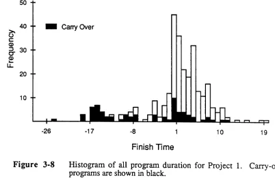
Histogram of all program duration for Project
1... 49
Figure 3-9.1 Scatterplot of program duration vs. start time for Project 1. . . .. 51
Figure 3-9.2 Results of fitting equation 3.1. 54 Figure 3-10 Histogram of the residuals from the full model regression for Project 1. 56 Figure 3-11 Normal probability plot of the residuals from the full model
regression for Project
1...
57
CCSP-TR-91/19/Modeling Behavior of Large Software Projects/NCSU.CSC/DSB .MAV/June-1991
LIST OF FIGURES
(continued)
Page Figure 3-12
Figure 3-13
Figure 3-14 Figure 3-15
Figure 3-16
Figure 3-17
Figure 3-18
Figure 3-19
Figure 4-1
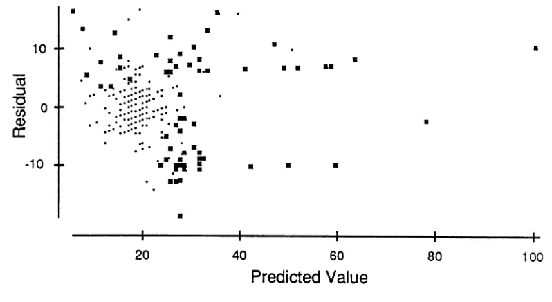
Scatterplot of the residuals vs. the predicted.values from the full
model regression for Project 1 ~. .. . . .. . . .. . 57 Scatterplot of the Cook's Di vs. observation number from the full
model regression for Project 1... 58 Results of fitting equation 3.11... .... . .. .. .... . ... . .. . ... . . .. . . .. . ... . 60 Histogram of residuals from the modelin3.11 for Project 1 with the
new division of carry-over programs. .. .. . . .. . . .. . . .. . . . .. . . .. . . . .. . . .. . 61 Normal probability plot of the residuals from the modelin3.11 for
Project 1 with the new division of carry-over programs. 62 Scatterplot of the residuals vs. predicted values from the model in
3.11 for Project 1 with the new division of carry-over programs 62 Plot of the residuals by group from the model in 3.11 for Project 1
withthe new division of carry-over programs. .. . . .. . . . .. . . . .. . . . .. . . .. . 63 Plot of the Cook's Di statistic by group from the modelin3.11 for
Project 1 with the new division of carry-over programs.... 63 Example plots of times programs achieved various milestones
versus the time they achieved the first milestone. 69
ccsr-
TR-91/19/ModelingBehavior of Large Software Projects/NCSU.CSC/DSB.MAVIJune-1991LIST OF SYMBOLS AND
ABBREVIATIONS
SYMBOL / ABBREVIATION DESCRIPTION
CCX:OMO .
SLIM .
X .
xorxi .
y .
y or yi .
Z .
Zorzi .
pmf .
CI() • • • • • • • • • • • • • • • • • • • • • • • • • • • • • • • • • • • • • • • • • • N 0• • • • • • • • • • • • • • • • • • • • • • • •
Uv or U I V=v .
P(U=u) .
Pu(u) .
Fu(t) ·
E[U] o • • • • • • • • •
Constructive Cost Model.
Putnam's macro software sizing and estimating model.
Random component start time. An observed component start time. Random component phase duration. An observed component duration. Random component fmish time. An observed component fmish time. "probability mass function"
Infinity,
Number of componentsin a software product. Any random variable U given that another random variableV has taken the value v.
The probability that a random variable U takes the value u.
The pmf of a random variable U evaluated at u. Note that P(U=u) = Pu(u).
Cumulative pmf of a random variable U evaluated att
The expected value of a random variableU.
Regression function of Y (duration) on X (start time).
Intercept for the linear regression function. Slope for the linear regression function; a~
o.
General linear model with 1 quantitative variable,
80
is the intercept,81is the slope,
£i is
a
random variable (error term) with meanO. The variance of£i andYi.An estimate of
80,
anestimate ofB1, anestimate of(]'2, etc.
d .
a .
Yi =
Bo
+81Xi +£i 0• • • • •0'2 .••.•...••.•..•••....•..•••...•...•...
" " "2
80, 31, c-, etc .
-
u... The sample mean of a given number ofobservations of the random variableU.
E[U I V=v] orE[U Iv]
0.. .
The conditional expected value of a random variableUgiven that a random variableV has taken the value v.L
f(x) "sum f(x) overallvalues ofx"x
L
f(x)... "sum f(x) over all possible values of x, x~ y"xSy
D(x)
=
E[Y I X=x] .CCSP-TR-91/19/Modeling Behavior of Large Software Projects/NCSU.CSC/DSB.MAVIJune-1991
LIST OF SYMBOLS AND
ABBREVIATIONS
(continued)
SYMBOL / ABBREVIATION DESCRIPTION
HO, Ha . . •• . • •• . . • •. . • • • . . • •. . • • • . • • • •. . • • • Null hypothesis, alternate hypothesis.
ex •••••••••••••••••••••••••••••••••••••••••.• Level of significance used in a confidence interval or hypothesis test
r2 •. .... •..•... . .••.... .. .... . .. .... .•... . .. Coefficient of determination in least squares regression.
df . . .. . . .. . . .. . . .. . . . .. . . .. . . .. . . .. "degrees of freedom" SS(Res) ~ "residual sum of squares"
Q. ... .. .. . ... . . .. .. . .. .. . .... . .... . .. .. . .. . . Difference in residual sums of squares from two least squares regression model fits.
ta,v ...••..••.•••..•..•...•..••...••..•• a percentile of the student's t distribution with v
degrees of freedom.
teaIc .••••..•••....••..• ····•·•••···••••·• A calculated t statistic.
Fa,Vl ,V2. . . ••.•....••...•....• .•....• apercentile of the F distribution withVI numerator andV2denominator degrees of freedom.
Feale · · · A calculated F statistic.
Cook's Di A statistic used to measure potential influence of the ithobservationinleast squares regression.
CCSP-TR-91/19/Modeling Behaviorof Large Software Projects/NCSU.CSC/DSB.MAVIJune-1991
1
INTRODUCTION
Schedule estimation lies at the heart of every software development project. Scheduling and planning playa significant role in successfully delivering software products on time and within budget. Empirical and theoretical schedule estimation models for software development (e.g., COCOMO [Boehm, 1981]) can be applied during the initial stages of a project. These models operate on initial estimates of the product attributes (e.g., lines of code), so the accuracy of the schedules they produce varies with the precision of the estimates. The interpretation of the term "accuracy" may become unclear when one considers the fact that different schedule estimates can produce different project behavior [Abdel-Hamid-Madnick, 1986]. For example, ifthe time needed to develop a software product is overestimated, then the project may progress more slowly than if it had been underestimated. Other factors, like the availability of resources, also affect project progress.
CCSP-TR-91/19/Modeling Behavior of Large Software Projects/NCSU.CSC/DSB .MA VIJune-1991 2
effect to partially describe project behavior after a schedule has been set. This study examines the impact of the schedule on the project itself. Some other studies have also investigated this concept quantitatively using simulations (e.g., [Abdel-Hamid-Madnick,
1983, 1986]).
Software engineering, as it is practiced today, is largely a problem-solving and social activity; many people .communicate and cooperate to design, implement and test software systems to be used by people. The dynamics of social interactions are hard to predict. The relationships between people, and with the work they perform, create the difficulties associated with estimating a software project schedule. The dynamics include "feedback loops", resource utilization, productivity, and so on. Feedback loops occur when eventsin
the present have a direct impact on future work. An example is design rework due to a design flaw discovered during coding. A broader example is future schedule estimation based on past project behavior (or use of "historic" prediction models). Resource utilization and productivity can be directly linked to individual software developers. Predicting how individuals will, or should, utilize resources and predicting and measuring their productivity have always been difficult in software projects. Take, for example, a statement from [Abdel-Hamid-Madnick, 1983], due to Farquhar:
Unable to estimate accurately, the manager can know with certainty neither what resources to commit to an effort nor,in retrospect, how well these resources were used. The lack of afirmfoundation for these two judgements can reduce program-ming management to a random process in that positive control is next to impossible.
CCSP-TR-91/19/Modeling Behavior of Large Software Projects/NCSU.CSC/DSB.MAV/June-1991 3
of the entire product, are related to the schedule that was forecast at the beginning of the project. The impact of schedule changes, which are mostly caused by the status of the project's completion, are also considered. Although it is assumed that the development time of system components cannotbeknown to a high degree of accuracyin advance, we hope that the behavior of the project as a whole can be described. This is sometimes referred to as macro-modeling. Some schedule estimating models use this approach (e.g., Putnam's model (referred to as "SLTh1") [Putnam, 1978] or [Putnam-Fitzsimmons, 1979] and Boehm's COCOMO [Boehm, 1981]).
1.1 Goals of the Study
The main goal of this work is to provide a description, in the form of a regression model, of the behavior of software projects developed under a certain process. The main features of the projects and the process include:
• The process is partly driven by milestone dates (e.g., a date set for product release) which delimit phases inthe entire development schedule.
• The product component life-cycle phase durations behave as response variables. One predictor variable is the time available to a planned milestone date for each component
• The process is applied in overlapping projects that correspond to successive releases of the productwithenhancements.
Other objectives of this study are
• To provide a description of the product component completion behavior for software project phases. Inthis context,anygiven software product is comprised of smaller objects, called deliverables (or components), which include programs
CCSP-TR-91/19/Modeling Behavior of Large Software Projects/NCSU.CSC/DSB.MAV/June-1991 4
• To describe software project behavior by utilizing relationships between life-cycle phase startingtimest and phase durations for components, as well as placement of milestone dates.
• To show that the model is self-consistent and that the specific environment it was developed to describe conforms to the model assumptions. Simulation of project behavior is used to show that the model describes component finish time distribution parameters adequately. The model assumptions are checked using empiricaldata, and the model parameters are estimated from thedata.
• Develop the model in such a way as to facilitate expansion and "programmability". Programmability refers to the ease of implementation and tailoring of the model in a computerized software process modeling system.
Discussion
Achieving the first objective, describing product component completion behavior for software project phases, should allow managers and software developers to better predict the completion time of their project for any life-cycle phase. Such predictions could be used to analyze risks associated with not meeting planned project deadlines. Achieving the second objective, describing project behavior by utilizing product, process and schedule information, should foster interest in software process modeling, and emphasize the fact that one cannot separate the three when describing software project behavior.The third objective, model evaluation, aims at showing that the model adequately describes observed project behavior. Simulations also serve as a means of investigating effects that cannot be easily expressed analytically. Achieving the fourth objective, facilitating model expansion and programmability, helps ensure that the model paradigms will be investigated further, and can be adapted and instituted in different environments.
CCSP-TR-91/19/Modeling Behavior of Large Software Projects/NCSU.CSC/DSB.MAV11une-1991 5
1.2 Model Motivation
To describe a development process, we need to discover any relationships that exist among the attributes of components that constitute the product. By analyzing data from past projects, it is possible to understand the relationships that exist in a project. One interesting relationship was observed between the start time and the duration of components' development in all software projects observed. The phase discussed spans the period from the program high-level design to the completion of the coding, unit testing and integration. Similar relationships were observed for other life-cycle phases, which are detailed in Section 2.2.
Figure 1-1 shows a scatterplot of data from a past project", which we shall call "Project 1". It indicates a near-linear relationship between component start time and duration. On the graph, and in subsequent analyses, program start time is measured with respect to a planned milestone date (0 on the horizontal axis) for a specific life-cycle phase. As mentioned before, the milestone in this case is the completion of coding, unit testing and integration. In this diagram, two different kinds of components were identified in the project: 1) those that are new to this project, and 2) those that have been inherited, or carried over, from a past project (or past product release) and are being incorporated into the current release. It was determined that this distinction is an important one in this model. Note also that the carried-over components appear to be separated into two sub-groups. The groups can be identified in Figure 1-1 as the two parallel bands of the
"I"
symbol. Similar relationships have also been observed in four other projects.CCSP-TR-91/19/Modeling Behavior of Large Software Projects/NCSU.CSC/DSB.MAV/June-1991 6
Legend
I I I I
-80 -60 -40 ·20 0
Start Time, relative to planned finish milestone
· =
Developed and released in the current project, =
Development started in a previous project. but release delayed until the current project,
100 80 c: 0 .~ 60 ::] 0 40 20 I -100,
"
,.
"
,
,
,
,
,
,
",~,J','.:..
, ''- ...1.'.:. _
~II;:-, ··,fl.' -. (I .iii!i3t • ~/, .: . l~?!!~i:l..
,
-.:--:-Figure I-I Scatterplot of component duration vs. start time for componentsin Project 1. The phase shown spans high-level design to the completion of coding, unit testing and integration.
U sing the method of least squares, linear regression functions were fit to the data shown
above, one for each type of component: new and carried over. The regression analyses
revealed that the relationship between the component start time, relative to the planned
milestone date, and the component development duration is described well by a linear
regression model. Further analysis shows that the separation of the components into
"new" and "carry-overs" can be statistically justified (see Section 3.2). These
observations, and others like them, led to the development of the theoretical description of
the underlying process given in Section 2.
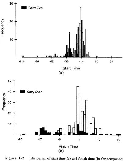
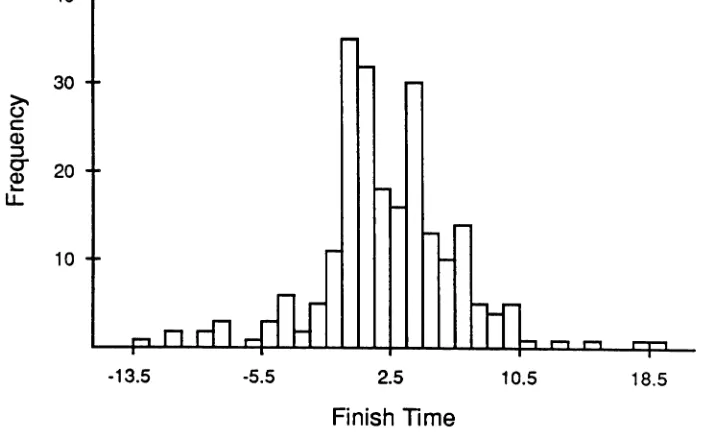
Histograms of the start and finish times for components in Project 1 are shown in Figure
1-2. Both distributions ofnew components have approximately normal, or Gaussian,
CCSP-lR-91/19/Modeling Behaviorof Large SoftwareProjects/NCSU.CSC/DSB .MAVIJune-1991 7
30
- CarryOver
>-20
o
c:
Q)
:J
cr
Q)
~
U. 10
-110 -86 -62 -38 -14 10 34
50
40
>-o
c:
Q)
:J 30 CJ ~
u..
20
_ CarryOver
Start Time (a)
10
-26 -17 -8
Finish Time
(b)
10 19
Figure 1-2
Histogram of start time (a) and finish time (b) for components in Project 1.ccsr-
TR-91/19/Modeling Behavior of Large Software Projects/NCSU.CSC/DSB.MAVIJune-1991 8distribution. Of interest is the probability that a certain percentage of product components will finish by a certain time. The model described in this study can be used to project and estimate the cumulative frequency curve.
300
•
Carry Over Programs• New Programs
~ Sum
c
c:
0> 200
::J
C-O>
~
u,
0>
>
:;=
as 100
's E
::J
o
0
-25 -20 -1 5 -1 0 -5 0 5 1 0 1 5 20
Finish Time
Figure 1-3 Cumulative frequency plot for component finish times for com-ponents in Project 1. The comcom-ponents are partitioned according to their classification as new or carried over, as discussed esrlier.
It was determined that a linear, additive regression model provides an adequate description of the component phase durations (and therefore finish) behavior. In this case, the model used component start time as the predictor variable and component phase duration as the response variable. Ingeneral, regression provides a model where the mean level of the response variable can be estimated as a function of one or more predictor variables. The level of confidence depends on the variance of the response variable about its expected value, given by a regression function. Also necessary for confidence interval statements
and hypothesis testing is the normality of the random error term in the regression model.
Using regression diagnostics, it was determined that this assumption is not grossly invalid
CCSP-1R-91/19/Modeling Behaviorof Large SoftwareProjects/NCSU.CSC/DSB.MAV/June-1991 9
For reasons of simplicity, the predictor variable selection was limited to a single quantitative variable: component phase starting time. Other quantitative independent variables may prove significant in other environments, although not necessarily in a linear and/or additive fashion. A measure of lines of code could be used as an additional quantitative variable. Also, qualitative variables may prove useful inreducing variability in the observed dependent variable. Qualitative variables can be incorporated into regression models in the form of
class variables
(e.g., [Rawlings, 1988], esp. chapter 8). Managers, departments and program type are examples of possible qualitative variables.1.3 Review of Past Work
This section briefly discusses some existing software schedule estimation models. The concepts behind Parkinson's Law and the Deadline Effect, which are important to this model, are defmed and discussed
1.3.1 Software Schedule Estimation Models
ccsP..TR..
91/19/Modeling Behavior of Large Software Projects/NCSU.CSC/DSB.MAV
/June-1991 10On the other hand, macro-estimation is most applicable to large systems. Estimates are
made at theproductlevel, and not at the individual component level. Initial estimates for
the product are used early in the project life-cycle in order to predict the manloading
(number of staff required at any given time) and the schedule. An example of a
macro-estimation model for software systems is Lawrence Putnam's SLIM
[Putnam-Fitzsimmons, 1979]. The form of the Putnam model is
S, = CkK l(31:d4/3
where S,is the number of lines of delivered source code, Ck is a constant (called the "state
of technology" constant),
t<I
is the development time in years, andKis the life cycle effort in man-years. As can be seen, the model relates the size of the product to the effort and time required to develop it. The effort and the development time can be related moregenerally by
Effort
=
c /1d4where Effort is
an
estimate of effort in man-years, and c is a constant in the range 14 to 15 [Boehm, 1981].The
COCOMO
model [Boehm, 1981] is another example of a macro-estimation model. It relates the size of the product to the required effort and the development time. TheCOCOMO
model isan
example of a more general set of multiplicitive models. This type ofmodel estimates the effortwithequations of the form
Effort
=
aXbwhere a and b are constants, and X is a measure of product size. The models estimate
development time withequations of the form
CCSP-TR-91/19/Modeling Behavior of Large Software Projects/NCSU.CSC/DSB.MAV/June-1991 11
where c and d are constants, and Effort is an estimate of the effort. Surveys of several
models of this type can be found in [Boehm, 1981] or [Fairley, 1985].
The COCOMO model is flexible because it can utilize added information and become a
micro-estimation tool. COCOMO can be thought of as a micro-estimation tool in its
intermediateand detailed forms.
Macro models like the Putnam and basic COCOMO models are macro in the sense of the
product and the time interval considered. Product-level estimates are used to estimate the
nominaleffort and calendar time (schedule) required to develop the product. However,
COCOMO can be used as a micro-model, to "focus in" on both the product and the time
intervals. A shortcoming of macro-estimation techniques, as explained by Boehm, is that
they assume that the (cost) driving factors are applied equally throughout the entire
life-cycle and the product (e.g., thatall the personnel are equally qualified and motivated, the product components are of similar complexity, and so on).
1.3.2 Parkinson's Law and the Deadline Effect
Software developers spend their time on many things, and they divide it up among the
activities they must perform. Suppose a developer (or a team of developers) reports he
started an activity of interest, A, at time 0 and finished at time 5. However, what he fails to
report is that he worked on activity B, which is unrelated to the completion of activity A,
from time 2 to time 3, at which time he was not working on activity A. An activity duration
of 5 units is reported, when only 4 units were needed to finish activity A. The
unpredictability of the partitioning of the developer's time contributes to the randomness of
cess-
TR-91/19/Modeling Behavior of Large SoftwareProjects/NCSU.CSC/DSB.MAV/June-1991 12if the activities "belong" to different projects. An illustration of a partitioning of total reported activity time appears belowt,
1:::::,::::1
=Time spent on other activitiesD
=Time spent on activity AFigure 1-4 . Example of a partition of a software developer's time.
Parkinson's Law states that work will expand to fill the allocated time. This may occur because of an overestimate of the time needed for the project, or by activity time mis-management on the part of the developers. Developer behavior could be affected by the knowledge of the planned milestone date. The programs that start (i.e., begin a life-cycle phase) closer to the planned milestone date take less time to complete than those that start further away. That is, the completion duration becomes more or less the amount of time that was originally available until the milestone date. Hence, it may happen that the same program will require different amounts of time to finish a phase, depending on how close to the due date work on it commences.
['m not sure the next couple weeks would be valid [for an effort study
J.
We are in our normal...panic to meet a key ...milestone. This is not the norm and I think the study would not be valid based on the next couple weeks...The above comment is an excerpt from a reply to a call for volunteers to participate in an effort study. Several software managers were asked to participate in the study. The replies varied, but they earned two common themes: 1) "What's in it for us?" and 2) "This is the worst time for it". The first question is certainly valid, and one answer is: improvement in the planning and control of the software development process so thatit is possible to bring a quality software product to market on schedule and within budget. The second theme is
CCSP-lR-91/19/Modeling Behaviorof Large SoftwareProjects/NCSU.CSC/DSB.MAVIJune-1991 13
intriguing. Why are the few weeks before a major milestone date so different from the rest, or "the worst time for it"? It's called the Deadline Effect:
The amount of energyand effortdevoted to an activityis strongly acceleratedas one approachesthedeadline for completing the activity. [Boehm, 1981]
Sometimes software developers increase their effort closer to the milestone date in order to make the deadline. The Deadline Effect is loosely the converse of Parkinson's Law. Suppose a developer believes he cannot make a deadline by working at his present pace. He then puts in the extra effort (in the form of overtime, skipping lunch, etc.) to finish his activity by the due date. The time needed to complete the activity thus becomes the time that was allotted. Note that the extra effort the developer has put into the activity, by "borrowing" time from his other activities, is often not recorded in the reported development time.
As Parkinson's Law and the Deadline Effect suggest, the actual placement of milestone dates can have an impact on the time and effort devoted to activities (and therefore to their fmish times). The impact, in some cases, causes planned milestone dates to become "self-fulfilling prophecies'". Parkinson's Law and the Deadline Effect may be common to many software development environments, which shall becalledmilestone date-driven.
Based on the previous discussion, it could be assumed that not all components in a project finish early, even if the schedule is relaxed. Rather, a significant number of them may finish on time at best. The key point here is that a developer's perception of the time allotted partly governs the time and effort he puts forth to achieve a milestone. This effort, and therefore the development time of the components, depends on the placement of milestone dates. Of course, software managers are not free to arbitrarily place milestones
CCSP-TR-91/19/Modeling Behavior of Large Software Projects/NCSU.CSC/DSB.MAV/June-1991 14
dates to speed up the overall process. For example, Boehm reports that schedules typically
cannot be compressed to less than 75% of the nominal schedule [Boehm, 1981]. Milestone
date placement requires a good understanding of the software product and the process, as
well as a good prediction of how long the project and its individual components should take
to complete. Any of the methods mentioned earlier (i.e., the Putnam or COCOMO models)
can and should be used to estimate such quantities.
Simply scheduling the components of a projectin a certain way could also lead to the self-fulfilling prophecy effect. For example, large programs will usually be given more time
than the small ones, and so they willbe started earlier, with the hope that theyallwill finish by the time the project is planned tobefinished. We are not asserting that all programs will
finish at the same time, on the due date, but rather that developers will tend to manage their
time in such a way so as to finish as near to the due date as possible.
1. 4 Scope of this Study
The focus of this study is on providing a regression model to describe the behavior of
software projects developed under a phased, milestone date-driven software development
process. The model is a stochastic macro-model. It describes behavior at the product
level, but uses stochastic component-level information to arrive at the description. The
basic assumption is that a schedule for the project is set, and that its planned milestone
dates are known to all the staff working on the project. The planned milestone date of a
life-cycle phasewillbe related to the duration of the components for that phase.
The model is a macro model at the product level, but it is a micro-model at the time level.
The product is viewed as a collection of software components which behave in a stochastic
CCSP-TR-91/19/Modeling Behaviorof Large SoftwareProjects/NCSU.CSC/DSB.MAV/June-1991 15
time, and therefore to the time at which developers finish any given life-cycle phase. The
model can be applied to any of the life-cycle phases, or to any combination of adjacent
phases.
To illustrate the model, a linear, additive model is defined. Least squares regression is
used to estimate the model parameters. For each product component, the expected phase
duration is expresseda~a function of one predictor variable: start time relative to the phase
milestone date:
Duration
=
a+
bXwhere X is the start time and a and b are constants. Other predictor variables could be
identified and incorporated.
Parkinson's Law and the Deadline Effect will be quantified by assuming that the average
time required to complete a phase will be the time that has been allotted. Once a schedule
has been set, and a date chosen for the projectcompletion, the model derived in this study can be used to describe the average behavior of the product components (provided they
follow a development process similar to the one described in this study).
1. 5 Overview of the Study
Section 2 covers the development and derivation of the model. Section 2.1 enumerates and
discusses the definitions and assumptions of the model. A detailed description of the
software environment is presented in Section 2.2. Section 2.3 contains the model
development. Section 2.3.1 lays the groundwork for the model with notation and
definitions. A description of the distribution of finish times is derived in Section 2.3.2. The expectations of program durations and finish times are discussed in Section 2.3.3.
CCSP-TR-91/19/Modeling Behavior of Large Software Projects/NCSU.CSC/DSB .MAVIIune-1991 16
defmes the model as a linear additive model. Formulas for estimating the variances of durations and fmish times are given in Section 2.3.5. The model's implications with respect to schedule changes are consideredin Section 2.4.
Section 3 contains an evaluation of the model. Both simulated and empirical data were used to evaluate the model. The model's performance on simulated component/project data in the absence of schedule changes is observed in Section 3.1.1. The effect of schedule changes on the project behavior is simulated in Section 3.1.2. The results of empirical data analyses are presented in Section 3.2.
CCSP-lR-91/19/Modeling Behavior of Large Software Projects/NCSU.CSC/DSB.MAV/June-1991 17
2
MODEL DEVELOPMENT
The observations presented in Section 1.2 suggest that there is a relationship between the
component starting time and its duration for a given life-cycle phase. It appears that the
components that start closer to the planned milestone date for a phase will require less time
to complete that phase than those that start further away. Although we cannot assert that
observations from the present data guarantee a causal relationship, the dependence of
program duration on its starting time relative to the milestone date seems reasonable. The
dependence is suggested by Parkinson's Law and the Deadline Effect.
2.1 Model Definitions and Assumptions
Most terms usedin this report have widely accepted meanings and are generally used in a broader context. More specific definitions are adopted in order to avoid ambiguity. The
model can be expanded for use with broader definitionst.
DEFINITIONS
• A software product is a package of two or more deliverables. Products are
sometimes called software systems.
• A deliverable is software: a program and/or supporting documentation.
Deliverables were also called components in earlier discussions. Aprogramis a
collection of instructions that can be run on a computer. Throughout the report,
however, program will be used as a synonym for deliverable or component.
• Every software project is governed by aprocess, which includes the full set of
activities necessary to deliver the software product, including a particular
life-cycle model.
CCSP-TR-91/19/Modeling Behaviorof Large SoftwareProjects/NCSU.CSC/DSB.MAVIIune-1991 18
• A softwareprojectdefines the mapping between the software process and the
software product. Every product is different, and requires a different mapping to
the process.
• A milestone date is a point in time that serves as a goal for software product
developers. The goal is the completion of certain deliverables, at which time the
milestoneis achieved.
• Milestones can be eitherhardorsoft. The difference between the two types lies
in the criteria required to achieve the milestone. The criteria required for a hard
milestone are measurable and verifiable, like the completion of a detailed design
document that has been approved by the developer's manager(s) and peers. To
achieve the milestone, the criteria are enforced. The criteria required for a soft
milestone may be ambiguous, can lead to confusion, and usually do not entail
verification of deliverables.
• A project's life cycle is divided into phases. A program start time is the time at
which the program begins a life-cycle phase. A programfinish timeis the time at
which the program completes the same life-cycle phase. Both times will be
measured with respect to a planned, fixed milestone date for that phase.
• A programphase duration, or justduration, is
us
finish timeminus itsstart time.In this report, all starting and finishing times for a life-cycle phase are scaled to preserve the
time measurements across multiple projects. First, all the program start, finish times and
project milestone dates are converted to an appropriate linear scale (e.g. Julian dates). The
planned finish milestone date for the phase is subtracted from the starting and finishing
times, and from the milestone dates. This scaling provides adistance to milestone date
measure. Durations are measured in the same units as the scaled dates (e.g., days). The
scaling technique also provides a basis for measuring the evolution of project schedules,
CCSP-TR-91/19/Modeling Behavior of Large Software Projects/NCSU.CSC/DSB.MAVIIune-1991 19
The definitions of start time and finish time apply to any life-cycle phase. For reasons of
simplicity, the phase discussed in this paper is the design and coding phase. This phase is defined to begin at the start of high-level design and end at the completion of coding, unit testing and integration. The relationships observed for this phase have also been observed for other phases (e.g., specification to system test completion). The relationships tend to be stronger (i.e., show stronger correlation) when the phase milestone is a hard milestone. This is discussed in more detail below.
ASSUMPTIONS
1) Program durations behave as random variables.
This assumption allows the phase durations tobeviewed as samples from populations that couldbe described by probability distributions. The assumption also permits the application of probability theory in order to make inferences. The information that is relied on the most, the reported start and fmish times of a program development activity, is usually incomplete. That is, the duration reported for an activity is not
necessarily an accurate measure of the time spent solely on that activity. The idea of the »npredictable nature of the time spent on activities was addressed earlier, in Section 1.3.2.
There may be a problem in the reporting of the times itself. If the developers are responsible for reporting their own times, they may report that a program has achieved a milestone when it has not, or they may finish the program, but not report that it is finished until the due date. The first kind of reporting error may occur because the developer interprets the status of his activity differently than his manager. The second type of error might be caused by simple negligence, or it might be partly caused by a misunderstanding of the value of accurate information.
Some of the problems linked to reporting can be associated with the milestones used in the schedule. If milestones are hard, or well-defined and measurable, there should be
little disagreement between the managers and the developers about the status of an activity. The requirements for completion of a milestone are spelled out explicitly, and must be met unconditionally. If the milestones are soft, then opinions can determine
CCSP-TR-91/19/Modeling Behavior of Large Software Projects/NCSU.CSC/DSB.MAV/June-1991 20
should be avoided, or at least be kept off the critical pathin the project schedule. Truly
not achieving soft milestones on time should not lead to a change in the final milestone
date, if it can be avoided [Brooks, 1975]. By defmition, soft milestones are associated
with confusion, and one would like to be as definitive as possible about the finish date.
Note For the model, observations on the predictor variable (i.e., reported component start time) are considered to be known constants. This means thatreported data are
correct, and it is this reported data that will be used to build the model (see Section 2.2).
2) Program durations are independent of each other.
This assumption will always be violated somewhat in real software projects. For
example, product components are interdependent during integration and integration
testing. The assumption does, however, allow us to further simplify the derivation of
model formulas.
3) Expected program duration is, on average, equal to the time remaining to the planned milestone date.
This assumption forms the basis of the linear modeling approach, which is used to
demonstrate the model. Expected program duration is assumed to decrease as program
starting time approaches the planned milestone date. This means that, on average,
programs that start closer to the planned milestone date will require less time to finish a
life-cycle phase than those that start further away. Variation in the duration for
programs starting at the same timewill be caused by differing program attributes and
development conditions. These attributes could perhaps be incorporated into a more
CCSP-TR-91/19/Modeling Behavior of Large Software Projects/NCSU.CSC/DSB.MAV/June-1991 21
4) Deviations of program duration about their expected value are normally distributed with mean O.
It is also assumed
4a) Deviations have common variance, (12, across all values of the
predictor variable, and
4b) Deviations are independent.
These are typical assumptions madein least squares regression. These assumptions do not seem to be artificial, based on regression diagnostics of historical data. The assumption also implies that the program durations are normally distributed about their expected value with common variance. Under the normality assumption, the least squares estimates are equal to the maximum likelihood estimates. For more on maximum likelihood estimation, see [Rawlings, 1988] or [Searle, 1971]. Assuming the deviations are normally distributed also provides the basis for hypothesis testing and confidence interval statements, but is not necessary to estimate by least squares.
Discussion Under the assumptions, which assume a process, the behavior of a software project canbe described. The behavior is described in terms of the product components, the programs. During a phase, the development of a single program is an activity. The reported time required for an activity is considered to be a known instance of a random variable. The reported times include the time spent on other activities. The assumptions imply that developers will manage their time so that the activities they are responsible for take time approximately equal to the amount of time they are given. Variationsin activity difficulty, individual developer ability, and the way developers manage their time cause the variations in activity durations. Inother words, it is assumed that developers will "aim" for the due date (on average), and they will miss it with an error which is normally distributed.
CCSP-TR-91/19/Modeling Behaviorof Large Software Projects/NCSU.CSC/DSB.MAVIJune-199l 22
programs that start at very different times may have similar chancesoifintshing on time, but they will have very different durations. For this reason, duration is used as the dependent variable (rather than finish time). One could then focus on program attributes that affect duration for a given phase. Such attributes can possibly be used as variance-reduction factors. A measure of complexity serves as an example: iftwo programs start on the same day, and the first is quite simple and the second very complex, then they will likely take different amounts of time to design, implement and test
2. 2 Detailed Description of the Development
Environment
An important part of the model development is the environment that contains the projects. This section elaborates on the attributes of the environmentin which the model operates. The software development environment described here has practical value, in the sense that it, or its variants, is being usedinindustry on large software projects.
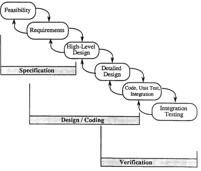
Software projects combine products and a process. The observed process life-cycle resembles the classic waterfall model (see [Boehm, 1981] or [Pressman, 1988]). The entire software development is divided into phases separated by milestones, or goals, to be attained at the end of each phase. Each program that makes up a software product follows the same life-cycle model, which is similar to that of the entire product. When a predetermined fraction of programs achieve a given milestone, then the product is said to have achieved that milestone. Inorder to deliver the completed product, all programs that remain in the product must achieve the [mal milestone. Any programs that do not must be abandoned, and perhaps re-instated at a later time, as part of another product release,
during another project. It is not necessary that all program development starts at the same
time. Also, it is not expected that all programs will achieve intermediate or the final
CCSP-TR-91/19/Modeling Behavior of Large Software Projects/NCSU.CSC/DSB.MAVIJune-1991 23
The integration and system testing is typically performed by a separate group of people from those who designed, unit tested and integrated the software. However, there is contact between the independent testers and designers. Recall that the modeling approach willbeillustrated for the design and coding phase, which begins with high-level design and ends after coding, unit testing and integration.
The entire development life-cycle model is illustrated in more detail in Figure 2-1. The project proceeds from left to right, but it can backtrack, if needed. Reasons for backtracking (or feedback) include re-work on design because of an error that was discovered, or by a changeinrequirements. Backtracking is not limited to one phase.
cess-
TR -9 1/19/Modeling Behavior of Large Software Projects/NCSU.CSC/DSB .MA VIJune-1991 24DESCRIPTION OF THE LIFE-CYCLE PHASES
Specification: During the specification portion of the development, the major commercial functions of the product are defined. Also, efforts are made to assess
the feasibility, content, and size of the product. Project plans are created in this
stage to define the progression of the process. The specification phase contains
three subphases:
• Feasibility
Program specification documents are written during the feasibility phase.
In order to complete the phase,allrequired specification documents must be completed.
• Requirements
The requirements phase focuses on planning development and finalizing
requirements. Preliminary project schedules are drawn up, requirements
are mapped onto development activities, and staffing is arranged. At this
stage, the individual activities are usually (and should be) entered into an
online database in order to track their development status.
• High-Level Design
Detailed functional specifications are reviewed and finalized in this phase.
Also finalized are development plans, including release priority,
packaging, and schedules.
Design / Coding: Once the specifications are finalized, the development of the
software to implement their functions is begun. The design / coding phase
includes high-level and detailed design, and unit testing. It consists of two
subphases:
• Detailed product design
The design of the programs is performed in this phase. First, a high-level
design breaks the program down into small modules and their architecture
is developed. A detailed design of each module follows. To complete the
phase, the high-level and detailed design documents must be completed,
CCSP-TR-91/19/Modeling Behavior of LargeSoftware Projects/NCSU.CSC/DSB.MAVIJune-1991 25
• Code, unit test and integration
During this phase, program modules are implemented. Each programmer
tests his modules with help from an independent tester. To complete the
phase, the code must be inspected and tested by the designer, analyzed
using code coverage tools, and placed under change control in a code
library.
Verification: The verification phase focuses on regression and traffic testing (which simulates actual operational environments) of the existing software base,
in order to ensure that it is not corrupted by any new software development.
• Integration testing
Established performance metrics related to failure rates must be satisfied
before this phase is completed. The testing at this stage is at the product
level (i.e., all the programs in the product have been coded, unit tested
and integrated).
It is possible for more than one project to be underway at a time. Product developers
divide their time among several projects. Each project applies the same life-cycle model
(process), discussed above. The projects overlap in their different phases. For example,
system testinginprojectN-l may overlap design in project N and specification in project N+ 1. The goal of each project is to deliver an enhanced version of the software product,
the next release. Work on the enhanced version of the software includes updates (including
error corrections) to existing software as well as additions. Project planning may be
simplified somewhatbythe repetitive nature of the process and similarities in component
functionality. An illustration of the overlapping nature of the projects is shown in Figure
CCSP-TR-91/19/Modeling Behavior of Large Software Projects/NCSU.CSC/DSB .MAV/June-1991 26
Product Released
Time ~
)~
)
) ~" ,
"~
I
Project N-1I
Project NI
Project N+1CCSP-TR-91/19/Modeling Behaviorof Large Software Projects/NCSU.CSC/DSB.MAVIJune-1991 27
2.3 The Single-Variable Model
In this Section, the model is expressed in terms of a regression function. A linear
regression function is used to demonstrate themodel,
2.3.1 Model Notation and Definitions
Capital letters are used to indicate random variables. For example: X. Lower case letters
indicate a specific realization, or instance, of a random variable. For example,Xexmeans
"the random variable X has taken the value x". A random variable that is conditioned on
another will be written as Yx ,where Y is conditioned on X=x. The notation "YIX=x", or
"Y Ix" means "Y, given Xex", and is sometimes used, also. The distinction between the
subscripted and non-subscripted variables is that the subscripted variables imply
dependence. For example, Y denotes any random program duration, independent of start
time; Yxdenotes a random duration for agiven start time, X=x.
Definition Let X be program start timet, Y be program duration and Z
=
X + Y beprogram finish time. Let Yx be program duration for a program starting at time X=x, and
letZx = x+Yxbethe program finish time for a program starting at time X=x.
Definition Let X and Y be discrete random variables having joint probability mass
function (pmf) p(x,y). Theconditional pmf of Y given X, is
PYlx(ylx) = P(y=yI X = x) = P(y = y, X = x) = p(x,y)
P(X = x) px(x)
where Px(x)~O. [Trivedi, 1982]
t Recall from Section2.1that"times"referstoreportedtimes.
cess.
TR-91/19/Modeling Behavior of Large Software Projects/NCSU.CSC/DSB .MAV/June-1991 28Definition Let D(x) = E[Z I X=x] be the regression function for duration on start time. D(x) is the expected duration for a program starting at time X=x. The theorem of total
expectation for anydiscrete random variables X and Y states
E[Y] =
L
E[YIX=x]px(x) =L
D(x)px(x)x x
[Trivedi, 1982, esp. chapter 5]
(2.2)
This formula shows how to calculate the unconditional expectation of Y, given the
regression function, D(x) and the pmf for X.
2.3.2 Calculating the Distribution of Finish Times
In this section, the start time distribution and the conditional duration distributions are related to the finish time distribution. Distributions of durations for a given starting time are represented by conditional distributions.
Using the definitionsin Section 2.3.1, it follows that the pmf, Pz(z), for all program finish times, Z= X+Y, can bederived as:
z
P(Z=z) =
L
P(X = x, X+Y
=z)
x--
z=
L
P(X
=
x, Y
=
z-x)
x--z
=
L
PYIX(Z-XI
x) PX(x)x--
(2.3)
The last line follows from the definition of conditional pmf. Note that this distribution describes the probability that any program that starts will finish at time z. It takes into
ccsr-
TR-91/19/Modeling Behavior of Large Software Projects/NCSU.CSC/DSB.MAVIJune-1991 29negative, which fits the model nicely, but extra care must be taken when trying to apply the
above formula to real situations. For example, when linear least squares regression is
applied in Section 2.3.3, it may be the case that the model predicts a negativeyvalue (near
the planned milestone date, 0, on Figure 2-3).
We can also calculate the probability that a program will finish at time z, given that it has
begun at timeXQ. The. answer is simply PYlx(Y=z-xOIX=xO). Given that a program starts
at time XQ,there is only one value ofythat, when added to xo, gives z. This value is, of
course, y= z-xo.
Let pz(t) be the pmf of finish times, and let
Fz(t)=
L
pz(z)zSt
(2.4)
be the cumulative distribution of finish times. Suppose there are N programsin the project. Then, the expected number of programs that will be fmished by time
to
is N · Fz(to).2.3.3 The Expected Values of Durations and Finish Times
Inthis section, the formula for the expectation for all program durations is derived. Recall
that Y =program duration. It follows by the theorem of total expectation (equation 2.2)
that, for all programs, the expected duration is
E(Y]
=
L
Px(x) E[Ylx]=
L
Px(x) D(x)x x
(2.5)
In the case where D(x) is a linear function of x, equation 2.5 can be reduced to E[Y] =
D(E[X]).
CCSP-lR-91/19/Modeling Behavior of Large Software Projects/NCSU.CSC/DSB .MAV/1une-1991 30
E[ZxoJ
=
E[xQ+YxoJ
=
E[xQ]+ E[Yxo]
=
xQ + D(xQ) (2.6)Using the rules of expected value and Equation 2.5 above, we can derive the expected
finish time Z
=
X+
Y, of all programs byE[Z]
=
E[X +y]=
E[X] +E[Y] (2.7)Equation 2.7 can also be derived using the theorem of total expectation, bysumming over all possible values of x, the expression for E[ZxJ times Px(x). Inthe case whereD(x) is a
linear function of x, equation 2.7 can be reduced to E[Z]
=
E[X] +D(E[X]).2.3.4 Applying Least Squares Linear Regression
The assumptions listed in Section 2.1 suggest least squares linear regression canbeapplied to estimate the parameters in the relationship between program start time relative to the
planned milestone date and duration.
::.tlppose the relationship between starting time and expected duration be linear, as is
suggested by the observations presented in Section 1.2. Then, we can expect a relationship
CCSP-TR-91/19/Modeling Behaviorof Large Software Projects/NCSU.CSC/DSB.MAVIJune-1991 31
Duration
Start Time, x
(relative to milestone)
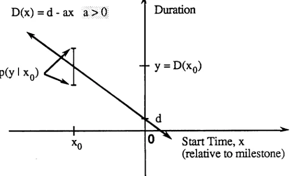
Figure 2-3 Defined linear relationship between program starting time and duration. A conditional distribution, PYIX(y1XO), of durations for a given starting time, XQ, is shown.
Observe that start times have been emphasized as being negative. The definition of start time requires the subtraction of a program's start time and the planned milestone date (see Section2.1).
Figure 2-3 clearly indicates that a program that starts closer to the planned milestone date will require less time to finish than one that starts further away from the milestone. Of course, this behavior cannot be expected to carry on right up to the milestone date in reality, since all programs have some certain minimum development time. However, for programs that start very close to, or beyond the planned milestone, it will be assumed that the linear relationship holds, owing to the Deadline Effect. This should rarely be observed, since programs are usually started before the planned milestone date.
ccsr-
TR-91/19/Modeling Behavior of Large Software Projects/NCSU.CSC/DSB.MAV/June-1991 32including the developer and complexity. On the basis of historical data analysis,
probability distributions could be assigned to suit a particular development environment.
For this model, assumptions have been made about the duration distributions for a fixed
start time in order to conform to least squares regression model (i.e., for hypothesis testing
and confidence interval statements). Figure 2-3 also illustrates the idea of the consideration
of a distribution of durations for a given start time. These distributions can thought of as
conditional distributions, with the conditioning being on start time.
THE SLOPE OF THE REGRESSION LINE
Assuming the linear relationship exists, what is its expected behavior? Should it have slope
-2, or -1/2, and what should the intercept be? Suppose the work on a given program expanded to fillthe allotted time, or that it was accelerated to finish on time (assumption 3,
Section 2.1). Then, on average, the development time would be equal to the allotted time.
Therefore, the slope of the line in Figure 2-3 should be -1, since the time needed for
development (duration) is the time allotted (start time, relative to the planned milestone
date).
If the planned milestone date must be changed to a new date for any reason, the model
changes. This illustrates the proposed dependence of program development time on
milestone placement. The developers working on programs that have not finished by the time the milestone date is changed are now targeting a new date. The idea of schedule
changes is discussed further in section 2.4, and is simulated in Section 3.1.2.
Let
Yi
=
80+8lXi +Eiwhere
Eiis a
randomerror
termwith
mean O.CCSP-1R-91/19/Modeling Behavior of Large Software Projects/NCSU.CSC/DSB.MAV/June-1991 33
This is a common definition of a linear regression model with one independent quantitative variable. 80 is the intercept term and 81 is the slope of the regression line. Yiis an observation on the dependent variable, phase duration, and Xiis an observation on the independent variable, phase start time.
The method of least squares gives the best linear unbiased estimators of 80 and 81. They
1\ 1\
are best in the sense that they have minimum variance among all estimators. If Bo and 31
"
"
"
are estimates for BO and 81,respectively, then Yi= BO +81Xiis an estimator for E[yiJ = 30
+81Xi [Rawlings, 1988].
The interpretation of the line, from Figure 2-3, is that D(x) =E[yIX=x],or that for a given starting time, x, the expected duration is D(x). The conditional expected value of a program duration is thus a linear function of the expected value of the start time associated
1\
with it. D(x) is the regression function of duration on start time. We therefore use 80to
1\ 1\
estimate d, the intercept. Similarly, we use81 to estimate a. Note that a ~ 0, so -81 will estimate a.
Assumption 4 in Section 2.1 states that the random errors,Ei,are normally distributed with equal variance. This assumption provides the basis for confidence interval statements and
1\ 1\
CCSP-TR-91/19/Modeling Behavior of Large Software Projects/NCSU.CSC/DSB.MAV/June-1991 34
2.3.5 Estimating the Variances of Duration and Finish Times
Under the assumption that the random errors, Ei, are normally distributed with equal
variance, y1, ... ,YN also have independent, normal distribudons". Furthermore, the true
variance of duration, YXa' for a given start time ofxo,is equal to the variance of the error,
A
a
2 . Leta
2be the mean square error from thefitFor a given value of the independent variable, xo, the estimated variance of the mean
responseinthe dependent variable is
a
2[_1
+-=-(XO_-__X)~2
]N
~(xj-xl
1
(2.9)
Also, for a value of the independent variable, Xnew, the variance of the prediction of
dependent variable,Ypred-is
(2.10)
Recall that the probability that a program will finish at time z, given that it has started at
time
xo,
is PYIX(Y=z-xoIX=xo).
It follows that the variance of the estimated expected finish time, for a fixed starting time XQis givenbyequation 2.9. Similarly, the variance ofpredictedfmish time for a fixedstartingtime X()isgivenbyequation 2.10 above.
CCSP-TR-91/19/Modeling Behavior of Large Software Projects/NCSU.CSC/DSB.MAV/June-1991 35
2. 4 The Effect of Schedule Changes
Schedule "slippage" dominates the history of software development project schedules. The slippage is generally caused by a tendency to underestimate the time needed to complete a project. Some of the reasons for the underestimates are listed in [Fairley, 1985]. Fairley summarized a Bell Labs time and motion study of70programmers conducted by Bairdain in 1964. The study revealed how programmers typically spend their time. Surprisingly, only 13 percent of programmers' time was spent on writing programs! The rest of their time was spent on:
Reading programs and manuals Job communication
Personal Miscellaneous Training
16%
32% 13% 15%
6%
5% (Bell Labs, 1964)
Therefore, Fairley reports that a major reason for underestimating software project schedules is failing to account for the 13+ 15+6+ 5= 39 percent overhead time for the programmers and the 16
+
32=
48 percent overhead time for job communication and reading of manuals and programs. Such schedule underestimates will lead to schedule changes.Only schedule changes that require a change in the milestone date willbeaddressed. Thus, schedule change will mean a change in the finish milestone date. Schedule changes do not necessarily require a change in the modeling approach. A changein a schedule only affects the progress on programs that remain unfinished at the time the change is announced. It will be assumed that the developers view the new due date (milestone date) as they viewed
the previous one. More on this can be found in section 3.1.2, where a simulation is run
ccsP-TR-91/19/Modeling Behavior of Large Software Projects/NCSU.CSC/DSB.MAV/June-1991 36
When a schedule slip is announced, how do the developers react? Obviously, the progress
on programs that have already finished by the time of the announcement (what we call the
slip date) will not be affected. For any programs that have not yet begun by the slip date,
one could assume that their developers view the new milestone date as they would view
any other. That is, the developers will tend to take the allotted time and finish the program
near to the (new) due date. So, the main focus is on those programs that began prior to the
slip date and did not finish by that time. One could argue that developers will fill their
remaining time (i.e., the time from the slip date to the new milestone), too, for reasons
similar to why they fill the entire interval. Other reasons for this behavior include:
• The developer could never have fmished by the old due date, and he needs the
extra time to finish. This reason, if it is widespread, may have actually motivated
the decision to slip the schedule.
• The developer could use the extra time to fulfill the specifications more
completely.
• The developer could fill the extra time by adding "bells and whistles" to the
program.
• The developer may spend more time performing unit testing.
• The developer might use the extra time to work on "slack time" activities, like
reading mail, training,personal activities, or working on another project. A more
detailed account is given in [Boehm, 1981].
Some of these possibilities were addressed before, when Parkinson's Law and the
Deadline Effect were discussed. Inthis report, it is assumed that the developers will indeed
filltheextra time:
Ifa k-unit schedule slip occurs at time t, expected phase durations of programs