ABSTRACT
VUTHA, ASHWIN KUMAR. A Microfluidic Device for Thermal Flow Cytometry. (Under the direction of Dr. Glenn Walker and Dr. Clement Kleinstreuer).
A Microfluidic Device for Thermal Flow Cytometry
by
Ashwin Kumar Vutha
A thesis submitted to the Graduate Faculty of North Carolina State University
in partial fulfillment of the requirements for the degree of
Master of Science
Mechanical Engineering
Raleigh, North Carolina 2013
APPROVED BY:
_______________________________ ______________________________ Dr. Clement Kleinstreuer Dr. Glenn Walker
Committee Co-Chair Committee Co-Chair
BIOGRAPHY
ACKNOWLEDGMENTS
TABLE OF CONTENTS
LIST OF TABLES………... vii
LIST OF FIGURES………... viii
Chapter 1 Introduction………. 1
1.1 History of Flow Cytometry………. 1
1.2 Miniaturization of the Coulter Counter………... 5
1.3 Methods for Counting Particles in Microchannels……….. 8
1.4 Research Objectives and Novel Contributions……… 15
Chapter 2 Computational Model……….. 19
2.1 Theory……….. 19
2.2 Numerical Model………. 24
2.3 Computational Results………. 30
2.4 Numerical Accuracy of Computational Model ………... 38
Chapter 3 Material and Methods………... 39
3.1 General Device Schematic………... 39
3.2 Experimental Setup……….. 41
3.3 Microfabrication……….. 44
3.3.2 Fabrication of SU8 Master for PDMS Channels……….. 47
3.3.3 PDMS Molding………. 51
3.4 First Generation Devices………... 53
3.4.1 Circuit Used for First Generation Devices………... 56
3.5 Second Generation Devices………... 59
3.5.1 Circuit Used for Second Generation Devices…………... 60
3.6 Third Generation Devices……… 61
3.6.1 Circuit Used for Third Generation Devices……….. 62
3.7 Fourth Generation Devices……….. 62
3.8 Preparation of Sample and Flow Conditions………... 63
Chapter 4 Results and Discussion……… 65
4.1 Results with First, Second and Third Generation Devices…….. 65
4.2 Results with Water-Slugs……… 67
4.3 Results with Fourth Generation Devices………... 68
4.4 Discussion……… 70
Chapter 5 Conclusions………... 76
5.1 Limitations of TFC……….. 76
5.2 Future Direction………... 77
LIST OF TABLES
Table 1: Comparison of experimental and computational results obtained (∆T in K) at
different flow rates and for a simulated heat flux value 793 W/m2………. 35
Table 2: Soft baking: time and temperature settings for a range of photoresist
thicknesses……… 50
Table 3: Exposure and intensity settings for range of photoresist thicknesses………... 50
Table 4: Post-exposure baking: time and temperature settings for a range of photoresist thicknesses………. 51
LIST OF FIGURES
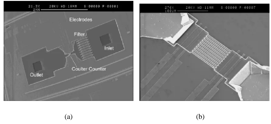
Figure 1.1: The Coulter Counter, developed by Wallace Coulter in the 1940s. The device was designed to allow the flow of a particulate suspension through a narrow orifice under a pressure head. The diameter of the orifice depends on the diameter of the particles to be counted. The description of the components indicated by the numbers can be found in (Coulter 1953, U.S Patent 2,656,508)... 3 Figure 1.2: Cross-sectional view of the channel without and with the presence of a particle (Coulter 1953, U.S Patent 2,656,508). With no particle, the gauge shows the constant value of the current supplied. For particles of different sizes, the gauge experiences different deflections... 4 Figure 1.3: The first microfluidic Coulter Counter developed (Larsen et. al 1997). Channels were fabricated by etching on a silicon substrate. Hydrodynamic focusing was applied by using a sheath fluid on either side of the sample. The electrodes were damaged during operation and therefore no repeatable results were possible... 6
Figure 1.6: (a) Schematic of impedance spectroscopy used to count and characterize cells (Gawad et. al 2001). The impedance measurement is made differentially between two pairs of electrodes, AC and BC. (b) The impedance signal obtained from (a) allows calculation of the speed of the particle... 10
Figure 1.7: Schematic for (a) Light-scattering particle counter and (b) Light-blocking particle counter (Zhang et al. 2009)………..…………... 12
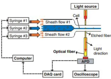
Figure 1.8: Schematic of the microfluidic flow cytometer based on fluorescence. Cells are hydrodynamically focused through the detection region. Light from the source is scattered by the cells and the APD converts the optical signals to electrical signals (Lin & Lee 2003)... 13
Figure 1.9: Schematic of the fluorescence-based device developed by (Cui et. al 2002). The light emitted from the particle has a longer wavelength than the incident light... 14
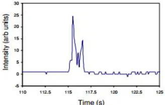
Figure 1.10: The intensity of light emitted from a 15 µm particle as detected by a light detector. (Cui et. al 2002)... 14
Figure 2.1: Geometry chosen for the computational model. The channel length and height were 8 mm and 250 µm respectively. The detection region (gray) was 180 µm long, between x=3 mm and x=3.18 mm. The particle (white) diameter was 90 µm. The red line at the bottom represents the heat flux applied as a rectangle function, which is described in section 2.2... 20
Figure 2.2: Bezier curves used to supplement the moving mesh. A in-built curve parameter 's' in COMSOL allows parametric conditions to be specified for the curves, which provide additional constraints that prevent inverted mesh elements……... 27
Figure 2.3: The 3D setup in COMSOL to determine the value of heat flux from the experiments. The square silicon nitride membrane of 300 µm side was at the bottom, the RTD above the membrane was 180 µm long, 20 µm wide and 200 nm high. The large block above the RTD is the volume of water that is in contact with the membrane at any given time... 29 Figure 2.4: The heat flux specified in the form of a rectangle function that goes to 1 between x=3 mm and x= 3.18 mm and 0 elsewhere………..….……... 29 Figure 2.5: Velocity profile for 90 µm particle with average fluid inlet velocity at 2 mm/s………..………... 30
Figure 2.8: Predicted temperature profile at chosen point for a 90 µm particle with fluid at 1.33 mm/s………...……... 32
Figure 2.9: Predicted temperature profile at chosen point for a 90 µm particle with fluid at 2 mm/s……….……..……... 33 Figure 2.10: Predicted temperature profile for a 90 µm particle with fluid at 2.66 mm/s……….……….………... 33 Figure 2.11: Comparison of the predicted signal at 1.33, 2 and 2.66 mm/s….…... 35
Figure 3.1: Schematic of the device used for TFC. A PDMS block with holes cored out was bonded to a substrate using oxygen plasma bonding…….……... 39 Figure 3.2: Block diagram for the experimental setup of TFC. In the final generation of devices, the circuit and data acquisition device were replaced by a multimeter…….... 41 Figure 3.3: Electrodes in the form of coils made by deposition of nickel on a glass substrate. A single coil is used for both heating and sensing. The other coil is provided for reusability of the substrate……….…... 42 Figure 3.4: The fixture used to hold the device in place during the experiments. The 'golden' pins at the center were the electrodes which made contact with the nickel deposited on the substrate of the device……….…………... 43
Figure 3.6: Process flow diagram for fabrication of glass substrates. AZ 5214 was used as a negative photoresist. Nickel was deposited to a height of ~ 200 nm using e-beam deposition………... 45
Figure 3.7: Process flow diagram for fabrication of SU8 masters. Source: (Dr. Glenn Walker)………..………... 47
Figure 3.8: Graph of photoresist film thickness obtained vs spin speed. Source: MicroChem………..…... 49
Figure 3.9: Representative channels fabricated in a PDMS mold. Blocks were cut out, each containing one channel, and bonded to a substrate. Red arrows point to the channels formed in the block………..…... 53 Figure 3.10: Early designs for the mask used in channel fabrication. (a) The angled channels were incorporated to allow hydrodynamic focusing of the solid particles. (b) The angled channels were replaced by a loop to reduce the number of syringes required... 54 Figure 3.11: Mask with T-junction channel included for testing the device using water-slugs. The channels in the first and second row are 1 mm wide. The channels in the third row are 0.3 mm wide. The remaining channels were not used………... 55
Figure 3.14: Block diagram of the first generation of the analog circuit that was constructed on a breadboard and connected to a data acquisition system (NI USB-6009)………... 57
Figure 3.15: Second generation of devices with the inlet tube eliminated and replaced with a large cored out vertical column that serves as a storage well for the suspension………..……... 59 Figure 3.16: Block diagram of the second generation of constant current circuits used. The additional instrumentation amplifiers from the first generation circuit were eliminated to prevent saturation of the circuit………... 60 Figure 3.17: Third generation of devices which differed from the second generation only in the orientation of the substrate. The substrate was flipped over so that the RTD was inside the channel………... 62 Figure 3.18: (top left) Silicon substrate patterned with nickel and (top right) magnified image of the sensor on the substrate. (bottom right) Diagram of enlarged sensor pattern. The width of the nickel strip was approximately 10 µm. (bottom left) 2D schematic of substrate... 63 Figure 4.1: MATLAB plot of voltage amplitude against time. The sharp peaks indicate the response to a disturbance introduced into the circuit by blowing air over it………...…... 66
Figure 4.3: Detection of DI water-slugs in the microchannel. The size of the slugs relative to the channel and the sensor, ensured distinct signals………...…..…... 68
Figure 4.4: 90 µm beads detected at (a) 12 µl/min (b) 9 µl/min and (c) 6 µl/min……….…...……... 69
Chapter 1
Introduction
1.1 History of Flow Cytometry
Andrew Moldovan was one of the first to suggest the use of dynamic fluid-particle suspensions for biological analysis (Shapiro 2003). His proposed apparatus was intended to be used to screen red blood cells or yeast cells as they passed through a thin capillary, under a microscope. The microscope was to be fitted with a photodetector, which would record the presence of a cell on the basis of light obscuration.
While it is uncertain whether Moldovan actually built a device for this purpose, it came to be known that the technique he suggested could be suitably adopted for such analysis. Moldovan's proposal laid the foundation for much of the later instrumentation for flow cytometry. In 1965, Kamentsky and Melamed tried to improve on Moldovan's idea through the use of a spectrophotometer that recorded the ultraviolet (UV) absorption and scattering of blue light by cells flowing past a microscope objective at speeds exceeding 500 cells/s. This was followed by Dittrich and Göhde in 1969, who developed a flow chamber that could generate histograms of fluorescence intensity, based on the fluorescence of the DNA of alcohol-fixed cells (Givan 2001).
Figure 1.1: The Coulter Counter, developed by Wallace Coulter in the 1940s. The device was designed to allow the flow of a particulate suspension through a narrow orifice under a pressure head. A voltage potential is applied across the orifice. As particles flow through, the electrical impedance across the orifice increases and results in a drop in measured current. The diameter of the orifice depends on the diameter of the particles to be counted. The description of the components indicated by the numbers can be found in (Coulter 1953, U.S Patent 2,656,508).
Assuming that the electrical conductivities of the fluid and the dissolved particles are different, the presence of a particle in the channel will form a temporary partial or complete obstruction to the flow of current and this will cause a sharp change in current for the duration that the particle is in the channel. This method can be applied to a suspension containing particles of different types as well as one containing suspended particles of the same type. One of the important considerations in the use of such a device is that the particles to be counted must remain suspended in the carrier fluid without settling. Additionally, the length of the conduit or channel must be as short as possible to avoid the presence of multiple particles in the channel at the same instant (or minimize coincidence). This concern is also to be addressed by means of the concentration of the mixture. Dilute solutions are better suited for evaluation than concentrated ones. Fig 1.2 shows the effect of presence of a particle on the signal recorded by a Coulter Counter.
1.2 Miniaturization of the Coulter Counter
Although the original Coulter Counter was and continues to be a reliable resource for particle counting, researchers in the recent past have realized that its benefits could be increased by miniaturizing it. A 'micro Coulter Counter', in addition to the existing features of the full-scale counter, would be portable, much less expensive and quicker in producing results. It would also consume considerably smaller amounts of the analyte and buffer. Advancements in the field of micro-electromechanical systems (MEMS) have greatly facilitated efforts to produce such miniature particle counters. MEMS-based Coulter Counters can be produced in batches and are easy to fabricate. It is also convenient to add more functionalities to existing designs. The materials involved are often inexpensive and easily available. Small-scale counters also enable parallelization, that is, connecting several microchannels in parallel for simultaneous analysis of multiple samples. Since they are inexpensive, these counters can be disposed after using them once for a counting task which reduces cross-contamination of samples.
Figure 1.3: The first microfluidic Coulter Counter developed (Larsen et. al 1997). Channels were fabricated by etching on a silicon substrate. Hydrodynamic focusing was applied by using a sheath fluid on either side of the sample. The electrodes were damaged during operation and therefore no repeatable results were possible.
(a) (b)
Figure 1.4: (a) Layout of the device developed by Koch et. al (1999). The inlet is to the right, the outlet to the left and the electrodes on top. The electrodes are not clearly visible because they are embedded between layers of silicon nitride. Fig 1.4 (b) shows a magnified view of the device with two electrodes are each end of the channel structure, to facilitate four-point measurements.
Following the pioneering work done by Larsen et. al in miniaturizing the Coulter Counter, a micromachined Coulter Counter (Fig 1.4) was developed by Koch et. al (1999). The device was similar to its predecessor in that it had channels etched into a silicon substrate but in contrast, Ti/Au electrodes were used instead of gold electrodes. The device was designed in a manner that would allow the integration of a micromixer onto the same chip.
supplied a constant current, produces a sharp pulse or change in the electrical resistance of the circuit which is connected to the detection region. The number of pulses indicates the number of particles that have crossed the detection region. Over a period of several years, this technique has been widely employed at the microscale (Larsen et. al 1997), (Koch et. al 1999), (Carbonaro and Sohn 2005), (Jagtiani et al. 2006), (Xu et al. 2007). It has also been further miniaturized for use at the nanoscale (Zhang et al. 2009), which allows counting of DNA/RNA.
1.3 Methods for Particle Counting in Microchannels Capacitance Counters
The capacitance counter has similar advantages to the resistive pulse counter in terms of ease of use, low cost, small dimensions and reliability. In addition, it can also be used to analyze the polarization response of both organic as well as inorganic substances in an electric field.
Figure 1.5: The microfluidic counter developed by (Murali et al. 2009)
.
(a) Top view and (b) Sectional front view.Impedance Spectroscopy
The signal ZAC - ZBC is measured as the cell passes consecutively between each pair of electrodes. One feature of this method is that it allows calculation of the speed of the particle by measuring the distance between the electrodes and the time between the peaks seen in the signal. Using this information, the height of the particle in the channel can be determined through the flow profile of the fluid.
Figure 1.6: (a) Schematic of impedance spectroscopy used to count and characterize cells (Gawad et. al 2001). The impedance measurement is made differentially between two pairs of electrodes, AC and BC. (b) The impedance signal obtained from (a) allows calculation of the speed of the particle.
Light-scattering and light-blocking particle counters
Figure 1.7: Schematic for (a) Light-scattering particle counter and (b) Light-blocking particle counter (Zhang et al. 2009).
Counters based on Fluorescence
Figure 1.8: Schematic of the microfluidic flow cytometer based on fluorescence. Cells are hydrodynamically focused through the detection region. Light from the source is scattered by the cells and the APD converts the optical signals to electrical signals (Lin & Lee 2003).
The particles are hydrodynamically focused into the detection region. A beam of light, usually laser, is focused either perpendicular to the stream in such a way that the particles enter the region of the beam one at a time. A light detector such as a photomultiplier tube is placed close to the region of the beam so that it detects the emission of light from each particle.
(twDEP). Particles could be detected either by sensing scattered light or fluorescence emission from a particle labeled with appropriate material. The working principle of the device is shown in Fig 1.9. A particle crossing the light source absorbs light at the excitation wavelength and emits light of a longer wavelength which is detected by a photodiode. Fig 1.10 displays the signal obtained through the fluorescence emission from a 15 µm particle. Optical fibers were fixed 2 mm apart in grooves perpendicular to the direction of flow.
Figure 1.9: Schematic of the fluorescence-based device developed by (Cui et. al 2002). The light emitted from the particle has a longer wavelength than the incident light.
1.4 Research Objectives and Novel Contributions
but it requires the use of optical 'tags' and is limited to a few different colors. Additionally the presence of such tags in the form of dyes or other chemicals on the particles means that they cannot be reused.
The objective of this thesis is to present a novel method called Thermal Flow Cytometry (TFC), which can overcome several or all of the limitations mentioned above. The method does not rely on electrical or optical properties of particles and carrier fluids and can therefore be applied in counting metallic particles in lubricant oils or biological matter in translucent solutions. It is also suitable for large scale parallel quantification since cross-talk in this case can be avoided through suitable design of heaters/sensors. It is inexpensive, easy to setup and use, offers quick response time and results can be obtained within minutes.
TFC is proposed to quantify solid particles in a liquid medium, where the particle size is much less than the dimensions of the channel.
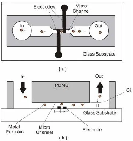
Figure 1.11: (a) Representative schematic of concept of TFC. The passage of a particle over the sensor produces a local change in temperature, which is registered by the sensor. The change can be viewed on a temperature-time plot at an arbitrarily selected point in the region just above the sensor.
Figure 1.11: (b) TFC setup with only liquid flowing through the microchannel. At any instant in time after the channel has been wetted, there is a fixed volume of liquid in contact with the heater.
Chapter 2
Computational Model
This chapter presents a computational approach to simulate the concept of TFC as described in section 1.4. The system sketch, assumptions and governing equations are described in section 2.1 while sections 2.2, 2.3 and 2.4 discuss the implementation of the model using COMSOL Multiphysics software.
2.1 Theory
TFC was by combining three domains in physics - laminar fluid flow, heat transfer and particle dynamics. Fig 2.1 shows the 2D representation of the system. The following assumptions/simplifications were made:
A 2D model was deemed sufficient to understand the concept of TFC. This is because the relevant physics can be described in a 2D model, while reducing high computational time and cost associated with a 3D model.
No material properties were assigned to the particle, since the motion of the particle could be adequately simulated using a hollow circle. In addition, since the particle boundary was thermally insulating, no thermal properti
specified for the particle.
The effect of gravity on the particle was neglected.
In accordance with the above description system were as follows:
2D continuity equation for an incomp
Figure 2.1: Geometry chosen for the computational model. The channel length and height were 8 mm and 250 µm respectively. The detection region (gray) was 180 µm long, between x=3 mm and x=3.18 mm. The particle
bottom represents the heat flux applied as a rectangle function, which is described in section 2.2.
No material properties were assigned to the particle, since the motion of the particle could be adequately simulated using a hollow circle. In addition, since the particle boundary was thermally insulating, no thermal properties were required to be specified for the particle.
The effect of gravity on the particle was neglected.
In accordance with the above description and assumptions, the governing equations for the
for an incompressible fluid:
Geometry chosen for the computational model. The channel length and height 0 µm respectively. The detection region (gray) was 180 µm long, between x=3 mm and x=3.18 mm. The particle (white) diameter was 90 µm. The red line at the bottom represents the heat flux applied as a rectangle function, which is described in section No material properties were assigned to the particle, since the motion of the particle could be adequately simulated using a hollow circle. In addition, since the particle es were required to be
, the governing equations for the
(1)
2D Navier-Stokes equation for laminar flow
subject to
Stokes equation for laminar flow with constant fluid properties:
(2)
(3) (4) (5) (6) (7) (8) (9)
2D energy equation where temperature
where a= 8 mm, b =0.3 mm, T
temperature T = T (x,y)
subject to
where a= 8 mm, b =0.3 mm, T0 = 293.15 K
(11)
(12)
(13)
(14)
(15)
The force acting on the particle is given by Newton's second law
where is the mass and
were calculated by integrating the fluid stresses over the
The boundary of the particle was treated as a moving wall whose x and y components of velocity were determined by
subject to the initial conditions
The force acting on the particle is given by Newton's second law –
is the velocity of the particle. forces acting on the particle re calculated by integrating the fluid stresses over the boundary of the particle
The boundary of the particle was treated as a moving wall whose x and y components of by eqs.(19) & (20).
subject to the initial conditions up (0) = 0 and vp (0) = 0.
(17)
forces acting on the particle of the particle.
(18)
The boundary of the particle was treated as a moving wall whose x and y components of
(19)
2.2 Numerical Model
COMSOL Multiphysics software was used to solve the governing equa section 2.1. The model was setup using four modules
DAEs, Moving Mesh, and Heat transfer in fluids.
for the flow field. The Global ODEs and DAEs module was used to solve for particle mo based on Newton's second law. The
represent the displacement of the particle. The Heat tran
temperature profile based on the flow field. All the above physics modules were solved simultaneously and were fully coupled.
velocities of the fluid. In accordance with
velocities of 1.33, 2 and 2.66 mm/s, corresponding to volumetric flow rates of 6, 9 and 12 µl/min respectively were used. The
velocities using the relation
where Q is the flow rate in m area of the channel in m2.
COMSOL Multiphysics software was used to solve the governing equations described in section 2.1. The model was setup using four modules - Laminar fluid flow, Global ODEs & esh, and Heat transfer in fluids. The laminar flow module was used to solve for the flow field. The Global ODEs and DAEs module was used to solve for particle mo based on Newton's second law. The Moving Mesh module made use of mesh movements to represent the displacement of the particle. The Heat transfer in fluids module solved for the temperature profile based on the flow field. All the above physics modules were solved simultaneously and were fully coupled. Results were obtained for three different inlet velocities of the fluid. In accordance with the parameters from the experiments, average inlet ities of 1.33, 2 and 2.66 mm/s, corresponding to volumetric flow rates of 6, 9 and 12 were used. The volumetric flow rates were converted to average
where Q is the flow rate in m3/s, is the average velocity in m/s and A is the cross
tions described in Laminar fluid flow, Global ODEs & module was used to solve for the flow field. The Global ODEs and DAEs module was used to solve for particle motion esh module made use of mesh movements to sfer in fluids module solved for the temperature profile based on the flow field. All the above physics modules were solved Results were obtained for three different inlet the parameters from the experiments, average inlet ities of 1.33, 2 and 2.66 mm/s, corresponding to volumetric flow rates of 6, 9 and 12 flow rates were converted to average
(21)
The fluid used was water. For water,
hydraulic diameter for the rectangular duct and Reynolds number for the flow were calculated using eq. (22) and (23) respectively.
where 'p' and 'q' are the sides of the rectangular cross
300 µm and q = 250 µm. The Reynolds numbers for the inlet velocities of 1.33, 2 and 2.66 mm/s, were found to be 0.448, 0.674 and 0.896 respectively
condition was specified for the fluid at the inlet of the channel. stationary for 5s while the heat flux was applied
1s. The velocity was then ramped up in time to the specified value
'pressure, no viscous stresses' condition was specified, which is physically equivalent to the fluid being released into a large stationary reservoir
as a moving wall, the x and y velocity comp
of the Global ODEs and DAEs module. The same velocity components were specified in the moving mesh module to describe the mesh displacements.
For water, = 1000 kg/m3, µ
=
8.9 x 10⁻⁴ Pa-s at 25°Chydraulic diameter for the rectangular duct and Reynolds number for the flow were calculated using eq. (22) and (23) respectively.
are the sides of the rectangular cross-sectional area of the channel. Here The Reynolds numbers for the inlet velocities of 1.33, 2 and 2.66
448, 0.674 and 0.896 respectively. An average velocity boundar condition was specified for the fluid at the inlet of the channel. The fluid was initially held stationary for 5s while the heat flux was applied and ramped up to the specified value over . The velocity was then ramped up in time to the specified value. At the outlet, the 'pressure, no viscous stresses' condition was specified, which is physically equivalent to the to a large stationary reservoir. The boundary of the particle was treated as a moving wall, the x and y velocity components of which, were determined by the output of the Global ODEs and DAEs module. The same velocity components were specified in the moving mesh module to describe the mesh displacements.
s at 25°C and the hydraulic diameter for the rectangular duct and Reynolds number for the flow were
(22)
(23)
The motion of the particle produced large deformation of the mesh, leading to potential problems with convergence. Hence, as shown in Fig 2.2, Bezier curves were used to 'assist' the moving mesh. These curves essentially prevent the formation of inverted mesh elements which may cause the solution to diverge. The speed of movement of the vertical lines was set equal to that of the particle. The horizontal lines were parametrically setup such that the line on the right of the particle reduced in length as the particle moved from left to right, while the line on the left increased in length. The solver was set to automatically remesh the domain when the specified condition of minimum mesh element quality was satisfied. Minimum element quality is essentially a measure of the symmetry of the mesh element, which goes from 0 to 1, with 1 with a perfectly symmetrical element and 0 being a degenerated element.
Figure 2.2: Bezier curves used to supplement the moving mesh. A in-built curve parameter 's' in COMSOL allows parametric conditions to be specified for the curves, which provide additional constraints that prevent inverted mesh elements.
The heater was modeled by means of a rectangle function (Fig 2.4) whose value was 1 in the region defined by the heater in the channel and was 0 everywhere else. The heat flux value was multiplied by this rectangle function so that the heat flux was non-zero only in the region of the heater. The heat flux was applied from t = 0 and allowed to ramp up to the maximum value over a time of 1s. A temperature boundary condition was set at the inlet, for the heat transfer module, and an outflow boundary condition was specified at the outlet, which assumes that convection dominates over diffusion across the outflow boundary.
The following parameters were used for the simulation and were selected to match the experimental parameters:
(a) mean radius of particle rp= 90 µm
(b) average inlet velocities of fluid = 1.33, 2 and 2.66 mm/s (c) length of the channel = 8 mm
(e) Heat flux: The heat flux used in the computational model had to be approximated from the experimental setup. In the experiments, a current of 1 mA was passed through the RTD by the multimeter, which generated heat that was then dissipated upward into the microchannel as well as downward into the silicon nitride membrane and silicon substrate. To determine the magnitude of the heat flux in both directions, a 3D model was setup in COMSOL as shown in Fig 2.3. A steady analysis was performed by considering a test section from the experimental setup. The test section included the silicon nitride membrane, the RTD and the volume of water above the membrane. Based on
of 1 µm above and below the sensor were ~ respectively.
(f) The RTD was treated as a heat source and a volumetric heat flux was supplied in W/m3. The volumetric heat
where P is the power dissipated by the RTD and is given by
‘i’ is the current of 1 mA through the RTD and ‘R’ is the resistance of the RTD ~ 670 Ω
: The heat flux used in the computational model had to be approximated from the experimental setup. In the experiments, a current of 1 mA was passed through the RTD by the multimeter, which generated heat that was then dissipated upward into the microchannel as well as downward into the silicon nitride membrane and silicon substrate. To determine the magnitude of the heat flux in both directions, a model was setup in COMSOL as shown in Fig 2.3. A steady analysis was performed by considering a test section from the experimental setup. The test section included the silicon nitride membrane, the RTD and the volume of water above the Based on the heat flux supplied the magnitudes of the heat flux at heights of 1 µm above and below the sensor were ~ 800 W/m2 and 1.6 x 10
The RTD was treated as a heat source and a volumetric heat flux was supplied in . The volumetric heat flux was calculated using the relation
where P is the power dissipated by the RTD and is given by
‘i’ is the current of 1 mA through the RTD and ‘R’ is the resistance of the
: The heat flux used in the computational model had to be approximated from the experimental setup. In the experiments, a current of 1 mA was passed through the RTD by the multimeter, which generated heat that was then dissipated upward into the microchannel as well as downward into the silicon nitride membrane and silicon substrate. To determine the magnitude of the heat flux in both directions, a model was setup in COMSOL as shown in Fig 2.3. A steady analysis was performed by considering a test section from the experimental setup. The test section included the silicon nitride membrane, the RTD and the volume of water above the the heat flux supplied the magnitudes of the heat flux at heights and 1.6 x 10⁵ W/m2
The RTD was treated as a heat source and a volumetric heat flux was supplied in
(24)
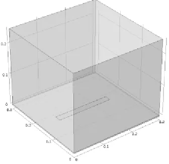
Figure 2.3: The 3D setup in COMSOL to determine the value of heat flux from the experiments. The square silicon nitride membrane of 300 µm side was at the bottom, the RTD above the membrane was 180 µm long, 20 µm wide and 200 nm high. The large block above the RTD is the volume of water that is in contact with the membrane at any given time.
2.3 Computational Results
The velocity and temperature profiles were obtained for each of the inlet velocities s section 2.2. Figs 2.5 and 2.6 show
µm particle with fluid entering the inlet at an average velocity of
obtain a signal as the particle moves over the heater region, a point was probed 50 µm above the heater and the temperature was plotted against time at this point for each particle size and at each chosen inlet velocity.
arbitrarily selected time from the solution.
Figure 2.5: Velocity profile for 90 µm particle with average fluid inlet velocity at 2 mm/s. velocity and temperature profiles were obtained for each of the inlet velocities s
and 2.6 show representative velocity and temperature profiles for a with fluid entering the inlet at an average velocity of 9 µl/min or 2
obtain a signal as the particle moves over the heater region, a point was probed 50 µm above the heater and the temperature was plotted against time at this point for each particle size and
ocity. Fig. 2.7 displays a magnified image of the moving mesh at arbitrarily selected time from the solution.
Velocity profile for 90 µm particle with average fluid inlet velocity at 2 mm/s. velocity and temperature profiles were obtained for each of the inlet velocities stated in
representative velocity and temperature profiles for a 90 /min or 2 mm/s. To obtain a signal as the particle moves over the heater region, a point was probed 50 µm above the heater and the temperature was plotted against time at this point for each particle size and magnified image of the moving mesh at an
Figure 2.6: Temperature profile for mm/s.
Figure 2.7: Magnified image showing mesh element deformation
7.4s. The axis on the right indicates the extent of deformation, with 0 representing a completely degenerate element and 1, a per
Temperature profile for 90 µm particle with average fluid inlet velocity at 2
Magnified image showing mesh element deformation around the particle The axis on the right indicates the extent of deformation, with 0 representing a completely degenerate element and 1, a perfectly symmetrical element.
fluid inlet velocity at 2
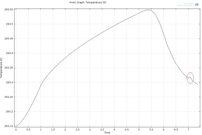
The signals obtained for a 90 µm particle at fluid velocities of 1.33, 2 and 2.66 mm/s are shown in Figs. 2.8, 2.9 and 2.10 respectively. Since the fluid was held stationary for 5s while the heat flux was ramped up, the temperature rises initially and then begins to drop once the fluid starts to flow. The particle velocity increases with increase in velocity of the fluid, the time of residency of the particle over the heater/sensor reduces. Hence, the temperature peaks become narrower with increase in velocity of the particle or in other words, the fluctuation of temperature occurs over a shorter time interval.
Figure 2.9: Predicted temperature profile for a 90 µm particle with fluid at 2 mm/s.
Figure 2.11: Comparison of the predicted signal at
Table 1 compares computationally and the analysis following it,
computational sections of this thesis could each be self
Table 1: Comparison of experimental and computational different flow rates and for a simulated heat flux value of 793 W/m
Flow Rate (µl/min) 12 9 6
Comparison of the predicted signal at 1.33, 2 and 2.66 mm/s.
compares computationally and experimentally obtained results. The same
are repeated in Chapter 4 so that the experimental and computational sections of this thesis could each be self-contained.
experimental and computational results obtained for a simulated heat flux value of 793 W/m2.
Computational Results (K) Experimental Results (K) Flow Rate (µl/min)
12 0.0018 0.0024 0.0005 0.0027 0.0046 0.0008 0.0064 0.0031 0.0015
The same table and so that the experimental and
Differences were observed in the magnitudes of experimental and computational signals at the same flow rate. The experimental and computational results differed by a factor less than 2 at flow rates of 9 and 12 µl/min. However, the factor was slightly over 2 at 6 µl/min. The amplitude of both the experimental as well as the computational result increased as the flow rate was decreased from 12 µl/min to 9 µl/min. When the flow rate was further decreased to 6 µl/min, the experimental signal dropped while a discrepancy was observed once again in the computational signal which correspondingly increased. The above discrepancy can be attributed to the mesh size and time step chosen in the model as well as the fact that the experimental signals were averaged over multiple peaks while the model contained a single particle and hence had only one peak. Ideally, an optimum mesh size must be determined in the model, for each flow rate, since the deformation of the mesh is different when the particle moves at different velocities. In this case, the mesh sizes were arbitrarily chosen and the minimum mesh size was limited by the software.
variations in the averages obtained in the two cases.
In general, the differences in experimental and computational signal can be attributed to the assumptions made in the computational model as well as experimental constraints. The model was 2D in nature and this resulted in an error while extrapolating the physics of particle motion and its response to heat, from the model to the experiment. In the experiments, the particle was 90 µm wide and it occupied less than a third of the channel width. In the simulation, the 2D model is assumed to have a default depth of 1m, which meant that the particle occupied the entire width of the channel as well as the sensor. The particle in the experiment was spherical in shape. The 2D particle in the model is cylindrical when extrapolated to 3D.The particle in the numerical simulation was considered to be perfectly insulated. The polystyrene beads used in the experiment had a low but non-zero value of thermal conductivity. The particle in the model maintained a constant height as it moved through the microchannel. In the experiments, the particles were suspended using glycerol and they were drawn into the channel from a reservoir which did not ensure constant height of the particles.
At a low flow rate of 6 µl/min, the time of residency of the particle over the sensor is maximum, which allows for a temperature gradient to develop in the detection region and the signal at the lowest flow rate is therefore higher than that at the highest flow rate.
In summary, it was found that the experimental and computational results at 9 and 12 µl/min were in reasonable agreement, given the assumptions made while the results at 6 µl/min were close in value but differed in relative trend.
2.4 Numerical accuracy of computational model
Chapter 3
Materials and Methods
This chapter discusses the design and construction of the device used for TFC. Over the duration of this research, multiple generations of devices were developed and tested before one was found to be best suited for the application.
3.1 General Device Schematic
3.2 Experimental Setup
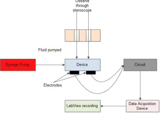
Fig. 3.2 describes the experimental setup for TFC. Once the device was fabricated and tubes were inserted into the two ports, one of the tubes was connected to a syringe fixed onto a syringe pump. This formed the inlet tube. The suspension containing the polystyrene beads was pumped through the microchannel through this tube. The other tube was the outlet tube and it was immersed in a container filled with water, to create a stable outlet condition. For the approach using the inlet tube, this outlet condition was critical since the output signal was very sensitive to the exit condition of the fluid. As explained in the sections ahead, the inlet tube was eliminated in the later generations of devices.
The PDMS block was bonded such that the RTD was one the lower side of the glass substrate. The RTD heated the glass and this heat was then transferred to the fluid by conduction and convection. Fig. 3.3 shows the design of the heater coil used for the first, second and third generation devices. One metallic pin each was attached by means of a fixture to the square pads (not seen in figure) at the ends of the nickel coil. These formed the electrodes across which the output signal was measured. The electrodes were connected to an analog circuit designed on a breadboard. The circuit was designed to take a reference voltage as input and provide a constant current as output. This constant current was fed to the device through the same pair of electrodes mentioned above.
The flow of current through the coil generates heat which is dissipated into the channel. The device was connected to a breadboard circuit and a data acquisition device (DAQ). The signal from the device was recorded using the DAQ which was interfaced with LabView to write the data to an output file. The flow of fluid in the microchannel was observed under a stereoscope. Fig 3.4 shows the fixture that was used to clamp the device and Fig 3.5 shows the device held in the fixture under the stereoscope. The device shown in the figure is a third generation device with the substrate flipped so that the RTD was inside the microchannel.
Figure 3.5: Device held in fixture under a stereoscope and connected to a syringe pump (not seen in figure) with electrode pins connected.
3.3 Microfabrication
This section discusses the general procedure to fabricate the device described in the previous section. This consisted of the following steps -
3.3.1 Fabrication of substrate
3.3.1 Fabrication of Substrate For the first, second and third
of depositing nickel, which formed the RTD.
Kunduru, a Ph.D candidate in Dr. Glenn Walker's lab.
acetone and IPA, followed by a baking process for dehydration, which 20 minutes. A small amount of photoresist AZ 5214
a quarter dollar coin. The substrate
seconds, which formed a 1.4 µm thick photoresist layer.
110◦C for about a minute. After soft baking, the photoresist layer
light for 8 seconds. To develop the pattern formed, the substrate photoresist developer MIF-CD 26 for 60 seconds and then rinsed with
using a nitrogen spray. Fig 3.6 outlines the process flow for the above fabrication.
Figure 3.6: Process flow diagram for fabrication of negative photoresist. Nickel was deposited to a height of
ubstrate
and third generation devices, a glass substrate was used for the purpose , which formed the RTD. The substrates were fabricated by Vindhya candidate in Dr. Glenn Walker's lab. The glass substrate wa
, followed by a baking process for dehydration, which was done at 200 es. A small amount of photoresist AZ 5214 was added to the substrate, to the size of a quarter dollar coin. The substrate was then subjected to spin coating at 4000 rpm for 45 seconds, which formed a 1.4 µm thick photoresist layer. This was followed by sof
C for about a minute. After soft baking, the photoresist layer was exposed
light for 8 seconds. To develop the pattern formed, the substrate was immersed in the CD 26 for 60 seconds and then rinsed with DI
Fig 3.6 outlines the process flow for the above fabrication.
Process flow diagram for fabrication of glass substrates. AZ 5214 was used as a photoresist. Nickel was deposited to a height of ~ 200 nm using e-beam deposition.
s used for the purpose The substrates were fabricated by Vindhya was cleaned using s done at 200◦C for s added to the substrate, to the size of s then subjected to spin coating at 4000 rpm for 45 s followed by soft baking at s exposed under UV
s immersed in the DI water and dried Fig 3.6 outlines the process flow for the above fabrication.
As shown in Fig 3.3, there were two coils on the substrate. To create the second coil, the image was reversed. The substrate was baked at 115◦C for 20 minutes. It was then coated
with the photoresist and spun at 4000 rpm for 45 seconds, which gave a photoresist layer of about 1.4 µm. The substrate was then soft-baked at 90◦C for 2 minutes and later exposed to
UV light for 2 seconds. Once the exposure was complete, the substrate was baked again on a hotplate at 116◦C for 3 minutes. It was then subjected to flood exposure (without a filter) for
45 seconds. Development of the exposed substrate was done using the developer MIF-CD 26 for 30 seconds with slight agitation. After developing, the substrate was rinsed with DI water and dried with a nitrogen gun.
An electron beam evaporator was used to deposit a 200 nm thick film of nickel (Kurt Lesker, 99.99% pure) on the patterned glass substrates. The nickel-coated substrates were then treated with acetone to lift off nickel from the un-patterned areas, rinsed with DI water, and dried with nitrogen. The sensor was designed to have a nominal resistance of 270 ohms at room temperature.
The nickel pattern was created using e-beam deposition and such that the sensor, in the form of a single meander, was at the center of the membrane (shown later in Fig 3.18).
3.3.2 Fabrication of SU8 master for PDMS Channels
The first step in making PDMS channels was to fabricate a master out of the high-aspect ratio photoresist SU-8. An overview of the process is shown in Fig 3.7. Masks for photolithography were designed using Adobe Illustrator. For the application of TFC, a straight channel with a rectangular cross-section, was deemed to be sufficient. The background of the mask was black in color while the channel was white. When the mask is printed on a transparency, the channel turns out to be transparent while its surroundings are opaque. This is crucial for the process of photolithography when using a negative photoresist.
Figure 3.8: Graph of photoresist film thickness obtained vs spin speed. Source: MicroChem
For positive photoresists, the reverse is true, i.e, the exposed part of the photoresist is eliminated at the time of developing while the unexposed part is retained.
Table 2: Soft Baking - time and temperature settings for a range of photoresist thickness. Source: MicroChem.
Thickness (µm) Soft Bake Time (mins) 65°C
Soft Bake Time (mins)
95°C
25-40 0-3 5-6
45-80 0-3 6-9
85-110 5 10-20
115-150 5 20-30
160-225 7 30-45
Table 3: Exposure time and intensity settings for a range of photoresist thickness. Source: MicroChem.
Thickness (µm) Energy Exposure (mJ/cm2)
25-40 150-160
45-80 150-215
85-110 215-240
115-150 240-260
Table 4: Post-Exposure Baking Time and temperature settings for a range of photoresist thickness. Source: MicroChem.
Thickness (µm) PEB Time (mins) 65°C
PEB Time (mins) 95 °C
25-40 1 5-6
45-80 1-2 6-7
85-110 2-5 8-10
115-150 5 10-12
160-225 5 12-15
3.3.3 PDMS Molding
To create the PDMS mold, about 30g of PDMS pre-polymer (PDMS base) was poured into a weigh boat and mixed with 3g of cross-linker. The amount of base used depends on the final thickness of the polymer device desired. A thin layer facilitates bonding with the glass substrate. The mixture was stirred continuously with a plastic fork for about 5 minutes. The weight boat was then placed in a desiccator and subjected to a vacuum until all the air bubbles in the mixture disappeared.
The petri dish was then placed on a hotplate and the temperature was ramped up to 115◦C and maintained for about 5 minutes. Once the PDMS had cured completely, the wafer, combined with the PDMS layer was separated from the petri dish using a spatula and the PDMS layer was peeled off the wafer. Sections of the PDMS with the channel designs on them were cut out and bonded to chips to form devices. Fig 3.9 shows a representative block of PDMS containing straight channels.
Figure 3.9: Representative channels fabricated in a PDMS mold. Blocks were cut out, each containing one channel, and bonded to a substrate. Red arrows point to the channels formed in the block.
3.4 First Generation Devices
No significant data was obtained for solid beads through the use of these devices. However, encouraging data was collected through the use of the T-junction channel shown in Fig 3.11. This T-junction device was used to produce water-slugs by passing DI water through one inlet and air through the other. The results are shown in Chapter 4. The circuit used for these devices is described in section 3.4.1.
(a)
(b)
Figure 3.11: Mask with T-junction channel included for testing the device using water-slugs. The channels in the first and second row are 1 mm wide. The channels in the third row are 0.3 mm wide. The remaining channels were not used.
Figure 3.12: The completed first generation device. PDMS block thickness and tube length were optimized in later designs.
3.4.1 Circuit for First Generation Devices
Figure 3.13: Constant current circuit used t 2009).
Figure 3.14: Block diagram of
on a breadboard and connected to a data acquisition system (NI USB
Constant current circuit used to power the fabricated device. Source:
Block diagram of the first generation of the analog circuit that was constructed on a breadboard and connected to a data acquisition system (NI USB-6009).
Source: (Zhao et.al
The device resistance forms RLOAD shown in Fig 3.14. The circuit was operated with inputs of +15 V and -15V supplied from an Agilent E3649A power source. The heating electrodes of the device were connected across the heating or excitation circuit and a reference voltage of 0.6 V was provided to the circuit. This produced a constant current of about 6 mA through the coils. As per the working theory described in section 3.2, differential heating of fluid and solids was anticipated, which would produce a change in temperature in the region above the heater in the channel and this would be sensed by the electrodes. The fluctuation was expected to be too small to notice without aid and hence the signal was amplified via the sensing circuit before it was recorded. The sensing circuit consisted of three instrumentation amplifiers and a differential amplifier. The output signal was fed to the first instrumentation amplifier and offset by a DC voltage supplied to a second amplifier. This DC voltage was equal in sign and magnitude to the signal. The function of the differential amplifier was to multiply the difference of the signal and the offset by its gain. The result from this amplifier was fed to the third instrumentation amplifier which further multiplied the result by its gain. The output of the third instrumentation amplifier was fed to both the oscilloscope as well as a data acquisition device (DAQ- NI USB-6009).The device was interfaced with the software LabView to monitor and record signals from the device.
This could be gauged by a sharp drop in voltage on an Oscilloscope connected to the circuit.
3.5 Second Generation Devices
To overcome the problem of tube clogging in the first generation of devices, an alternative was proposed and successfully tested. In these second generation devices, the inlet tube was eliminated and the inlet port was widened. Once it was bonded, the widened port served as a reservoir or well for the suspension containing beads, as shown in Fig 3.9. The syringe pump was then connected to the outlet tube and instead of pumping, the suspension was withdrawn through the channel. This was found to greatly enhance the number of beads passing through the channel. However, the beads still tended to settle quickly in the reservoir. To counter this problem, the beads were balanced using glycerol, as described in section 3.8. By balancing the densities of the beads and the fluid, the beads could be suspended indefinitely. Narrower channels of 0.3 mm width were used in the second generation of devices.
Despite observing several beads passing through the channel during a specific time interval, no signal was obtained with these devices.
lack of data. The glass substrate was too thick to register a change i passage of a 90 µm bead above it. This
signal from the device or in other words, the sensitivity of the problems were eliminated in the third generation of devices.
generation of devices is described
3.5.1 Circuit for Second Generation
Figure 3.16: Block diagram of
additional instrumentation amplifiers from the first generation circuit were eliminated to prevent saturation of the circuit.
Despite observing several beads passing through the channel during a specific time interval, no signal was obtained with these devices. The substrate was determined as the cause
he glass substrate was too thick to register a change in temperature due to the µm bead above it. This relatively large thickness was likely to make any
or in other words, the sensitivity of the device
problems were eliminated in the third generation of devices. The circuit used for the second generation of devices is described in the following section.
eneration Devices
Block diagram of the second generation of constant current circuits
instrumentation amplifiers from the first generation circuit were eliminated to prevent saturation of the circuit.
Despite observing several beads passing through the channel during a specific time interval, as the cause for the n temperature due to the relatively large thickness was likely to make any was low. These The circuit used for the second
To overcome the problem of saturation in the first generation circuit, the instrumentation amplifiers were eliminated in the second generation circuits. The signal from the device and the DC offset were both fed to the first differential amplifier which multiplied their difference by its gain and fed the result to an instrumentation amplifier. The amplified output from the op-amp was fed to the oscilloscope and the DAQ.
3.6 Third Generation Devices
Figure 3.17: Third generation of devices which differed from the second generation only in the orientation of the substrate. The substrate was flipped over so that the RTD was inside the channel.
3.6.1 Circuit for Third Generation Devices
The circuit used for the third generation of devices was the same as that used for the previous generation.
3.7 Fourth Generation Devices
Figure 3.18: (top left) Silicon substrate patterned with nickel and (top right) magnified image of the sensor on the substrate. (bottom right) Diagram of enlarged sensor pattern. The width of the nickel strip was approximately 10 µm. (bottom left) 2D schematic of substrate.
3.8 Preparation of Sample Suspension and Flow Conditions
The balancing agent used was glycerol and quantities of the different substances were added according to the formula -
1 1 2 2
1 2
V d V d D
V V
(26)
where D is the density of the final suspension, which must equal the density of the beads for them to be suspended. V1 ,d1, V2 and d2 are the volumes and densities of the carrier fluid and balancing agent respectively. For any arbitrarily chosen volume of the carrier fluid, the above formula gives the volume of the balancing medium required, when the density of the solid particles is known.
For the first generation devices, separate suspensions were prepared using bead sizes of 25 µm and 90 µm. The 25 µm particles were too small to elicit any response from the sensor. Hence, with the size of the heater coils in mind, the 90 µm bead suspension was chosen for subsequent experiments.
Chapter 4
Results and Discussion
Repeatable experimental results were obtained with the final generation devices. Results were obtained for three arbitrarily chosen flow rates of 6, 9 and 12 µl/min. Data was recorded for 30 seconds in case of solid particles. Test results with the first generation of results are also presented in the following section.
4.1 Results with First, Second and Third Generation Devices
Figure 4.1: MATLAB plot of voltage amplitude against time. The sharp peaks indicate the response to a disturbance introduced into the circuit by blowing air over it.
Figure 4.2: (left) Shift in baseline voltage (y-axis) due to change in flow rates. (right) Schematic of device used for the measurement. Fluid was pumped in through the inlet tube at different flow rates and the corresponding signal was recorded.
4.2 Results with Water-Slugs
Figure 4.3: Detection of DI water-slugs in the microchannel. The size of the slugs relative to the channel and the sensor, ensured distinct signals.
4.3 Results with Fourth Generation Devices
(a)
(b)
(c)
4.4 Discussion
With the first generation of devices no significant data was obtained with solid particles due to the clogging of the particles in the inlet tube and at the bottom of the inlet port. In addition, the analog circuit designed was found to saturate often, thus preventing any data collection.
For the second generation of devices, the width of the channel was reduced and smaller sensors were used. Other problems with the first generation of devices, such as difficulty in passage of beads, was reduced by creating a reservoir in the PDMS block and withdrawing the beads through the channel instead of pumping them through it. However, these devices did not produce any noteworthy results. This was because the presence of the glass substrate between the RTD and the channel reduced the heat dissipated into the channel.
In the final generation of devices, a multimeter was used to measure resistance changes in the RTD due to a changes in its temperature. The multimeter was considerably more sensitive than the analog circuit constructed and along with the approach in the third generation of devices, was instrumental in achieving the expected results. The multimeter had precision up to 6 decimal places, which made it suitable for the detection of 90 µm particles, which produced signals on the order of 0.001 K.
The size of the bead relative to that of the sensor was an important parameter in the use of this device. In the case of 90µm beads, the distance between the sensor (located in the center of the channel) and the channel wall, was larger than the diameter of the beads. It was found that beads passing the sensor along the edge of the channel were sometimes undetected or the signal was vague. As seen in Fig 4.4, the experimental results with solid particles were obtained in the form of change in resistance. This change was converted to a temperature difference using the relation
R = R 1f 0
α T
(27)
or
R / R0 α T
(28)
The raw data was analyzed and the points corresponding to the peak values were located. Twenty data points on either side of the peak value were summed up and averaged to calculate
R
,
which formed the mean value or baseline.R
was the peak value. Using thesevalues,
∆
T
was calculated for each peak. The arithmetic mean and standard deviation of the different values of∆
T
were calculated to determine the average amplitude of temperature change at each flow rate. Raw data for computational results were analyzed in a similar manner to determine the average amplitude of the signal. The averaged experimental and computational results are as tabulated in Table 5. Standard deviations for the averaged experimental peak amplitudes were found to be 15 x 10-4 at 6 µl/min, 8.79 x 10⁻⁴ at 9 µl/min and 5 x 10⁻⁴ at 12 µl/min. The numbers of particles detected at 6 µl/min and 9 µl/min were small, leading to larger standard deviations.The output of the function is the mean and standard deviation of the data with respect to the vertical axis of symmetry. The FWHM was then calculated using the relation
where σ is the standard deviation.
The FWHM at 6, 9 and 12 µl/min were
The standard deviations for the different peaks at each flow rate were arithmetically averaged to find the FWHM. The averaged FWHM
indicating a reduction in time of residency of the particle over the heater/sensor.
Figure 4.5: Representative illustration of full width at half maximum (FWHM) for a signal peak.
ion is the mean and standard deviation of the data with respect to the vertical axis of symmetry. The FWHM was then calculated using the relation
FWHM = 2.35482 * σ is the standard deviation.
The FWHM at 6, 9 and 12 µl/min were 3.11 x 10⁻³, 2.98 x 10⁻³ and 1.96 x 10
The standard deviations for the different peaks at each flow rate were arithmetically averaged he FWHM. The averaged FWHMs were found to decrease with increase in flow rate indicating a reduction in time of residency of the particle over the heater/sensor.
Representative illustration of full width at half maximum (FWHM) for a signal ion is the mean and standard deviation of the data with respect to the vertical axis of symmetry. The FWHM was then calculated using the relation
(29)
1.96 x 10⁻³ respectively. The standard deviations for the different peaks at each flow rate were arithmetically averaged decrease with increase in flow rate, indicating a reduction in time of residency of the particle over the heater/sensor.
Table 5: Comparison of experimental and computational results at a simulated heat flux value of 793 W/m2.
Computational Results (K) Experimental Results (K) Flow Rate (µl/min)
12 0.0018 0.0024∓ 0.0005 9 0.0027 0.0046∓ 0.0008 6 0.0064 0.0031∓ 0.0015
Table 5 compares the temperature difference (∆T) obtained from the experiments with the