New Functional Data Methods for Neuroimaging Data.

ABSTRACT

MA, WANYING. New Functional Data Methods for Neuroimaging Data. (Under the direction of Luo Xiao.)

Because of technology advancement in both the processing and storage of large data sets,

functional data has become common in many scientific areas nowadays. Neuroimaging techniques

which allows for the further understanding of the brain inner working with disease diagnosis,

cognitive process and psychological process have seen a explosive growth of cross-disciplinary

research work in this field. The complex structures of neuroimaging data have posed special

challenges and opportunities for functional data analysis. In this thesis, we are motivated by

neuroimaging studies and propose new methods for functional data analysis.

In Chapter 2, motivated by a functional magnetic resonance imaging (MRI) study on pain

caused by thermal stimuli applied to human subjects, we propose a new functional mixed model

for scalar on function regression. The model extends the standard scalar on function regression for

repeated outcomes by incorporating subject-specific random functional effects. Using functional

principal component analysis, the new model can be reformulated as a mixed effects model and

thus easily fit. A test is also proposed to assess the existence of the subject-specific random

functional effects. We evaluate the performance of the model and test via a simulation study, as

well as on data from the motivating fMRI study of thermal pain. The data application indicates

significant subject-specific effects of the human brain hemodynamics related to pain and provides

insights on how the effects might differ across subjects.

In Chapter 3, motivated by a diffusion tensor imaging (DTI) study of sports-related concussion

(SRC) on college football athletes, we propose a combination of functional data methods and

feature selection methods to differentiate two classes of athletes, players with concussion and

players without concussion. To deal with the inherent difficulty of aligning the brain tracts

across human subjects, we propose to consider the densities of scalar observations along the

tracts. Then we transform the densities to functional data, for which we apply functional

principal component analysis to extract features. As there is a large number of features, we

propose to use a K-means based probabilistic subset search (PSS) method to conduct feature

clustering, which is essential due to the heterogeneous nature of SRC. The proposed methods

are applied to the motivating DTI study and identify a small subset of features that provides

good out-of-sample classification accuracy. Moreover, 2 subgroup clusters are identified for the

© Copyright 2019 by Wanying Ma

New Functional Data Methods for Neuroimaging Data

by Wanying Ma

A dissertation submitted to the Graduate Faculty of North Carolina State University

in partial fulfillment of the requirements for the Degree of

Doctor of Philosophy

Statistics

Raleigh, North Carolina

2019

APPROVED BY:

Anarb Maity Rui Song

Xinge Jeng Luo Xiao

DEDICATION

BIOGRAPHY

The author was born in November 1993 and grew up in Henan, China. Before she came to United

States, she earned her Bachelor of Science degree in Statistics from School of Mathematical

Sciences at Beijing Normal University in May of 2014. Later in August, she went to North

Carolina State University to pursue the Ph.D. degree in Statistics at Department of Statistics.

In May of 2017, she earned the Masters degree in Statistics at NC State, and she will defend

ACKNOWLEDGEMENTS

First and foremost, I would like to express my deepest and sincerest gratitude to my advisor, Dr.

Luo Xiao for his infinite support and professional guidance throughout my graduate research. For

the past three and a half years, Dr. Xiao devoted the endless patience and time to prepare me

well for the projects, help me get through the challenges, provide insightful suggestions, sharpen

my presentation skills and academic writing skills, and show me great examples for both scientific

research and co-working. His great passion to research, earnest attitude, broad knowledge in

statistics, professionalism have deeply inspired me and will always be the motivation to further

improve myself in my career development. I feel truly grateful to ever have him as my advisor.

I would also like to thank Dr. Arnarb Maity, Dr. Rui Song, Dr. Jessie Jeng and Dr. Lokendra

Pal for being my committee members and their valuable comments with regard to my dissertation.

I also feel really fortunate to be a member of the big Statistics family at North Carolina State

University, and I would like to extend my sincere appreciation to the whole Statistics graduate

program. This will be the most important experience in my life, and it is such a wonderful thing

to have you in this memory. In particular, I am very thankful to Dr. Wenbin Lu for his help

on my graduate study as the director of graduate program, and I am very grateful to both

Lanakila Alexander and Alyson McCoy for answering my countless questions. Many thanks to

my dear friends, Benjamin Hu, Dr. Cai Li, Dr. Stephanie Chen, Dr. Munir Winkle, Dr. Yuan

Feng, Ruonan Li for their supports and companion.

I would like to thank my mentors Dr. Mona Liu and Dr. Jian Zhu from Takeda, Dr. Radha

Mohanty from Bayer Crop Science, and Dr. Youlan Rao from United Therapeutics. Thank you

for providing these great internship opportunities and sharing your life experience with me. Your

training, help and advice are one of the most important assets for me to prepare for my future

career.

Last but not least, I want to thank my dear parents and brother. You give me the unconditional

love and supports, cheer me up whenever I feel down in my life, and give me the strength to

face every challenge. Without your trust, understanding and supports, I can never make it this

TABLE OF CONTENTS

LIST OF TABLES . . . vii

LIST OF FIGURES . . . .viii

Chapter 1 Introduction . . . 1

1.1 General Description . . . 1

1.2 Univariate Functional Data . . . 6

1.2.1 Functional principal component analysis . . . 6

1.2.2 Scalar on function regression . . . 8

1.3 Repeatedly Observed Functional Data . . . 9

1.4 Multivariate Functional Data . . . 11

1.5 Research Projects . . . 12

Chapter 2 A Functional Mixed Model for Scalar on Function Regression with Application to a Functional MRI Study. . . 15

2.1 Introduction . . . 15

2.2 Method . . . 18

2.2.1 Functional mixed model for scalar on function regression with repeated outcomes . . . 18

2.2.2 Model for the repeated functional predictor . . . 19

2.2.3 Model estimation . . . 20

2.2.4 Test of random functional effect . . . 22

2.3 Extension to Multivariate Functional Predictor . . . 24

2.4 A Simulation Study . . . 26

2.4.1 Simulation settings . . . 26

2.4.2 Results on tests . . . 27

2.4.3 Results on estimation . . . 29

2.5 Data Application . . . 30

2.6 Discussion . . . 33

Chapter 3 Flexible Feature Selection and Cluster Analysis for Heterogeneous Data With Application to Diffusion Tensor Imaging Study . . . 35

3.1 Introduction . . . 35

3.1.1 Data description . . . 38

3.2 Data Preprocessing and Feature Extraction . . . 39

3.2.1 Density covariates . . . 39

3.2.2 Functional principal component analysis for densities . . . 39

3.3 Cluster Analysis and Feature Selection . . . 40

3.4 Results . . . 43

3.5 Discussion . . . 48

BIBLIOGRAPHY . . . 49

APPENDICES . . . 56

Appendix A Supplemental Materials for Chapter 2 . . . 57

A.1.1 Additional simulation results for FMM with a univariate functional

predictor . . . 58

A.1.2 A simulation study for FMM with a multivariate functional predictor 58 A.1.3 Additional results for the data application . . . 66

A.1.4 Additional simulation results for the power of the tests . . . 66

A.2 Fast Covariance Estimation for Multivariate Functional Data . . . 66

A.2.1 Fundamental theory . . . 66

A.2.2 Data structure . . . 76

A.2.3 Covariance estimation . . . 77

Appendix B Supplemental Materials for Chapter 3 . . . 80

B.1 Results for Greedy Search . . . 80

LIST OF TABLES

Table 2.1 Results of FMM and FLM for separate and joint analysis of the fMRI data. 30

Table 3.1 PSS clustering results using the firstpselected features and the distribution of the true group in the estimated clustering membership. . . 47

Table A.1 Sizes of three tests at the 5% level for correlated and independent univariate functional predictorXij(t).I: number of subjects;J: number of visits per subject;r: noise level in the functional predictor. . . 59 Table A.2 Estimation/prediction errors of FMM and FLM across 1000 data sets

with a univariate functional predictor under various model conditions. . . 59 Table A.3 Estimation/prediction errors of FMM and FLM across 1000 data sets

with a univariate functional predictor under various model conditions. . . 61 Table A.4 Estimation/prediction errors of FMM and FLM across 1000 data sets

with a univariate functional predictor under various model conditions. . . 61 Table A.5 Estimation/prediction errors of FMM and FLM across 1000 data sets

with a univariate functional predictor under various model conditions. . . 62 Table A.6 Multivariate functional predictor: Sizes of three tests at the 5% level

for correlated and independent functional predictor Xij(t). I: number of subjects; J: number of visits per subject; r: noise level in the functional predictor. . . 62 Table A.7 Multivariate functional predictor: Estimation/prediction errors of FMM

and FLM across 1000 data sets under various model conditions. . . 63 Table A.8 Multivariate functional predictor: Estimation/prediction errors of FMM

and FLM across 1000 data sets under various model conditions. . . 64 Table A.9 Multivariate functional predictor: Estimation/prediction errors of FMM

and FLM across 1000 data sets under various model conditions. . . 65 Table A.10 Multivariate functional predictor: Estimation/prediction errors of FMM

LIST OF FIGURES

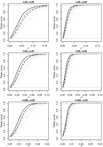
Figure 2.1 Data from the fMRI study: (a) and (c) give the fMRI time series at ROI LAIns for two subjects each with three repetitions; (b) presents the corresponding spaghetti plots of pain ratings. . . 17 Figure 2.2 Power of three tests at the 5% level for the correlated functional predictor

Xij(t) and as a function of τ2. Black lines are for smooth functional data, i.e.,r= 0 while gray lines are for noisy functional data. Solid lines: equal-variance test; dashed lines: Bonferroni-corrected test; dot-dashed lines: asLRT. . . 28 Figure 2.3 Estimated functional effect with a joint analysis of 6 ROIs using FMM.

The black solid line is the population functional effect β(t) +δ(t) when the hot stimuli is applied; the gray dashed curves are the subject-specific random functional effectβ(t) +δ(t) +βi(t). . . 32 Figure 2.4 Estimated functional effect with a separate analysis of ROI RAIns I and

ROI RThal using FMM. The thick solid line is the population functional effectβ(t) +δ(t) when the hot stimuli is applied; the black solid curves areβ(t) +δ(t) +βi(t) for one cluster of the subjects and the gray dashed curves are another cluster. . . 33

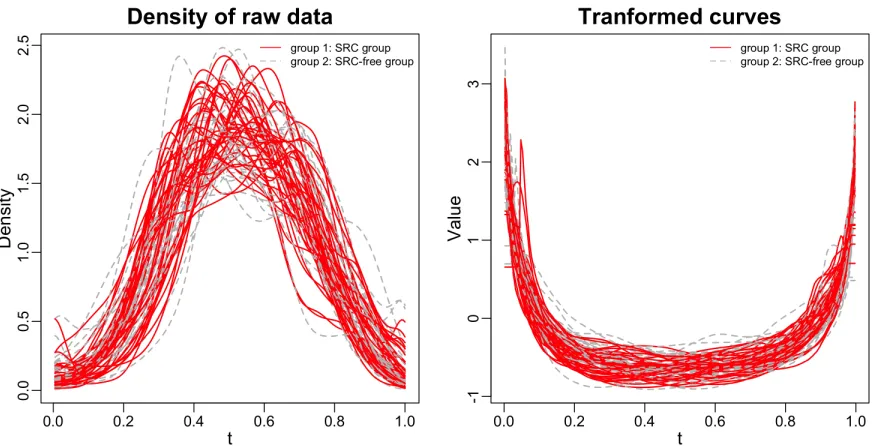
Figure 3.1 Comparison of the raw data density and the log-quantile transformed curves at tract cst r using measurement FA. The left panel shows the density of the raw data; right panel shows the log-quantile transformed curves. Note that for both the two density calculation, we scaled the data and de-outlier as discussed in Section 3.2. . . 37 Figure 3.2 PSS method using different starting values vs. greedy search:

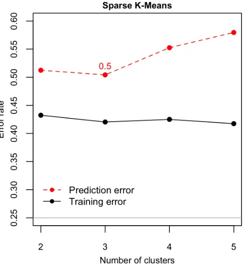
Out-of-sample classification error by 100 times bootstrapped 5-fold cross-validation at each step of selected features. Solid red lines are for greedy search. Blue dashed lines are for PSS method. Note that in each subfig-ure, greedy search use the corresponding pre-specified fixed number of clusters shown in the title to select feature at each step; while PSS uses the selected features given by greedy search as starting value at each step. 45 Figure 3.3 Sparse K-means using different number of clusters: Out-of-sample

clas-sification error by 100 times bootstrapped 5-fold cross-validation. Solid black line is for training error. Red dashed line is for prediction error. . . 45 Figure 3.4 Lasso: Out-of-sample classification error by 100 times bootstrapped 5-fold

cross-validation. Left panel displays different error types. Right panel displays the model complexity selected by Lasso. . . 46 Figure 3.5 p= 2: Plots of the in-sample estimated clustering membership vs. the

Figure A.1 Power of three tests at the 5% level for the independent univariate functional predictorXij(t) and as a function of τ2. Black lines are for smooth functional data, i.e.,r= 0 while gray lines are for noisy functional data. Solid lines: equal-variance test; dashed lines: Bonferroni-corrected test; dot-dashed lines: asLRT. . . 60 Figure A.2 Multivariate functional predictor: Power of three tests at the 5% level

for the correlated functional predictor Xij(t) and as a function of τ2. Black lines are for smooth functional data, i.e.,r= 0 while gray lines are for noisy functional data. Solid lines: equal-variance test; dashed lines: Bonferroni-corrected test; dot-dashed lines: asLRT. . . 63 Figure A.3 Multivariate functional predictor: Power of three tests at the 5% level

for the independent functional predictorXij(t) and as a function of τ2. Black lines are for smooth functional data, i.e.,r= 0 while gray lines are for noisy functional data. Solid lines: equal-variance test; dashed lines: Bonferroni-corrected test; dot-dashed lines: asLRT. . . 64 Figure A.4 Residual plot of error term using joint analysis with FMM. Red line

denotes the normal density curve fitted over the error. . . 67 Figure A.5 Residual plot of random errors using univariate analysis with FMM. Red

line denotes the normal density curve fitted over the error. . . 67 Figure A.6 Violin plots of estimation errors for both joint analysis and separate

analysis of ROIs using FMM and FLM. Note that the mean squared error is first averaged within each subject. The red dashed curve is the median of MSE given by FMM. . . 68 Figure A.7 Scenario 1: Power of three tests at the 5% level for the univariate

corre-lated functional predictorXij(t) and as a function ofτ2. Black lines are for smooth functional data, i.e.,r= 0 while gray lines are for noisy functional data. Solid lines: equal-variance test; dashed lines: Bonferroni-corrected test; dot-dashed lines: asLRT. . . 68 Figure A.8 Scenario 1: Power of three tests at the 5% level for the univariate

in-dependent functional predictor Xij(t) and as a function of τ2. Black lines are for smooth functional data, i.e., r = 0 while gray lines are for noisy functional data. Solid lines: equal-variance test; dashed lines: Bonferroni-corrected test; dot-dashed lines: asLRT. . . 69 Figure A.9 Scenario 2: Power of three tests at the 5% level for the univariate

corre-lated functional predictorXij(t) and as a function ofτ2. Black lines are for smooth functional data, i.e.,r= 0 while gray lines are for noisy functional data. Solid lines: equal-variance test; dashed lines: Bonferroni-corrected test; dot-dashed lines: asLRT. . . 70 Figure A.10 Scenario 2: Power of three tests at the 5% level for the univariate

in-dependent functional predictor Xij(t) and as a function of τ2. Black lines are for smooth functional data, i.e., r = 0 while gray lines are for noisy functional data. Solid lines: equal-variance test; dashed lines: Bonferroni-corrected test; dot-dashed lines: asLRT. . . 71 Figure A.11 Multivariate functional predictor with Scenario 1: Power of three tests

Figure A.12 Multivariate functional predictor with Scenario 1: Power of three tests at the 5% level for the independent functional predictor Xij(t) and as a function ofτ2. Black lines are for smooth functional data, i.e.,r = 0 while gray lines are for noisy functional data. Solid lines: equal-variance test; dashed lines: Bonferroni-corrected test; dot-dashed lines: asLRT. . 73 Figure A.13 Multivariate functional predictor with Scenario 2: Power of three tests

at the 5% level for the correlated functional predictor Xij(t) and as a function of τ2. Black lines are for smooth functional data, i.e., r = 0 while gray lines are for noisy functional data. Solid lines: equal-variance test; dashed lines: Bonferroni-corrected test; dot-dashed lines: asLRT. . 74 Figure A.14 Multivariate functional predictor with Scenario 2: Power of three tests

at the 5% level for the independent functional predictor Xij(t) and as a function ofτ2. Black lines are for smooth functional data, i.e.,r = 0 while gray lines are for noisy functional data. Solid lines: equal-variance test; dashed lines: Bonferroni-corrected test; dot-dashed lines: asLRT. . 75

Figure B.1 Greedy search based on transformed curves: Out-of-sample classification error by 100 bootstrapped 5-fold cross-validation at each step of selected features. Solid black lines are for training error. Red dashed lines are for prediction error. Note that in each subfigure, greedy search use the corresponding pre-specified fixed number of clusters shown in the title to select feature at each step. . . 81 Figure B.2 Greedy search based on raw data using different number of clusters:

Out-of-sample classification error by 100 bootstrapped 5-fold cross-validation at each step of selected features. Solid black lines are for training error. Red dashed lines are for prediction error. Note that in each subfigure, greedy search use the corresponding pre-specified fixed number of clusters shown in the title to select feature at each step. . . 82 Figure B.3 p= 3: Plots of the in-sample estimated clustering membership vs. the

CHAPTER

1

INTRODUCTION

1.1

General Description

Functional data analysis (FDA) has kept raising research interests in recent decades. As the

technology developments in the measurement accuracy and storage of large data sets, a variety

of machines and devices across many scientific domains have been well designed to enable

the continuous monitoring of data observations, which results in the functional or imaging

data types. For example, one can consider the functional magnetic resonance imaging (fMRI)

brain scan data set, where a continuous brain scan was made for each of 20 participants over

several visits in a fMRI pain study, producing fMRI time series that consist of 23 equidistant

temporal measurements of brain activation. These fMRI time series were recorded for each of

21 pain-responsive regions of interest over the brain for each participant at each visit. In FDA,

the fMRI time series of the brain activation measurements are viewed as a function of time.

Different from the traditional data format, functional data treats the function or curve as a

functional data. The intrinsically infinite dimensional property of functional data has naturally

posed challenges for the purposes of testing, regression and clustering in many scientific areas,

and researchers have made great contribution in solving these problems and further developing

the methods and tools in FDA; see [Ram06; Wan16] for a comprehensive overview.

Functional data is often observed in a continuous manner on a fixed or random (time

or location) grid, and typically consists of a series of curves. The core assumption in FDA

is smoothness, that is, it is assumed that the actual observed functional data is the noisy

observation of a true underlying unknown smooth trajectory X(·), contaminated with some

measurement errors. Since data can only be recorded at discrete time points, functional data can

also be viewed as sampled realizations from the full infinite-dimensional trajectoryX(·) at finite

grids. In FDA, there are mainly two types of functional data depending on the different types of

sampling schemes: (1) dense functional data, where functional data for all subjects is collected at

the same dense grid{t1, . . . , tn}, and the grid is equally spaced, i.e. tk+1−tk=tk−tk−1 holds

for allk. For example, accelerometers and other wearable devices can record the activity counts

at a constantly high frequency (usually summarized during one minute epoch) throughout the

day [Gol15; Spi11], and thus gives the form of densely observed functional data. (2) sparse

functional data, where the observation grid varies from subject to subject, and the grid per

subject usually only consists of a small number of random points. The sparse functional data

often refers to the irregularly spaced longitudinal data [M ¨UL05; Yao05; Ma12].

In this thesis, we focus our work on the dense functional data, and consider the observed

functional data of the following form {(Yij, tj) : i = 1, . . . , I, j = 1, . . . , n}, where Yij is the

ith subject’s measurement observed at pointtj in a compact intervalT. In the fMRI data set example, for simplicity’s sake, considering only one region of interest and one specific visit, Yij represents the brain activation measurement observed at thejth time pointtj for theith subject. Therefore, the actual observed data Yij is modeled as

Yij =Xi(tj) +ij, (1.1)

independent and identically distributed (i.i.d.) random noise with zero mean and often assumed

to have homoscedastic varianceσ2. The sampling schemes have the functional data equipped with natural order in time or location. Although dense functional data has similar form to the

multivariate data in the sense that multiple data points using the same sampling design are

collected per subject, this ordering nature forbids switching columns for functional data whereas

multivariate statistics are free from this restriction. On the other hand, distance between the

columns, which is related to smooth and estimate the covariance function, matters for functional

data. Moreover, for dense functional data, traditional dimension reduction techniques such as

principal component analysis (PCA) is often not applicable due to the high dimension curse

[Jol03]. These properties separate functional data analysis from multivariate data analysis, and

present special challenges and opportunities.

In FDA, functional principal component analysis (FPCA) has been one of the most important

techniques for exploring and interpreting functional data. Extending PCA for multivariate data,

FPCA projects the infinite-dimensional curves onto a finite number of principal directions that

have the most variability among the curves. It converts the high dimensional functional data to

low dimensional uncorrelated random score vectors. The resulting random scores can be fed

into regression or classification models for other research purposes. At the same time, FPCA

provides a way to smooth out the noisy realizations and recover the latent underlying smooth

trajectory Xi(·) based on the discrete observations Yij for dense or sparse functional data. Modes of variation can also be visualized in standard software through simple calculation on the

obtained random scores and eigenfunctions. A lot of efforts has been made for motivating the

development of the functional principal component analysis; see [Rao58; CM97; EM96; EM03;

Yao05; Di09; Cra09; JW10; Gre11; Xia16; Zho10] for more details.

While a great amount of research work has been done in the framework of univariate functional

data, multivariate functional data has been increasingly causing people’s attention. As technology

proceeds, often more than one functional features can be simultaneously collected from the same

observation unit, resulting in the multivariate functional data. Although dimensionality reduction

for this type of data can be done through separate FPCA on each functional counterpart or

concatenating the multiple functional process as one single long vector following by the standard

which leads to inaccurate estimation of random scores and multicollinearity issues for subsequent

analysis based on the obtained scores [HG18; Xia18; MS05; Chi14; LC11]. An incomplete list

of work regarding multivariate functional principal component analysis (mFPCA) includes: a

normalized mFPCA method with first normalizing the random curves in [Chi14], a mixture

density model for clustering multivariate functional data based on the normalized principal

component scores in [JP14b], a pointwise univariate PCA in [Ber11], a multivariate FPCA

method that is applicable to functional data collected over different dimensional domains based

on univariate FPCA in [HG18], a fast algorithm ffor the covariance estimation based on the

bivariate penalized spline in [Li18]. We will detail the methodologies regards the multivariate

functional analysis later on. In the appendix A.2 of Chapter 2, we propose a new fast covariance

estimation algorithm for multivariate dense functional data.

In particular, the blooming of neuroimaging techniques, providing the both functional brain

imaging and structural brain imaging as powerful means to enhance the understanding of the

relationship between brain inner processing with disease states, psychological process, and other

cognitive tasks, has brought in the new chapter of neuroscience. See [BK09] for an extensive

review. Functional brain imaging emphasizes the function of brain, which helps reveal when and

where brain is functioning. Structural brain imaging, on the other hand, provides anatomical

information of brain, and helps visualize the brain activity along neural pathway. FDA has the

appealing advantage of exploring these huge amount of information with functional property,

and hence is highly demanded for these neuroimaging data analysis [Lin08; Tia10]. There are

several modern functional brain imaging techniques including fMRI, electroencephalography

(EGG), positron emission tomography (PET), which mainly differ in the ways of measuring

neuronal activity. For example, fMRI and PET detect the brain activation through the changes

on the oxygenated blood flow, with high spatial resolution and low temporal resolution; EEG

measures the brain signals through the electrical activation of neurons with high temporal

resolution and low spatial resolution. Modern structural techniques, such as diffusion tensor

imaging (DTI), traces the water diffusivity along the white matter tracts [Bas94; Lin08; Has17].

Our work is motivated by the neuroimaging studies including fMRI and DTI.

Recently, there is a vast volume of research studies on clustering methods for functional data.

various curves. Typical clustering methods for functional data lie in the following four directions

[JP14a]: (1) using raw functional data; (2)approximating the curves using basis functions

or eigenfunctions and clustering the coefficients; (3)simultaneously performing FPCA with

clustering; (4)distance-based clustering methods. For the first approach, the high-dimensional

multivariate clustering techniques are often adopted and thus the functional properties (such

as continuity, smoothness) of the data are neglected; see [BBS14] for an extensive review. For

the second approach, the dimension reduction process using B-splines followed by K-means

clustering are considered in [Abr03; PM08]; the multilevel FPCA followed by ANOVA is studied

in [SJ12]. For the third approach, a model-based framework is adopted in [JS03; CL07; Hua14].

For the fourth approach, different distance disciplines combined with K-means clustering or

Hierarchical clustering are considered in [TK03; FV06; Tok07].

In this dissertation thesis, we focus on the dense functional data, and aim at addressing

scientific problems for testing, prediction and classification motivated by neuroimaging studies.

Functional data has become more commonly collected in many areas, and provides us with a

rich source of information. Therefore, it is of interest to make good use of functional predictors

to either predict continuous responses or classify subjects from different groups. For example, in

our motivating DTI data set, four diffusivity measurements are collected along 27 brain tracts

for two groups of football athletes, with or without concussion disease, and each tract profile

has thousands of observations. It is of scientific importance to explore the relationship of brain

activation with the injury appearance, and in other words, we could build a model to distinguish

two groups of subjects using these multivariate functional predictors. This high dimensional

data set, with np, posed challenges in terms of dimension reduction and feature selection. In

this thesis, we will develop methods and algorithms to answer these scientific questions arising

from functional data in various biostatistical applications.

In the following sections, we will review some common topics in FDA that are closely related

1.2

Univariate Functional Data

1.2.1 Functional principal component analysis

FPCA is the fundamental technique in FDA in that it converts the inherently infinite-dimensional

functional data to a finite number of uncorrelated vectors, achieving both smoothness and

dimension reduction purposes for dense or sparse functional data. In addition, it has been used

as building blocks for developing advanced methods in FDA. In this section, we will review

FPCA for univariate dense functional data in more details.

We still consider the dense functional data in model (1.1). Mercer’s theorem states that

spectral decomposition on the covariance function gives

C(s, t) = ∞ X

k=1

λkφk(s)φk(t), (1.2)

where λ1 ≥λ2 ≥ · · ·0 are the non-negative eigenvalues, andφk(t)’s are the corresponding or-thornormal eigenfunctions. Then using Karhunen-Lo´eve (KL) expansion,Xi(t) can be represented as

Xi(t) =µ(t) + ∞ X

k=1

ξikφik(t) (1.3)

where ξik = R

T{Xi(t)−µ(t)}φk(t)dtis the kth functional principal component (FPC) score of

Xi(t). These FPCsξik are random variables with zero mean and varianceλk, being independent acrossi and uncorrelated acrossk. In practice, we often use a truncated number of FPCs to

approximate the random process asXi(t) =µ(t) +PKk=1ξikφk(t), whereK can be selected using common approaches such as percentage of variance explained (PVE)[Ram06; PM08; Xia16],

Akaike information criterion (AIC)[Yao05; Li13], Bayesian Information Criterion(BIC)[Li13],

and cross-validation[RS91; HN13].

FPCA further facilitates the development of modes of variation in functional data to

understand the fluctuation among these random curves. A lot of applications have demonstrated

thekth eigenfunction is defined as a set of functions parameterized by α∈_Ras

µ(s)±αpλkφk(s). (1.4)

Practically for both the KL expansion and modes of variation, the main components in equation

(1.3) and equation (1.4) will be substituted by the empirical estimation. Approaches for estimating

eigenfunctions and predicting the random scores in FPCA depends on whether the functional

data is dense or sparse.

For dense functional data, which is observed on the same dense fine grid for all the

sub-jects, one of the typical approaches is to smooth the covariance operator followed by spectral

decomposition. Specifically, first the mean function can be estimated as ˆµ(tj) = 1_IPIi=1Yij, and it follows that sample covariance function can be calculated byCb(t_j, t_j0) = _I−1₁

PI

i=1{Yij− ˆ

µ(tj)}{Yij0−µˆ(t_j0)}. Then the sample covariance is smoothed to recover the true surface before

the decomposition. A number of relevant research work in this context includes [BR86; SL98;

Yao03; ER35; Sil96; KU01; Xia16]. Then the random scores ξik’s can be predicted using best linear unbiased predictors (BLUPs) or numerical integration following equation (1.3)[Xia16].

In the situation of sparse functional data, where only a few irregularly spaced observations

are recorded per subject, FPCA also serves as an imputation tool by predicting the underlying

smooth full trajectory X(·). There are rich literatures on this topic; see more details in [Shi96;

SL98; Jam00; RW01; Yao05; PP09; Xia18]. Among them, main approach aims at smoothing

the noisy covariance operator using different smoothing techniques such as P-splines, thin-plate

regression splines, and local polynomial smoother. Several other methods focus on the

rank-restricted models such as reduced rank mixed effect model in [RW01] and rank-restricted maximum

likelihood estimator for the FPCs in [PP09]. Following that, the spectral decomposition can be

carried out and random scoresξik’s can be obtained using BLUPs [Yao05; Xia18].

In addition to the direct work towards FPCA, there has been advanced methods regarding

regression and clustering using FPCA as building blocks. Indeed, once the FPCA process is

completed, one can use the obtained random scores for other research purposes. For regression

purposes, there are typically three different types of functional regression models depending on

(2) function on scalar regression; (3) function on function regression. There are a lot of successful

applications. See for example a generalized functional linear model in [MS05], a non-parametric

random effect model for predicting the clustering membership in [CL07], a joint modeling and

clustering method for the cocaine relapse behavior in [Hua14].

1.2.2 Scalar on function regression

Scalar on function regression models the relationship between the scalar outcomes and the

functional predictors. Various methods including linear approaches, nonlinear approaches, and

non-parametric approaches have been developed. We refer to [M ¨UL05; FV06; Mor15; Rei17] for

an extensive review. Extending the traditional multivariate linear regression to allow for the

functional predictors, functional linear model (FLM) is the commonly used functional regression

model to fit this type of regression. Considering the continuous real-valued outcome, FLM with

scalar outcomes can be formulated as

Yi =α+ Z

T

{Xi(t)−µ(t)}β(t)dt+i, (1.5)

where Yi andXi are the scalar outcome and the observed functional predictor of theith subject, respectively;α is the scalar intercept, β(t) is the coefficient function, andi is the i.i.d. random errors with zero mean and constant variance σ2. Here, different from the multivariate linear regression, FLM uses the integration over the observed domainT to accommodate the functional

predictor, and assumes that both Xi(·) and β(·) are the Gaussian process overT.

General approaches to estimate the coefficients in model (1.5) can be splitted into two

directions [Rei17]: (1) expand the coefficientβ(t) using a set of known basis functions, often

spline basis, Fourier basis or wavelet basis, then α and β(t) can be estimated by

optimiz-ing the sum of squared errors with some roughness penalty. Specifically, let β(t) = B(t)Tβ,

where B(·) = [B1(·), . . . , BK(·)] T

are the basis functions with corresponding coefficient vector

β = [β1, . . . , βK] T

∈ RK. The objective function can be derived as Pi[Yi−α− R

T{Xi(t)−

µ(t)}B(t)Tβdt]2+λP(β), whereP is the penalty function on β. β(t) can be estimated once the estimated basis coefficients ˆβ is obtained. (2) expand the coefficientβ(t) using the orthonormal

first, the truncated version of KL expansion givesXi(t) =µ(t) +PkK=1ξikφk(t), then β(t) can be projected onto the eigenfunctionsφk(t) such thatβ(t) =

PK

k=1θkφk(t). It follows that model (1.5) can be rewritten as

Yi=α+ K X

k=1

ξikθk, (1.6)

which is a linear mixed model and easy to fit. Then ˆβ(t) can be obtained by plugging in ˆθk. For the type of scalar response with exponential-family distributions, the functional

gen-eralized linear model can be established by replacing the left-hand-side of model (1.5) as the

link-transformed expected mean response [Jam02; MS05]. Other nonlinear approaches for scalar

on function regression can often be viewed as extensions from (generalized) FLM. Related

research work includes but not limited to the multiple-index model in [JS05], functional additive

model with the additive structure on the FPCs in [MY08], additive structure on the functional

predictor itself by a smooth bivariate function in [M¨ul13; McL14].

1.3

Repeatedly Observed Functional Data

Recently, functional data with repeatedly observed curves at multiple instances (often visits)

on the same unit (often subjects) gives rise to the repeatedly observed functional data, and

has attracted a lot of research attentions. Extended from the single-level functional data as is

considered in model (1.1), repeatedly observed functional data not only consider the

between-curve correlation, but also the within-between-curve correlation due to the multiple visits made from the

same observational unit.

Direct application of FPCA on the multi-level functional data ignores the dependency between

curves of the same units. Therefore, a multi-level FPCA is proposed by [Di09] to estimate

both within-curve and between-curve covariance structure. Consider the observed multi-level

is the population mean function,aj(t) is the visit-specific fixed shift from the population mean function,bi(t) andvij(t) are the subject-specific deviation and subject-visit-specific deviation from the visit-specific mean function and subject-specific mean function, respectively. Then

subject-specific effectbi(t) and subject-visit-specific effect vij(t) can be expanded using the two levels of eigenfunctions via the truncated KL expansion:

bi(t) = K1 X

k=1

ξikφ(1)_k (t), vij(t) = K2 X

`=1

ηij`φ(2)<sub>`</sub> (t), (1.7)

where ξik andηij` are the zero mean random scores associated with the level 1 eigenfunctions

φ(1)_k (t) and level 2 eigenfunctionsφ(2)_` (t), respectively. The between- and within- curve covariance functions can be estimated by method of moment estimators for dense functional data, and

by bivariate smoother for sparse functional data. FPC scores can be predicted by numerical

integration or BLUPs for dense functional data, and by BLUPs for sparse functional data.

The number of truncated eigenfunctionsK1 andK2 again can be selected using AIC, PVE or

cross-validataion. Multilevel functional data are also discussed in terms of the wavelet-based

multilevel hierarchical model in [Mor03], wavelet-based functional mixed model in [MC06],

multilevel functional regression in [Cra09] and among others.

Longitudinal collected functional data naturally the forms the repeatedly observed functional

data. Existing studies incorporating the specific visiting timeTij for the ith subject at jth visit allows for another layer of longitudinal dynamics information. For example, [Gre11] extend the

classical longitudinal mixed model to the functional context and introduce a functional linear

mixed model with a linear structure on the visiting timeTij; [Ger13] extend the work of [Gre11] and propose two new longitudinal FPCA based regression models; [CM12] develop a two-step

longitudinal FPCA with time-dependent eigenfunctions which enables the prediction of full

trajectory at a future visit; [PS15] propose a model framework for longitudinal sparse design

with time-invariant marginal basis functions and time-varying scores, which is computationally

faster than [CM12] and also allows for curve reconstruction at any visit time; [Che17] develop the

representation framework for longitudinal functional data using marginal FPCA with product

1.4

Multivariate Functional Data

With the rapid development of the recording and storage techniques, functional data in the

form of multivariate structure becomes more commonly collected recently. For example, in the

motivating data set from a fMRI thermal pain study considered in Chapter 2, where brain

activation curves from 21 pain-responsive brain regions during the entire experiment time

course were recorded for each of 20 participants at multiple repetitions, we essentially have

multiple functional predictors and thus are also interested in seeing how these multiple brain

regions together can be related to the self-reported pain ratings. Multivariate functional data,

which has the multivariate property and is associated with infinite-dimensional curves, presents

special challenges of the high dimensionality. Because of this, we need more powerful dimension

reduction tools.

Let X(t) = [X1(t), X2(t), . . . , Xp(t)] T

∈ _Rp _{(p > 1) denote a p−dimensional multivariate} functional data, where Xi(t)(1≤i≤p) is the univariate random function in L2(T). Letµ(t) =

E{X(t)}={µ1(t), . . . , µp(t)} T

,C(s, t) = cov{X(s),X(t)}= [Cj1j2(s, t)]1≤j1,j2≤p ∈R

p×p_{, where}

Cj1j2(s, t) = cov{Xj1(s), Xj2(t)}. Multivariate Mercer’s theorem admits the spectral decomposi-tion on the covariance funcdecomposi-tion asC(s, t) =P∞

`=1λ`

φ1`(t), . . . , φp`(t) T

φ1`(t), . . . , φp`(t)

,

where λ` is the nonnegative eigenvalue in non-increasing order with corresponding multi-variate eigenfunction

φ1`(t), . . . , φp`(t) T

such thatPp j=1

R

φj`1(t)φj`2(t)dt= 1{`1=`2}. Then

the multivariate KL expansion representsX(t) asµ(t) +P∞ `=1ξ`

φ1`(t), . . . , φp`(t) T

, where

ξ` =Ppj=1

R

(Xj(t)−µj(t))φj`(t)dt. Here ξ`’s are uncorrelated random scores with E(ξ`) = 0 and Var(ξ`) =λ`. Similar to the univariate FPCA, the truncated number of multivariate FPCs can be determined by PVE or AIC [Chi14; Li18; Hap19].

Traditional FPCA can be carried out for multivariate functional data by conducting univariate

FPCA process on each functional variable, or by concatenating multiple functional variables into

a single long vector followed by the standard FPCA and restructuring the resulting FPCs back

for each functional part as we mentioned earlier. However, for the former case, the resulting

FPC scores are in presence of the multicollinearity issues as the joint variation among the

data and causes problems for the subsequent regression analysis [MS05; Gol12]. For the latter

case, a successful application in the bivariate functional data is discussed in [Ram06], where

the author also points out that difference in the variability and magnitude between the two

functional elements will affect the FPCA results. Existing approaches for the multivariate FPCA

can be generally categorized in the following three groups: (1) covariance operator estimation;

(2) reduced rank model; (3) univariate FPCA. For the first group, for example, [Chi14] and

[JP14b] investigate the normalized multivariate FPCA methods using the normalized covariance

operator, [Li18] propose a fast covariance estimation algorithm using the tensor-product B-spline

presentation of the covariance function for multivariate sparse functional data. For the second

group, [Zho08] utilize the penalized spline within the reduced-rank model framework for paired

longitudinal data extending the work from [Jam00]. For the third group, [Ber11] repeatedly

apply the classical multivariate PCA on each observed point to build the FPCs, and [Hap19]

propose a multivariate FPCA method for multi-dimensional domain functional data by the

relationship between the multivariate FPCA and univariate FPC scores.

1.5

Research Projects

In the subsequent chapters, we develop new functional regression model, testing methods, and

clustering algorithm motivated by neuroimaging studies.

In Chapter 2, we propose a new functional mixed model for scalar on function regression

to model the relationship between the fMRI time series predictors with the scalar pain ratings

reported by the participants in a fMRI thermal pain study. The model extends the standard

scalar on function regression for repeated outcomes by corporating subject-specific random

functional effects. The new model can be reformulated as a mixed effects model using FPCA

which can be easily fit in standard software. Following that, we further propose an equal-variance

test to assess the existence of the subject-specific functional random effects within the proposed

model framework. The null hypothesis is that the relationship between the fMRI curves with

ratings stays the same across subjects, and alternative hypothesis states the existence of the

subject-specific functional effect. In this proposed test, testing for the random functional effects

model has been extended to handle the multivariate functional predictors (e.g. multiple fMRI

recordings from different brain regions per subject), and thus the test can also be used to detect

the subject-specific signal-response relationship across multiple brain regions. We demonstrate

that our proposed test has better power and size property compared to the existing methods

through a simulation study. The nominal type I error and high power has been demonstrated in

the various simulation settings. Data application indicates significant subject-specific effects of

the human brain hemodynamics related to pain and provides insights on how the effects might

differ across subjects.

In Chapter 3, we propose a combination of new feature construction process and a novel

probabilistic subset search (PSS) algorithm for simultaneous flexible feature selection and

clustering analysis. We motivate this algorithm by a DTI study to distinguish two groups, with

or without sports-related-concussion brain injury. In this study, hundreds of functional predictors

in the form of the tract-measurement combinations are provided in the DTI scan for each of

73 football athletes. It is of both interest and importance to figure out the capability of using

these brain signals to detect the disease appearance, and more specifically, to find out which

tract and measurement make the difference. This data set presents special challenges: (1) there

are multivariate functional predictors with each tract profile having thousands of observations;

(2) the length of the functional tract profiles are being both subject-specific and tract-specific.

Therefore, we first propose to consider the feature extraction equipped with the density function,

log quantile density transformation and FPCA to deal with the difficulty of aligning the tract

profiles of different lengths and create lower dimensional features. However, this still results in a

np scenario. We then propose a K-means based flexible PSS algorithm to conduct weighted

subset search that allows for the homogeneous subgroup clustering structure to identify more

relevant features and discard irrelevant features to differentiate two groups. Althrough there

are truly two groups, PSS allows for more than two clusters, with potentially multiple clusters

corresponding to the subgroups of the true group. The proposed PSS method is applied to the

motivating DTI data set. Improved performance in terms of higher out-of-sample classification

accuracy in a cross-validation fashion is demonstrated using different starting values compared

with the greedy sequential search, sparse K-means clustering and logistic regression with Lasso

a two-cluster subgroup structure for the concussed group confirms the heterogeneity nature of

CHAPTER

2

A FUNCTIONAL MIXED MODEL FOR

SCALAR ON FUNCTION REGRESSION

WITH APPLICATION TO A

FUNCTIONAL MRI STUDY

2.1

Introduction

Scalar on function regression models [Ram06] are used to relate functional predictors to scalar

outcomes and are becoming increasingly popular in statistical applications (e.g., [Gol11], [Mor15]

and [Rei17]). These models have also been extended to data with repeated outcomes (e.g., [Gol12]

and [Ger13]). However, existing models only model the effects of the functional predictor as

fixed and do not allow for random functional effects that are either subject- or outcome-specific.

([Lin12a]). We begin by briefly describing the study, which was performed on 20 participants. A

number of stimuli, consisting of thermal stimulations delivered to the participants left forearm,

were applied at two different levels (high and low) to each participant. The temperature of

these painful (high) and non-painful (low) stimuli were determined using a pain calibration task

performed prior to the experiment. After an 18s time period of thermal stimulation (either high

or low), a fixation cross was presented for a 14s time period until the words “How painful?”

appeared on the screen. After four seconds of silent contemplation, participants rated the overall

pain intensity on a visual analog scale (VAS). The ratings took continuous values and were

re-scaled within the range of 100 to 600. The experiment concluded with 10s of rest. During the

course of the experimental trial, each subject’s brain activity was also measured using fMRI.

Data was extracted from different known pain-responsive brain regions across the brain. Each

time course consisted of 23 equidistant measurements made every 2s, providing a total of 46s of

brain activation, ranging from the time of onset of the application of the stimuli to the conclusion

of the pain report. The same experiment was conducted multiple times on each participant, with

the total number of the repetitions ranging from 39 to 48, thereby giving rise to an unbalanced

design. To illustrate the structure of the data, Figure 2.1 shows the fMRI and the pain rating

data for two subjects each with three repetitions, mimicking Figure 1 in [Gol12].

In previous work, Lindquist [Lin12a] used this data set to study how brain activation affected

the pain rating using a scalar on function regression model that treated the continuously observed

fMRI data as a functional covariate and the subjective rating as a scalar response. However, they

used a population model that did not allow for the subject-specific effect of the fMRI imaging

on the pain rating to be appropriately modeled. In this work, we seek to determine whether

the fMRI data affects the pain rating in a unified or subject-specific manner. For this purpose,

we extend the scalar on function linear regression to a new functional mixed effects model for

repeated outcomes, and develop a test to determine if the relation between the brain imaging

data (more specifically, fRMI data at one brain region) and the pain rating is subject-specific

or not. Suggested by the Associate Editor, we further extend the proposed model and test to

simultaneously assess the association between pain rating and fMRI data at multiple brain

regions.

is exactly zero, has been well developed in the scalar on function regression literature. For

example, Cardot et al. [Car03] developed a test using the covariance of the scalar response and the

functional predictor. Swihart et al. [Swi14] and McLean et al. [McL15] used the exact likelihood

ratio tests of zero variance components ([CR04]). Kong et al. [Kon16] proposed classical Wald,

score and F-tests; see also [Su17]. However, these tests all focus on fixed functional effects and

hence are not applicable to simultaneously testing a collection of random functional effects.

Instead of directly testing if multiple random functional effects are all zero, we propose an

equivalent test, which tests if the covariance function of the random functional effects is zero

or not. The test can be further formulated as testing whether multiple variance components

are zero. Because existing tests for multiple variance components are either computationally

intensive or conservative ([Qu13; Dri12; Bae19]), we propose an alternative test which is based

on the exact likelihood ratio test of one zero variance component ([CR04]) and can be more

powerful for finite sample data.

The remainder of this paper is organized as follows. In Section 2.2, we describe our proposed

model along with model estimation and also our test. In Section 2.3, we extend the proposed

model to deal with a multivariate functional predictor. In Section 2.4, we assess the numerical

performance of our model and test. In Section 2.5, we consider the motivating data application.

We conclude the paper with some discussion in Section 2.6.

2.2

Method

2.2.1 Functional mixed model for scalar on function regression with repeated outcomes

We begin by introducing notation. For subject i(i= 1,2, . . . , n= 20), letYij denote the pain rating at the jth repetition with j = 1,2, . . . , ni and ni denotes the number of repetitions for subject i. Similarly, let Zij denote the level of stimuli for thejth repetition for subject i, with Zij = 1 representing high andZij = 0 representing low. We shall first consider the fMRI time series data at one brain region, which corresponds to a univariate functional predictor. In

Section 2.3, we shall extend our model to fMRI data at multiple regions, which corresponds to

seconds (k = 1,2, . . . , K = 23), which is assumed to be a noisy observation of the smooth

functional dataXij(tk). Let T = [0,46] denote the time course of the experiment.

To model the subject-specific random effect of a functional predictor, we propose a new

functional mixed model extending the scalar on function linear regression for repeated outcomes.

The proposed model is

Yij =α+αi+Zij(γ+γi) + Z

t∈T

{β(t) +Zijδ(t) +βi(t)} {Xij(t)−µ(t)}dt+ij, (2.1)

where α is the population intercept, αi is the subject-specific random intercept, γ is the population effect of the covariate Zij,γi is the subject-specific random effect ofZij,µ(·) is the mean function of the functional predictorXij(t),β(·) is the population effect of the functional predictor,δ(·) is the interaction effect of the functional predictor and the scalar covariate,βi(·) is the subject-specific random effect of the functional predictor, andij are independently and identically distributed (i.i.d.) random errors with distributionN(0, σ2). We assume thatαi are i.i.d. with distributionN(0, σ_α2), γi are i.i.d. with distribution N(0, σγ2),βi(·) are i.i.d. random functions following a Gaussian process over T with mean function E{βi(t)}= 0 and covariance function cov{βi(s), βi(t)} = C(s, t), and all random terms are mutually independent across subjects and from each other.

The proposed model is a functional analog to equivalent non-functional multi-subject models

commonly used for fMRI data; see, e.g., Lindquist et al. [Lin12b]. The termδ(·) in the model

represents the stimuli-specific difference in response, which is typically the parameter of interest

in many situations, and the termβi(·) corresponds to the subject-specific deviation from the population mean, the main interest of this work.

2.2.2 Model for the repeated functional predictor

The repeated functional predictor Xij(t) might be correlated across repetitions, indexed byj. Following Park & Staicu [PS15] and Chen et al. [Che17], we consider a marginal functional

principal component model where the functional predictor is projected onto a sequence of

between the repeated functions. Specifically, the model takes the form

Wijk =Xij(tk) +eijk, Xij(t) =µ(t) + X

`≥1

ξij`φl(t), (2.2)

whereeijk∼ N(0, σe2) are measurement errors that are independent acrossi,j andkand are independent from the true random functionsXij,ξij` are random scores that are independent acrossiand`andφ`(·) are orthonormal marginal eigenfunctions, i.e.,

R

T φ`1(t)φ`2(t)dt= 1{`1=`2}. Here 1{·} is 1 if the statement inside the bracket is true and 0 otherwise. The reason that the functionsφ`(·) are called marginal eigenfunctions and how they can be obtained will be explained soon. The dependence between repeated functions is then modeled via the scores. We use the

exchangeable model ξij` = ηi`+ζij`, where ηi` ∼ N(0, σ20`) are independent across i and `, andζij` ∼ N(0, σ21`) are independent acrossi,j and`. The exchangeable model is reasonable for our fMRI data application; however, when the functional predictor is measured repeatedly

along a longitudinal time or with a longitudinal covariateTij, other model specifications such as unspecified or nonparametric covariances as functions of Tij for the scores might be adopted and the proposed methods in the paper are still applicable. The proposed model is similar to

the multi-level fPCA in Di et al. [Di09] and ifσ₀2_`= 0, then the functional data are independent across repetitions. It follows that marginally Xij are random functions from a Gaussian process with mean functionE{Xij(t)}=µ(t) and covariance function

cov{Xij(s), Xij(t)}=K(s, t) = X

`≥1

λ`φ`(s)φ`(t), (2.3)

where λ`=σ02`+σ12`. Equation (2.3) shows thatφ`(·) are indeed marginal eigenfunctions and can be obtained via the eigendecomposition of the marginal covariance functionK(·,·).

2.2.3 Model estimation

The key is to reformulate model (2.1) into a linear mixed effects model using the marginal

functional principal component analysis (fPCA) of the functional predictor Xij descried in Section 2.2.2. For model identifiability, we assume that the coefficient functionsβ(·) andδ(·) can

be represented as linear combinations of the eigenfunctionsφ` so that β(t) = P∞

δ(t) =P∞

`=1δ`φ`(t), whereθ` andδ` are associated scalar coefficients to be determined. Similarly, letβi(·) =P∞<sub>`=1</sub>θi`φ`(t), whereθi` are independent subject-specific random coefficients with distributionN(0, τ<sub>`</sub>2). Here the variance componentsτ_`2 ≥0 are to be determined as well. Then the induced covariance functionC(s, t) of the random functional effects equalsP

`≥1τ`2φ`(s)φ`(t). It follows that model (2.1) can be rewritten as

Yij =α+αi+Zij(γ+γi) + ∞ X

`=1

ξij`(θl+Zijδ`+θi`) +ij. (2.4)

Model (2.4) has infinitely many parameters and hence cannot be fit, a well known problem

for scalar on function regression. Following the standard approach, we truncate the number

of eigenfunctions for approximating the functional predictor, so that the associated scores

and parameters for β and βi are all finite dimensional. Specifically, let L be the number of eigenfunctions to be selected. Then an approximate and identifiable model is given by

Yij =α+αi+Zij(γ+γi) + L X

`=1

ξij`(θ`+Zijδ`+θi`) +ij. (2.5)

Conditional on the scoresξij`, model (2.5) is a linear mixed effects model and can be easily fit using standard mixed effects model software.

Equation (2.3) suggests that standard fPCA on Xij ignoring the dependence between repeatedly observed functions can be used to estimate the eigenfunctionsφ`. Such an approach was proposed in Park & Staicu [PS15] and Chen et al. [Che17]. The fPCA on Xij can be conducted using a number of methods, e.g., local polynomial methods [Yao05]. We use the fast

covariance estimation (FACE) method [Xia16], which is based on penalized splines [EM96] and

has been implemented in the R function “fpca.face” in the R packagerefund[Gol16]. Then, we

obtain the estimate of the mean function ˆµ, estimates of the eigenfunctions, ˆφ`, estimates of the eigenvalues, ˆλ`, and the estimate of the error variance ˆσe2. We predict the random scores

ξij` using only the observations{Wij1, . . . , WijK} and denote the prediction by ˆξij`. While the random scores can also be predicted using all observations from theith subject, we have found

in the simulations that such an approach may give unstable prediction and hence do not use it.

alternatively one may use AIC on the functional predictor [Li13]. We use a PVE value of 0.95.

Denote the selected number by ˆL. Then a practical model for (2.5) is

Yij =α+αi+Zij(γ+γi) + ˆ L X

`=1

ˆ

ξij`(θ`+Zijδ`+θi`) +ij. (2.6)

Denote the corresponding estimates ofθ` andδ` by ˆθ` and ˆδ`, respectively, and the prediction of

θi`by ˆθi`. Then, ˆβ(t) = PLˆ

`=1βˆ`φˆ`(t), ˆδ(t) = PLˆ

`=1δˆ`φˆ`(t) and ˆβi(t) =P ˆ L

`=1θˆi`φˆ`(t). Confidence bands for ˆβ(·) and ˆδ(·) can also be constructed and the details are omitted.

2.2.4 Test of random functional effect

Of interest is to assess if the functional effect is subject-specific or the same across subjects.

In other words, if βi(t) = 0 for all i andt∈ T in model (2.1) or βi(t) 6= 0 for someiat some

t∈ T. Because βi are random coefficient functions, the test can be formulated in terms of its covariance function C(s, t). The null hypothesis is H0 : C(s, t) = 0 for all (s, t) ∈ T2 and the

alternative hypothesis is Ha:C(s, t)6= 0 for some (s, t)∈ T2. Under H0,βi(t) = 0 for all iand

t∈ T and model (2.1) reduces to a standard scalar on function linear regression model. Under

the truncated model withL functional principal components,C(s, t) =PL

`=1τ`2φ`(s)φ`(t), an equivalent test isH₀0 :τ<sub>`</sub>2= 0 for all `againstH_a0 :τ<sub>`</sub>2>0 for at least one `≤L. Thus, the test of random functional effect reduces to the test of zeroness of multiple variance components.

Several methods have been proposed for simultaneously testing multiple variance components,

e.g., a permutation test [Dri12], a score test [Qu13], and recently, an asymptotic likelihood ratio

test [Bae19]. The permutation test in [Dri12] is computationally intensive and the asymptotic

LRT [Bae19] tends to be conservative in our simulation study. A simple approach is to conduct

test of zeroness of each variance component and then use a Bonferroni correction; this test will

be referred to as the Bonferroni-corrected test hereafter. Alternatively, following [McL15] which

tested the linearity of a bivariate smooth function, we use the working assumption

τ<sub>`</sub>2 =τ2 for all`, (2.7)

holds. This test involves testing a single variance component and will be referred to as the

equal-variance test. While Ha is more general than ˜Ha, it was noted in [McL15] that the equal-variance test could actually outperform the Bonferroni-corrected test even when the true

variance components are not the same, i.e., (2.7) does not hold. We shall conduct extensive

simulations to compare the performance of the asymptotic LRT, the Bonferroni-corrected test,

and the proposed equal-variance test.

The latter two tests involve testing of zeroness of one variance component and we shall use

the exact likelihood ratio test (LRT) in [CR04], which is implemented in the R package RLRsim

[Sch08].The advantage of the exact tests is that it is more powerful than asymptotic tests for

finite sample data.

A practical issue with the equal-variance test is that standard testing procedures such as the

LRT is not directly applicable to model (2.5) because the model has multiple additive random

slopes. Therefore, we transform (2.5) into an equivalent mixed effect model under the assumption

of (2.7), which has only one random slope term and can therefore easily be tested.

Under assumption (2.7), the random effects and random errors are independent from each

other and satisfy the following distributional assumptions:

αi ∼ N(0, σα2), γi∼ N(0, σ2γ), θi`∼ N(0, τ2), ij ∼ N(0, σ2). (2.8)

The goal of the equivalent model formulation is to convert a set of homoscedastic subject-specific

random slopes in (2.5) into a simple random slope, so that the test on homoscedastic random

slopes can be conducted using standard software.

Let Yi = (Yi1, . . . , YiJi)

T _∈

RJi, Zi = (Zi1, . . . , ZiJi)

T _∈

RJi, Ai = (ξij`)j` ∈ RJi×L,

Bi = (Zijξij`)j` ∈ RJi×L, and i = (i1, . . . , iJi)

T _∈

RJi. Also let θ = (θ1, . . . , θL)T ∈ RL, δ = (δ1, . . . , δL)T ∈ RL, and θi = (θi1, . . . , θiL)T ∈ RL. Then model (2.5) can be written in matrix form as follows:

Let∆i =

1Ji, Zi, Ai, Bi

∈_RJi×(2+2L) _{and η= (α, γ,θ,δ}T₎T_∈

R2+2L. It follows that

Yi =∆iη+αi1Ji+γiZi+Aiθi+i. (2.9)

Let ˜Ji = max(Ji, L). Let ¯Ai be Ai if Ji ≤ L and otherwise ¯Ai = [Ai,0Ji×(Ji−L)]. Then

¯

Ai ∈RJi×J˜i. Similarly, let ¯θi =θi ifJi ≤L and otherwise ¯θi = (θTi ,νTi )T, where νi ∈RJi−L is multivariate normal with zero mean and covariance τ2IJi−L and independent from all other

random terms. The vectorνiis used only to simplify the algebraic derivation. ThenAiθi = ¯Aiθ¯i and ¯θi are independent and identically distributed multivariate normal with zero mean and covariance τ2I_J˜_i under the working assumption (2.7). Let UiD

1 2

i V T

i be the singular value decomposition of ¯Ai, where Ui ∈RJi×Ji _{andVi ∈R}J˜i×Ji _{are orthonormal matrices satisfying}

UT_i Ui = IJi, V

T

iVi = IJi, and Di = diag(di1, . . . , diJi) is a diagonal matrix of the singular

values of ¯Ai. Let ˜Yi = ( ˜Yi1, . . . ,Y˜iJi)

T _{= U}T

iYi ∈ RJi, ˜θi = (˜θi1, . . . ,θ˜iJi)

T _{= V}T

iθ¯i, and ˜

i = (˜i1, . . . ,˜iJi)

T_=UT

ii. Then a left multiplication of (2.9) by UTi gives

˜

Yi= (UT_i∆i)η+ (UT_i 1Ji)αi+ (U

T

i Zi)γi+D

1 2

i ˜θi+ ˜i,

or equivalently,

˜

Yij = (UTij∆i)η+ (UTij1Ji)αi+ (U

T

ijZi)γi+ p

dijθ˜ij + ˜ij, (2.10)

where Uij is the jth column ofUi. The specification (2.8) now becomes αi ∼ N(0, σα2), γi ∼

N(0, σ2_γ), ˜θij ∼ N(0, τ2), ˜ij ∼ N(0, σ2), and the random terms are independent acrossi andj, and are independent from each other. Model (2.10) can be fit using a standard mixed model,

and then the test of τ2= 0 can be conducted by the exact LRT [CR04].

2.3

Extension to Multivariate Functional Predictor

Model (2.1) deals with only fMRI data at one brain region, and it is of interest to consider a model

that incorporates fMRI data from multiple regions, i.e., to extend model (2.1) for multivariate

M is the number of regions to be modeled together. We extend model (2.1) so that

Yij =α+αi+Zij(γ+γi) + M X

m=1

Z

t∈T

{βm(t) +Zijδm(t) +βim(t)} n

X_ij(m)(t)−µm(t) o

dt

+ij, (2.11)

where the terms can be similarly interpreted as before. For the repeated multivariate functional

predictor, we extend the decomposition model for repeated univariate functional data [PS15;

Che17] so that

W_ijk(m)=X_ij(m)(tk) +e_ijk(m), Xij(m)(t) =µm(t) + X

`≥1

ξij`φm`(t),

where{φ1`(t), . . . , φM `(t)} T

are multivariate eigenfunctions that satisfyPM m=1

R

T φm`1(t)φm`2(t)dt= 1{`1=`2},ξij` are random scores that are modeled using an exchangeable model as in Section 2.2.3, ande(_ijkm) ∼ N(0, σ2_ek) are measurement errors that are independent across i, j, k andm. It follows that

n

X_ij(1), . . . , X_ij(M)

oT

is marginally following a multivariate Gaussian process with

mean function E{Xij(m)(t)}=µm(t) and covariance function

cov{X(m1)

ij (s), X (m2)

ij (t)}=Km1m2(s, t) = X

`≥1

λ`φm1`(s)φm2`(t). (2.12)

By letting βm(t) =P∞_{`=1</sub>θ`φm`(t),δm(t) =P<sub>`}∞₌₁δ`φm`(t) and βim(t) =P∞<sub>`=1</sub>θi`φm`(t), model (2.11) reduces to (2.4). Equation (2.12) shows that {φ1`(t), . . . , φM `(t)}

T

are indeed marginal

multivariate eigenfunctions.

Because of equation (2.12), to estimate the eigenfunctions φm`, we may conduct multivariate fPCA on nX_ij(1), . . . , X_ij(M)o

T

, also ignoring the dependence between repeated multivariate

functional data. We have extended the fast covariance estimation method [Xia16] to multivariate

functional data and developed the corresponding R function, which gives estimate of the mean

functions and the multivariate eigenfunctions. See more details in Secion A.2 of Chapter A.

Alternatively, one may use the R package MFPCA which conducts multivariate fPCA for