Tomography SAR Imaging Strategy Based on Block-Sparse Model
Xiaozhen Ren* and Fuyan Sun
Abstract—The compressed sensing (CS) based imaging methods for tomography SAR perform well in the case of large number of baselines. Unfortunately, for the current tomography SAR, the baselines are obtained from many multi-pass acquisitions on the same scene, which is expensive and can be severely affected by temporal decorrelation. In order to reduce the number of baselines, a novel strategy for tomography SAR imaging by introducing the block-sparsity theory into the imaging processing is proposed in this paper. Using neighboring pixels information in reconstruction, the proposed method can overcome the imaging quality limitation imposed by the low number of baselines. The results with simulation data under the additive gaussian noise case are presented to verify the effectiveness of the proposed method.
1. INTRODUCTION
Traditional synthetic aperture radar (SAR) systems can reconstruct 2-D images of the investigated area with all-weather capability [1, 2]. However, 2-D images could not meet the requirements in many applications, and 3-D images are anticipated. Synthetic aperture radar interferometry (InSAR) technology is a powerful technique used to measure the elevation of the terrain patch [3, 4], but the distribution of the scatterers in height is underdetermined and cannot be resolved by a single baseline measurement. As the extension of conventional InSAR, tomography SAR adds multiple baselines in the direction perpendicular to the azimuth and to the line of sight and forms an additional synthetic aperture in the height direction. Therefore, it has a resolving capability along this dimension [5, 6].
Much of the work on tomography SAR imaging published focused on spatial spectrum estimation methods, which provide better resolution than Fourier based methods in the height direction [7–9]. However, these methods are interfered by high sidelobes under non-uniform baseline distribution. Although some interpolation methods were introduced to solve this problem, the sidelobe performance can be improved compared with the ideal data [10, 11]. Subsequently, singular value decomposition (SVD) method was also investigated for the nonuniform data in the height direction [12]. An additional problem is that the height resolution is limited by the low number of baselines.
Compressed sensing (CS) is a model-based framework for data acquisition and signal recovery, which indicates that an unknown sparse signal can be exactly recovered from a very limited number of measurements with high probability [13, 14]. Therefore, CS-based methods have been used widely in many application fields, such as communication, magnetic resonance imaging and so on [15–17]. In the past years, CS-based methods were applied to tomography SAR imaging to reduce the number of required baselines [18–20]. Nevertheless, these methods only exploited single azimuth-slant range pixel information for reconstruction. One disadvantage of that is any neighboring pixels information are not exploited, which may improve the reconstruction quality and reduce the number of baselines needed for reconstruction.
Received 9 January 2016, Accepted 30 March 2016, Scheduled 15 April 2016 * Corresponding author: Xiaozhen Ren ([email protected]).
In a recent work, an advanced version of CS referred as block-sparsity theory has been proposed for block-sparse signal processing [21–23]. Block-sparse signal is a special case of sparse signal. If sparse signals to be recovered have additional structures in the form of the nonzero coefficients occurring in clusters, such signals are referred to as block-sparse signals, and then the block-sparse algorithms can be utilized to recover the sparse signals [22]. One of the superiorities of this method is that it can reduce the required number of measurements needed for reconstruction [24].
The main topic of this paper is to present a novel strategy for tomography SAR imaging by introducing the block-sparsity theory into the imaging processing. As the first step, the neighboring pixels with the backscattering information of the same structure are used to construct a block-sparse model for tomography SAR. Then, the block sparse algorithm is used to obtain the imaging result. The rest of the paper is organized as follows. Section 2 presents the geometric and imaging principle for tomography SAR. In Section 3, a novel imaging strategy based on block-sparse model for tomography SAR is described in detail. The performance of the method is investigated by simulated data in Section 4. Finally, Section 5 gives a brief conclusion.
2. TOMOGRAPHY SAR IMAGING PRINCIPLE
The system geometry of tomography SAR is shown in Figure 1. x,y, andzdenote the range, azimuth, and altitude directions, respectively. There areM passes over the same imaging scene. The observation on the center pass is defined as the reference position with altitude H. Its look angle in the center of beam isθ, and its line of sight is the slant range directionr. The direction perpendicular to the azimuth and to the slant range is defined as the height direction s. Generally, M passes are supposed to be parallel to the azimuth direction. Then, one 2-D SAR image can be derived by one pass, and M SAR images are derived by M passes. Suppose that all SAR images have been coregistered first, and then, the azimuth and slant range positions of each scatterer in all SAR images are the same. That is to say, we have M data samples corresponding to each azimuth-slant range cell. After the coregistration and deramping procedure, the received data corresponding to the ith azimuth-slant range cell (yi, ri) can
be written as [12]
ym=
∫
γ(s)gm(s)ds (1)
where
gm(s) = exp
[
j2π
(
2s
λRb⊥m
)]
, m= 1,2,· · · , M (2)
where j is the imaginary unit, γ(s) the backscattering function, λ the wavelength, R the distance between the reference baseline and the center of the observed scene, and b⊥m the baseline orthogonal
to the line of sight.
For numerical analysis, the continuous-space system model of Eq. (1) for tomography SAR imaging can be approximated by discrete model
yi=Φri (3)
where yi is the M dimensional observed data received by the ith azimuth-slant range pixel. ri = [r1, r2,· · · , rn,· · ·rN] is a N dimensional vector, whose component rn denotes the discrete sampling
value of the backscattering function γ(s) obtained at the nth discrete height sampling positionsn. Φ
is theM ×N observation matrix of tomography SAR, and its components ϕmn can be obtained from
Eq. (2) and represented as
ϕmn = exp (j2πwmsn) (4)
wherewm = 2b⊥m/(λR).
In the more realistic case, some noise is added on the observed data
yi=Φri+ni (5)
withni a complex Gaussian vector with zero mean and powerσ2.
In conclusion, the objective of tomography SAR imaging is to retrieve the backscattering coefficient
x
y z
s
θ
ε
1 2
M
(y',r',s')
r'
r H
o
Figure 1. The system geometry of tomography SAR.
3. TOMOGRAPHY SAR IMAGING BASED ON BLOCK-SPARSE MODEL
Block-sparse signal is a special case of sparse signal. If the sparse signal to be recovered has additional structure in the form of the nonzero coefficients occurring in clusters. Such signals are referred to as block-sparse signals [21–23], and then the block-sparse model can be utilized to recover the sparse signals. One of the superiorities of this model is that it can reduce the required number of baselines for tomography SAR imaging.
In order to construct the block-sparse model for tomography SAR imaging, the neighboring azimuth-slant range pixels are used. If these pixels present the backscattering information of the same structure, the distributed compressed sensing theory can be used to generate a block-sparse model for tomography SAR imaging. Firstly, confirm the number of neighboring azimuth-slant range pixels P
that have the same structure for each pixel of tomography SAR. Then, for the azimuth-slant range pixel selected to imaging, the observed data vectors received by theP neighboring pixels are arranged into a PM×1 vector, i.e.,
˜
y=[yT1 yT2 · · · yPT]T (6)
whereyp (p= 1,2, . . . , P) is theM dimensional observed data, which acquired from Eq. (5) is received
by the pth neighboring azimuth-slant range pixel. [·]T denotes the transpose of a matrix. Additionally,
P unknown backscattering coefficient vectors are combined in a PN×1 vector, i.e.,
˜r=[rT1 rT2 · · · rTP]T (7)
whererp (p= 1,2, . . . , , P) is theN dimensional backscattering coefficient vector of thepth neighboring
azimuth-slant range cell, which hasK nonzero elements.
The distributed compressed sensing theory generalizes the concept of a signal being sparse to the concept of an ensemble of signals being jointly sparse. Based on this, the joint sparse model for tomography SAR can be expressed as
˜ y=
y1
y2 .. .
yP
=
ϕ 0 0 0
0 ϕ 0 0 ..
. ... ... ... 0 0 0 ϕ
r1
r2 .. .
rP
+n=ϕ˜˜r+nP N×1 (8)
From Eq. (8) it can be seen that as long as the neighboring azimuth-slant range pixels show the backscattering information of the same structure, the backscattering functions corresponding to these neighboring pixels will have approximately the same sparse space distributions but have different nonzero values. That is to say, all the P sparse vectors rp (p = 1,2, . . . , P) share the same sparse positions
introduced into the joint sparse model of tomography SAR. To define the block-sparsity, the unknown backscattering coefficient vector ˜rcan be rearranged as follows: all the first components of theP sparse vectors rp are chosen into the block r[1], all the second components of the P sparse vectors rp are
chosen into the block r[2], and so on. The rearrangement processing is shown in Eq. (9)
˜
r= [r1r2· · ·rNrN+1rN+2· · ·r2N· · ·rpN−N−1rpN−N+2· · ·rpN]
(9)
? ? ?
? ? ?
? ? ?
? ? ?
r[1] r[2] r[3]
From Eq. (9) we can get that the backscattering coefficients corresponding to the same space positions are arranged into a block. Then, the unknown backscattering coefficient vector ˜r rearranged as a combination of blocks can be rewritten as r
r= [r[1],r[2],· · ·r[n],· · ·r[N]]T (10) where r[n] with the length P denotes the nth block, corresponding to the same space position. This means that the sparse vector r has nonzero elements occurring in clusters. By the above analysis, there are K blocks of vector r with nonzero Euclidean norm [23]. Similarly, the observation matrix ˜ϕ
rearranged as a combination of column-blocks can be rewritten as Φ
Φ= [Φ[1],Φ[2],· · ·Φ[n],· · ·Φ[N]] (11)
where the column-block Φ[n] with size P M ×P is obtained as follows: the columns of matrix ˜ϕ
corresponding to the same positions of the block r[n] in ˜r are chosen into the block Φ[n]. The rearrangement processing is shown in Eq. (12)
˜
ϕ= [Φ1Φ2· · ·ΦNΦN+1ΦN+2· · ·Φ2N· · ·ΦpN−N−1ΦpN−N+2· · ·ΦpN]
(12)
? ? ?
? ? ?
? ? ?
? ? ?
Φ[1] Φ[2] Φ[3]
whereΦi denotes the ith column of matrix ˜ϕ.
Then, the optimized block-sparse model for tomography SAR can be represented as
y=Φr+n (13)
wherer is a block-sparse signal, withK nonzero blocks.
Then, the block orthogonal matching pursuit (BOMP) algorithm is used as a computationally attractive alternative to Eq. (13). The BOMP algorithm is an extension of conventional OMP. In the BOMP algorithm the column-block of Φthat best matched to the residual is selected as the potential atom block and the index of which is put into the support set. Then the least square method is used to estimate the reconstructed vector with the support set, and the residual vector is updated in each iteration. Then the support set of cardinality is increased one by one by selecting a new column-block’s index in each iteration and forms a support set of cardinality K at the end. Here, the sparsity K is obtained by information theoretic criteria (ITC) [25]. The steps of BOMP algorithm are described as follows:
Step 1: Input the observed data vectory, observation matrix Φ, the sparsityK.
Step 2: Initialize the reconstructed vectorr0=0, the index setA0 =∅, the residual vectort0=y, and iteration counter j= 1.
Step 3: Project the residual vectortj−1 onto all the column-blocks of Φand find the index of the column-block that is best matched totj−1
bj = arg max
(
Step 4: Update the index setAj and calculate the estimated reconstructed vectorrj
Aj = Aj−1∪bj (15)
rj = Φ+Ajy (16)
where ΦAj is constructed by the column-blocks Φ[n] of Φ indexed by n ∈ Aj, and Φ
+
Aj =
(ΦTA
jΦAj)
−1ΦT
Aj is the pseudo-inverse ofΦAj.
Step 5: Update the residual vector tj
tj =y−ΦAjrj (17)
Step 6: if||tj||2 >||tj−1||2 orj≥K, go to Step 7; else,j=j+ 1, go to Step 3.
Step 7: Output the sparse reconstructed vector ˆrj. The components of ˆrj corresponding to the
index setAj are confirmed byΦ+Ajy, and the other components are filled with zeros.
Then, the mean values of each sub-block in sparse vectorˆrare calculated as the final reconstruction vector of the selected azimuth-slant range pixel. When all the azimuth-slant range pixels corresponding to the imaging scene have been processed following the procedure mentioned above, the three-dimensional image of tomography SAR can be achieved.
4. EXPERIMENTAL RESULTS
In this section, to verify the validity of the proposed imaging algorithm for tomography SAR, the imaging experiments are carried out with respect to simulated data. The main parameters used for simulation are as follows: the system geometry of tomography SAR is shown in Figure 1. The radar carrier frequency is 1.3 Ghz, the centre flight height and the centre of ground range are all 5000 m, the flight velocity is 100 m/s.
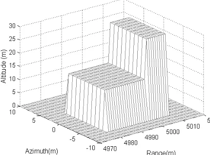
Here, we suppose that there are two cube buildings located at the scene. One building with altitude 15 m is located at−5 to 5 m in the azimuth direction and 4980 to 5000 m in the range direction. And the other building with altitude 30 m is located at−5 to 5 m in the azimuth direction and 5000 to 5010 m in the range direction. The position distributions of the two buildings are shown in Figure 2. For the sake of simplicity, we assume that there are only strong scattering centers in the roofs of the two buildings. From Figure 1, we can get that as the 3-D imaging coordinates for tomography SAR are presented in the azimuth, slant range and height directions, which are different from the ground coordinates (y, x,
z). Figure 3 shows the selected section of the imaging scene corresponding to the azimuth position 0 m. Figure 3(a) presents the selected section in the ground coordinates (x,z), and Figure 3(b) presents the selected section in the imaging coordinates (r,s).
49700 4980 4990 5000 5010 5020 5 10 15 20 25 30 35 Range(m) Al ti tu de (m )
7040 7045 7050 7055 7060 7065 -40 -30 -20 -10 0 10 20 30 40 Slant-range(m) Heig ht (m ) (a) (b)
Figure 3. The selected section of the imaging scene corresponding to the azimuth position 0m shown on (a) ground coordinates (x,z) and (b) imaging coordinates (r,s).
Slant range(m)
Heig
ht
(m
)
7040 7045 7050 7055 7060 7065 -40 -30 -20 -10 0 10 20 30 40 Slant range(m) Heig ht (m )
7040 7045 7050 7055 7060 7065 -40 -30 -20 -10 0 10 20 30 40
(a) (b)
Slant range(m)
Heig
ht
(m
)
7040 7045 7050 7055 7060 7065 -40 -30 -20 -10 0 10 20 30 40 Slant range(m) Heig ht (m )
7040 7045 7050 7055 7060 7065 -40 -30 -20 -10 0 10 20 30 40
(c) (d)
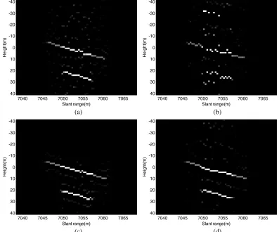
Figure 4. Comparison of the imaging sections of OMP and BOMP with different baselines. (a) OMP with eight baselines, (b) OMP with four baselines, (c) BOMP with eight baselines and (d) BOMP with four baselines.
the signal-to-noise ratio (SNR) is set to 5 dB. Figure 4 shows the selected slant range-height section of the final 3-D imaging result of tomography SAR corresponding to the azimuth position 0 m. Figures 4(a) and 4(b) show the 2-D images of the selected slant range-height sections obtained by OMP with eight and four baselines, respectively. Figures 4(c) and 4(d) present the 2-D images of the selected slant range-height sections obtained by BOMP with eight and four baselines, respectively. By comparing the
-50 -40 -30 -20 -10 0 10 20 30 40 50 0.1 0.2 0.3 0.4 0.5 0.6 0.7 0.8 0.9 1 Height(m) No rma liz ed in te ns it y
-50 -40 -30 -20 -10 0 10 20 30 40 50 0.2 0.3 0.4 0.5 0.6 0.7 0.8 0.9 1 Height(m) No rma liz ed in te ns it y (a) (b)
-50 -40 -30 -20 -10 0 10 20 30 40 50 0 0.1 0.2 0.3 0.4 0.5 0.6 0.7 0.8 0.9 1 Height(m) No rma liz ed in te ns it y
-50 -40 -30 -20 -10 0 10 20 30 40 50 0 0.1 0.2 0.3 0.4 0.5 0.6 0.7 0.8 0.9 1 Height(m) No rma liz ed in te ns it y (c) (d)
-50 -40 -30 -20 -10 0 10 20 30 40 50 0 0.1 0.2 0.3 0.4 0.5 0.6 0.7 0.8 0.9 1 Height(m) No rma liz ed in te ns it y
-50 -40 -30 -20 -10 0 10 20 30 40 50 0 0.1 0.2 0.3 0.4 0.5 0.6 0.7 0.8 0.9 1 Height(m) No rm al iz ed in te ns it y (e) (f)
imaging results, it can be seen that both OMP and BOMP provide good reconstruction in the case of eight baselines. However, when the number of baseline decreases from eight to four, image quality of OMP decays significantly, and it is almost impossible to achieve perfect recovery for OMP. Distinctively, the imaging result obtained by BOMP exhibits clear profile of the target even with only four baselines. In order to reflect detailed characteristics of the imaging results, the azimuth-slant range pixel located at (0, 7050) is extracted for individual analysis. Moreover, the multiple signal classification (MUSIC) algorithm is also utilized to verify the superiority of the proposed method. For the selected azimuth-slant range pixel, Figures 5(a) and 5(b) show the normalized backscattered intensity in the height direction obtained by MUSIC with eight and four baselines, respectively. Figures 5(c) and 5(d) show the normalized backscattered intensity in the height direction obtained by OMP with eight and four baselines, respectively. Figures 5(e) and 5(f) present the normalized height reconstruction results obtained by BOMP with eight and four baselines, respectively. With using neighboring pixels to estimate the covariance matrix in MUSIC algorithm, the estimate performance decreases with the decrease of the number of baselines. When the number of baselines reduces to four, the estimation error is hard to accept, as shown in Figures 5(a) and 5(b). Furthermore, the pseudospectrum obtained by MUSIC algorithm is not related to the signal power spectrum. That is to say, the peaks of the MUSIC pseudospectrum only denote the existence of the targets. The reflectivities of the targets should be estimated by the amplitude estimator. From Figures 5(c) and 5(d), it can be seen that as the number of baselines decreases, it is almost impossible to achieve perfect recovery for OMP method with only four baselines. However, as using neighboring pixels information in reconstruction, BOMP overcomes the imaging quality limitation imposed by the low number of baselines, which provide a better reconstruction quality than OMP and MUSIC, as shown in Figures 5(e) and 5(f).
5. CONCLUSIONS AND FUTURE WORK
In this paper, a novel imaging strategy capable of focusing tomography SAR data has been proposed. The principle behind the method is based on using neighboring pixels information in reconstruction, which can overcome the imaging quality limitation imposed by the low number of baselines. Raw data of tomography SAR in L-band was simulated, and the focused images were achieved by MUSIC, standard CS and the proposed method in the presence of additive gaussian noise. Simulation results have shown that it is almost impossible to achieve perfect recovery for MUSIC and standard CS with just few baselines. However, with using neighboring pixels information in reconstruction, the proposed method provides a better reconstruction quality.
In the future, we may focus on the following: (i) deducing the minimum baseline numbers and obtaining the optimal baseline distributions of tomography SAR; (ii) considering the adaptive selection method for the neighboring pixels; (iii) employing other parallel techniques to solve the imaging problem of tomography SAR, such as Bayesian optimization; (iv) applying graphic processing unit (GPU) technique to improve the computational efficiency.
ACKNOWLEDGMENT
This work was supported by the National Natural Science Foundation of China under Grant 61201390, the Key Scientific Research Project in Universities of Henan Province under Grant 16A510004, the Fundamental Research Funds for the Henan Provincial Colleges and Universities under Grant 2014YWQQ10, and the Plan for Young Backbone Teacher of Henan University of Technology and Henan Province under Grant 2015GGJS-038.
REFERENCES
1. Curlander, J. C. and R. N. Mcdonough, Synthetic Aperture Radar: System and Signal Processing, John Wiley & Sons, 1991.
3. Morrison, K., J. C. Bennett, and M. Nolan, “Using DInSAR to separate surface and subsurface features,”IEEE Transaction on Geoscience and Remote Sensing, Vol. 51, 3424-3430, 2013. 4. Barrett, B., P. Whelan, and E. Dwyer, “Detecting changes in surface soil moisture content using
differential SAR interferometry,” International Journal of Remote Sensing, Vol. 34, 7091–7112, 2013.
5. Reigber, A. and A. Moreira, “First demonstration of airborne SAR tomography using multibaseline L-band data,” IEEE Transaction on Geoscience and Remote Sensing, Vol. 38, 2142–2150, 2000. 6. Reigber, A., F. Lombardini, F. Viviani, M. Nannini, and A. Martinez del Hoyo,
“Three-dimensional and higher-order imaging with tomographic SAR: Techniques, applications, issues,” IEEE International Geoscience and Remote Sensing Symposium (IGARSS), 2915–2918, 2015. 7. Lombardini, F. and A. Reigber, “Adaptive spectral estimation for multibaseline SAR tomography
with airborne L-band data,”IEEE International Geoscience and Remote Sensing Symposium 2003, 2014–2016, Toulouse, France, 2003.
8. Lombardini, F., F. Cai, and D. Pasculli, “Spaceborne 3-D SAR tomography for analyzing garbled urban scenarios: Single-look superresolution advances and experiments,”IEEE Journal of Selected Topics in Applied Earth Observations and Remote Sensing, Vol. 6, 960–968, 2013.
9. Sauer, S., L. Ferro-Famil, A. Reigber, and E. Pottier, “Three-dimensional imaging and scattering mechanism estimation over urban scenes using dual-baseline polarimetric InSAR observations at L-band,”IEEE Transaction on Geoscience and Remote Sensing, Vol. 49, 4616–4629, 2011.
10. Lombardini, F., M. Pardini, and F. Gini, “Sector interpolation for 3D SAR imaging with baseline diversity data,”IEEE 2007 Waveform Diversity and Design Conference, 297–301, Pisa, Italy, 2007. 11. Lombardini, F. and M. Pardini, “First experiment of sector interpolated SAR tomography,”IEEE
International Geoscience and Remote Sensing Symposium, 21–24, 2010.
12. Fornaro, G., F. Serafino, and F. Soldovieri, “Three-dimensional focusing with multipass SAR data,” IEEE Transaction on Geoscience and Remote Sensing, Vol. 41, 507–517, 2003.
13. Candes, E. J., J. Romberg, and T. Tao, “Robust uncertainty principles: Exact signal reconstruction from highly incomplete frequency information,”IEEE Transaction on Information Theory, Vol. 52, 489–509, 2006.
14. Donoho, D., “Compressed sensing,”IEEE Transaction on Information Theory, Vol. 52, 1289–1306, 2006.
15. Chen, W. and I. J. Wassell, “Optimized node selection for compressive sleeping wireless sensor networks,”IEEE Transactions on Vehicular Technology, Vol. 65, 827–836, 2016.
16. Zhang, Y., S. Wang, G. Ji, and Z. Dong, “Exponential wavelet iterative shrinkage thresholding algorithm with random shift for compressed sensing magnetic resonance imaging,” IEEJ Transactions on Electrical and Electronic Engineering, Vol. 10, 116–117, 2015.
17. Zhang, Y., Z. Dong, P. Phillips, S. Wang, G. Ji, and J. Yang, “Exponential wavelet iterative shrinkage thresholding algorithm for compressed sensing magnetic resonance imaging,”Information Sciences, Vol. 322, 115–132, 2015.
18. Zhu, X. X. and R. Bamler, “Tomographic SAR inversion by L1-norm regularization — The compressive sensing approach,” IEEE Transaction on Geoscience and Remote Sensing, Vol. 48, 3839–3846, 2013.
19. Budillon, A., A. Evangelista, and G. Schirinzi, “Three-dimensional SAR focusing from multipass signals using compressive sampling,”IEEE Transaction on Geoscience and Remote Sensing, Vol. 49, 488–499, 2011.
20. Schmitt, M. and U. Stilla, “Compressive sensing based layover separation in airborne single-pass multi-baseline InSAR data,”IEEE Geoscience and Remote Sensing Letters, Vol. 10, 313–317, 2013. 21. Eldar, Y. C. and M. Mishali, “Robust recovery of signals from a structured union of subspaces,”
IEEE Transaction on Information Theory Vol. 55, 5302–5316, 2009.
22. Eldar, Y. C. and H. B¨olcskei, “Block-sparsity: Coherence and efficient recovery,” IEEE International Conference on Acoustics, Speech and Signal Processing, 2885–2888, 2009.
efficient recovery,”IEEE Transaction on Signal Processing, Vol. 58, 3042–3054, 2010.
24. Aguilera, E., M. Nannini, and A. Reigber, “Multisignal compressed sensing for polarimetric SAR tomography,”IEEE Geoscience and Remote Sensing Letters, Vol. 9, 871–875, 2012.
25. Fishler, E. and H. Messer, “Detection of signals by information theoretic criteria: General asymptotic performance analysis,” IEEE Transactions on Signal Processing, Vol. 50, 1027–1036, 2002.