BM3D Image Denoising using Learning-Based Adaptive Hard Thresholding

(1)

Scholarship@Western

Electronic Thesis and Dissertation Repository

12-10-2015 12:00 AM

BM3D Image Denoising using Learning-Based Adaptive Hard

Thresholding

Farhan Bashar

The University of Western Ontario

Supervisor

Dr. Mahmoud R. El-Sakka

The University of Western Ontario Graduate Program in Computer Science

A thesis submitted in partial fulfillment of the requirements for the degree in Master of Science © Farhan Bashar 2015

Follow this and additional works at: https://ir.lib.uwo.ca/etd

Part of the Computer Sciences Commons

Recommended Citation Recommended Citation

Bashar, Farhan, "BM3D Image Denoising using Learning-Based Adaptive Hard Thresholding" (2015). Electronic Thesis and Dissertation Repository. 3359.

https://ir.lib.uwo.ca/etd/3359

This Dissertation/Thesis is brought to you for free and open access by Scholarship@Western. It has been accepted for inclusion in Electronic Thesis and Dissertation Repository by an authorized administrator of

(2)

HARD THRESHOLDING

(Thesis format: Monograph)

by

Farhan Bashar

Graduate Program in Computer Science

A thesis submitted in partial fulfillment

of the requirements for the degree of

Masters of Science

The School of Graduate and Postdoctoral Studies

The University of Western Ontario

London, Ontario, Canada

c

(3)

Image denoising is an important pre-processing step in most imaging applications. Block

Matching and 3D Filtering (BM3D) is considered to be the current state-of-art algorithm for

additive image denoising. But this algorithm uses a fixed hard thresholding scheme to

attenu-ate noise from a 3D block. Experiments show that this fixed hard thresholding deteriorattenu-ates the

performance of BM3D because it does not consider the context of corresponding blocks. In

this thesis, we propose a learning based adaptive hard thresholding method to solve this issue.

Also,BM3Dalgorithm requires as an input the value of the noise level in the input image. But

in real life it is not practical to pass as an input such noise level. In this thesis, we also

at-tempt to automatically estimate the level of the noise in the input image. Experimental results

demonstrate that our proposed algorithm outperforms BM3Din both objective and subjective

fidelity criteria.

Keywords: Image denoising, additive white Gaussian noise, Block Matching and 3D Fil-tering (BM3D), adaptive threshold, classification, random forest classifier, Peak

Signal-to-Noise Ratio (PSNR), Structural Similarity (SSIM) Index

(4)

At this happy moment, I would like to express my heartiest gratitude to the Almighty for the

strength, patience, intelligence and endless kindness he provided me with to finalize this thesis.

I am grateful to my honorable supervisor Dr. Mahmoud R. El-Sakka for his valuable

direc-tion, guidance, comments and encouragement throughout this work. It was an absolute honor

and privilege to work with such a modest and wise person like him. His wisdom and notable

thoughts have helped this thesis become an ultimate success. He redirected my view of thinking

to a progressive path every time I discussed my research problems with him. This dissertation

under his supervision will always be a remarkable experience in my life.

I would like to remember and broaden my delicate respect to all the professors of The

Univer-sity of Western Ontario who helped me through many courses to build my background for this

dissertation. Without their sincere care, the understanding of Image Processing fundamentals

would have been impossible for me.

Finally, I acknowledge the support of my friends, family members, my loving mother and

re-search group members throughout this long tiring period. Their inspiration and encouragement

strengthened me in my tough time to keep focused.

(5)

Certificate of Examination i

Abstract i

Acknowledgments ii

List of Figures vii

List of Tables xi

1 Introduction 1

1.1 Thesis Contributions . . . 2

1.2 Thesis Outline . . . 2

2 Image Denoising Background 4 2.1 Image Noise . . . 4

2.1.1 Additive White Gaussian Noise . . . 4

2.1.2 Salt-and-Pepper Noise . . . 5

2.1.3 Speckle Noise . . . 7

2.2 Image Denoising Techniques . . . 8

2.2.1 Spatial Domain Filter . . . 8

Mean Filter . . . 8

Median Filter . . . 9

Gaussian Smoothing . . . 9

(6)

Non-Local Means . . . 11

2D Adaptive Wiener Filter . . . 14

2.2.2 Frequency Domain Filter . . . 16

Low Pass Filter . . . 16

Wiener Filter . . . 16

2.3 Block Matching and 3D Filtering (BM3D) Algorithm and its Extensions . . . . 17

2.3.1 Algorithm . . . 18

BM3D First Step . . . 18

BM3D Second Step . . . 20

2.3.2 Extensions and Improvements . . . 21

2.3.3 Limitations . . . 23

3 Classification Background 25 3.1 Classification . . . 25

3.1.1 Classification Schemes . . . 25

Linear Discriminant Analysis (LDA) . . . 26

Native Bayes . . . 27

Support Vector Machine (SVM) . . . 28

K-Nearest Neighbors . . . 29

AdaBoost . . . 29

Random Forests . . . 30

Neural Networks . . . 32

4 Methodology 34 4.1 Main Idea of Proposed Algorithm . . . 34

4.1.1 Automated Noise Estimation . . . 34

4.1.2 Context-based Hard Thresholding . . . 35

(7)

4.2.1 Training . . . 36

Best Threshold Calculation . . . 38

Feature Generation . . . 39

Training Features . . . 41

4.2.2 Testing . . . 41

Noise Calculation and Classifier Selection . . . 41

Feature Vector Generation . . . 41

Classification . . . 42

Output Generation . . . 43

4.3 Parameters Selection . . . 43

4.3.1 Window Size for Noise Estimation (η×η) . . . 43

4.3.2 Threshold Range Selection . . . 43

4.3.3 Classifier selection . . . 45

5 Experimental Results and Analysis 47 5.1 Data Set . . . 47

5.2 Performance Measurement Metrics . . . 49

5.2.1 Objective Fidelity Criteria . . . 49

Peak Signal to Noise Ration (PSNR) . . . 50

Structural Similarity (SSIM) Index . . . 50

5.2.2 Subjective Fidelity Criteria . . . 51

5.3 Performance analysis . . . 51

5.3.1 Parameter Setting . . . 51

5.3.2 Performance analysis using PSNR and SSIM . . . 51

5.3.3 Subjective Comparison . . . 60

5.3.4 Intensity Profile . . . 73

(8)

6.1 Conclusion . . . 77

6.2 Future Work . . . 78

Bibliography 79

Curriculum Vitae 83

(9)

2.1 Distribution of Gaussian Noise . . . 5

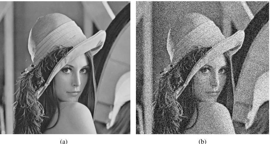
2.2 Example of Additive White Gaussian Noise. (a) Original Lena Image. (b)

AWGN added withµ=0 andσ=50 . . . 6

2.3 Example of pepper Noise. (a) Original Lena Image. (b)

Salt-and-Pepper added with density=0.25 . . . 6

2.4 Example of Speckle Noise. (a) Original Lena Image. (b) Speckle noise added

with mean=0 and variance=0.08 . . . 7

2.5 Performance of Anistropic diffusion (a) Original Lena image. (b) AWGN added withσ = 60 (PSNR=12.57) (c) Denoised image using Anisotropic dif-fusion, iteration=12 (PSNR=24.75) . . . 12

2.6 Performance of Non-Local Means (a) Original Lena image. (b) AWGN added

withσ= 60 (PSNR=12.57) (c) Non-Local Means denoised image (PSNR=27.25) 13

2.7 Performance of 2D Adaptive Wiener Filter (a) Original Lena image. (b) AWGN

added withσ =60 (PSNR=12.57) (c) Wiener2 denoised image (PSNR=24.35) 15

2.8 BM3D Block Diagram . . . 18

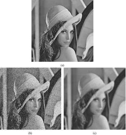
2.9 Performance of BM3D (a) Original Lena image. (b) AWGN added withσ=60 (PSNR=12.57) (c) Basic denoised image (PSNR=27.00) (d) Final denoised image (PSNR=28.27) . . . 22

3.1 Block diagram of a Classifier . . . 26

3.2 Layers of Neural Network . . . 32

(10)

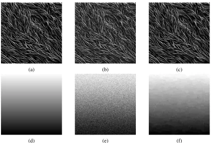
age. (b) AWGN added withσ = 60 (c) Best Denoised with threshold = 2.4 (PSNR=21.44, Original BM3D PSNR=20.35) (d) Smooth Image. (e) AWGN added with σ = 60 (f) Best Denoised with threshold = 3.1 (PSNR=36.95,

Original BM3D PSNR=35.29) . . . 37

4.2 Block Diagram of Proposed Algorithm . . . 37

4.3 Flowchart of Training . . . 38

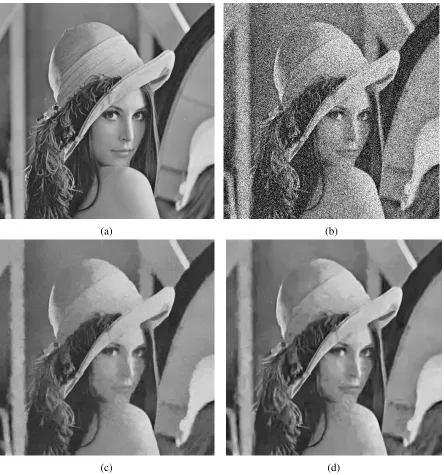
4.4 Performance of Denoised Image (a) Original Lena image (b) Noise image with σ=100 (c) Original BM3D Algorithm (PSNR=25.95) (d) Best BM3D Image (PSNR=29.21) . . . 40

4.5 Flowchart of Testing . . . 42

4.6 Comparing estimated noise with true noise based on different window size . . . 44

4.7 PSNR comparison for different threshold range . . . 45

4.8 Performance comparison using different classifiers . . . 46

5.1 Training Image set (Kodak Image set) . . . 48

5.2 Test Image set (Subset of BM3D Test Image set) . . . 49

5.3 Average PSNR comparison of test images . . . 52

5.4 Average SSIM comparison of test images . . . 53

5.5 Subjective Comparison of Lena Image (a) Original Lena Image. (b) AWGN added with σ = 100 (c) Denoised Image using BM3D (d) Denoised Image using Proposed Method (e) Face Cropped from BM3D Output (f) Face cropped from Proposed Method Output . . . 61

5.6 Subjective Comparison of Man Image (a) Original Man Image. (b) AWGN added withσ= 100 (c) Denoised Image using BM3D (d) Denoised Image us-ing Proposed Method (e) Cropped texture region fro BM3D output (f) Cropped texture region from proposed method output . . . 62

(11)

added withσ= 10 (PSNR=12.57) (c) Denoised Image using BM3D (PSNR=35.93) (d) Denoised Image using Proposed Method (PSNR=37.22) . . . 63

5.8 Subjective Comparison of Lena Image (a) Original Lena Image. (b) AWGN

added withσ = 20 (c) Denoised Image using BM3D (PSNR=33.05) (d) De-noised Image using Proposed Method (PSNR=34.46) . . . 64

(12)

added withσ = 100 (c) Denoised Image using BM3D (PSNR=25.95) (d) De-noised Image using Proposed Method (PSNR=27.54) . . . 72 5.17 Image for Intensity Profile Calculation. Red Line shows the Scan Line taken

as input to Intensity Profile (a) Lena Image (b) House Image . . . 74

5.18 Intensity Profile for Lena Image at scan Line 100 (σ = 50) (a) Original Image (b) Noisy Image (c) Denoised by BM3D (Pearson correlation = 0.9836) (d) Denoised by Proposed Method (Pearson correlation= 0.9934) (e) Combining (a), (c) and (d) . . . 75

5.19 Intensity Profile for House Image at scan Line 100 (σ =50) (a) Original Image (b) Noisy Image (c) Denoised by BM3D (Pearson correlation = 0.9766) (d) Denoised by Proposed Method (Pearson correlation= 0.9908) (e) Combining (a), (c) and (d) . . . 76

(13)

4.1 Comparing estimated noise with true noise based on different window size . . . 44

4.2 PSNR comparison for different threshold range . . . 45

4.3 Performance comparison using different classifiers for testing set (Based on PSNR) . . . 46

5.1 Average PSNR comparison of test images . . . 52

5.2 Average SSIM comparison for test images . . . 53

5.3 Standard Deviation of PSNR for test images . . . 54

5.4 Standard Deviation of SSIM for test images . . . 54

5.5 Performance comparison of Lena image . . . 55

5.6 Performance comparison of Cameraman image . . . 55

5.7 Performance comparison of Barbara image . . . 56

5.8 Performance comparison of Boat image . . . 56

5.9 Performance comparison of Couple image . . . 57

5.10 Performance comparison of Fingerprint image . . . 57

5.11 Performance comparison of Hill image . . . 58

5.12 Performance comparison of House image . . . 58

5.13 Performance comparison of Man image . . . 59

5.14 Performance comparison of Peppers image . . . 59

(14)

Introduction

A digital image is defined as a two dimensional discrete function. The value of this function

at any particular point is called the gray level or intensity of the image at that location. For

gray-scale images, this intensity value is limited between 0-255.

During the image acquisition or the transmission processes, sometimes the image sensor

produces mechanical and electronic interference which generate some unexpected or random

brightness information, known as noise. For general purpose images, the noise may be

neg-ligible and often ignored. However, there are sophisticated imaging applications such as face

recognition, object tracking, medical imaging, satellite imaging and segmentation where even

the small amount of noise degrades the performance of these applications. Thus the need of

proper image denoising algorithm has grown with much interest. Image denoising is often

considered as an important pre-processing step for various imaging applications.

Currently there is a lot of image denoising algorithms present to reduce various types of

noise. Block Matching and 3D Filtering (BM3D) [1] is one such popular algorithm that reduces

Additive White Gaussian Noise (AWGN) [2] from digital images and is considered to be the

current state-of-art image denoising algorithm.

In terms of denoising performance, BM3D is considered to be the best denoising filter so

far. It exhibits remarkable results as compared to other existing methods. BM3D works in

(15)

two identical steps. In first step, it generates a basic estimate of the noisy image using hard

thresholding. Then in the second step, it generates Wiener coefficients from the basic estimated image and denoises the noisy image based on these coefficients.

Although BM3D achieves excellent performance in reducing additive white gaussian noise,

it posses some limitations as well. Our main study will focus on finding these limitation and

provide possible solutions for them. By solving these limitations we can achieve higher

de-noising performance than that of the original BM3D.

1.1 Thesis Contributions

The main contribution of our thesis is to improve the performance of BM3D and provide

solu-tions over the limitasolu-tions of BM3D. We will focus on the following points:

• BM3D algorithm relies on a user provided noise level for each noisy image, which is

not practical for real time systems. This noise level is very important for estimating

the denoised image. We will incorporate a noise level estimation mechanism without

hampering the performance to make this as an automated system.

• In BM3D algorithm, a hard thresholding is used for any block of the noisy image. We

will illustrate that this thresholding scheme depends on image block’s texture and noise

level. Tuning this threshold can improve the performance of the BM3D scheme. Thus we

will propose a learning-based adaptive hard thresholding mechanism where each block

utilizes different threshold based on it’s context.

1.2 Thesis Outline

We have formalized our thesis into five chapters including this introductory discussion as

(16)

(17)

Image Denoising Background

In this chapter, we will review different types of noise that affect digital images and existing image denoising techniques. We will explain thoroughly the current state-of-art denoising

algorithm and its limitations.

2.1 Image Noise

Noise is a random variation of brightness information in images. Usually noise is produced

by the sensor or circuitry of imaging devices, i.e., scanner or digital camera. There are many

variants of image noise. A brief introduction of some noise variants is given below.

2.1.1 Additive White Gaussian Noise

Additive noise refers to the noise signal which is independently added to the image signal. If

y(x) is a original signal wherex∈Xis a 2D spatial coordinate that belongs to the image domain

andη(x) is the noise signal, then the received signal can be represented as:

z(x)=y(x)+η(x). (2.1)

White noise is a random signal with a constant power spectral density, that means it has

(18)

uniform power across the frequency band [2].

Gaussian noise is a statistical noise having a probability density function equal to that of

the normal distribution. The probability density function of a Gaussian noise is [3]:

p(i)= √1 2πσe

−(i−µ)2

2σ2 . _(2.2)

Here i represents the gray level, µ the mean value and σ the standard deviation. Figure 2.1

shows the probability density function for Gaussian noise.

Figure 2.1: Distribution of Gaussian Noise

Thus, Additive White Gaussian Noise (AWGN) refers to the signal which is independent,

has constant power spectral density and follows Gaussian (normal) distribution. Figure 2.2

shows an example of applying additive white gaussian noise (using matlab imnoise function).

2.1.2 Salt-and-Pepper Noise

Salt-and-pepper noise or spike noise is kind of impulsive noise spreaded across the entire

im-age where the intensity of the affected pixel changes to minimum possible gray value (0) or maximum possible gray value (255). This type of noise can be caused by analog-to-digital

(19)

salt-(a) (b)

Figure 2.2: Example of Additive White Gaussian Noise. (a) Original Lena Image. (b) AWGN added withµ= 0 andσ =50

and-pepper noise over the Lena image. Popular salt-and-pepper noise reduction techniques are

Median Filter and Adaptive Median Filter [2].

(a) (b)

(20)

2.1.3 Speckle Noise

Speckle noise is an example of multiplicative noise which means, the unwanted random signal

(noise) gets multiplied with the original signal. Speckle noise usually found in Synthetic

Aper-ture Radar (SAR) or medical ultrasound and optical coherence tomography images. A generic

formula of speckle noise can be represented as:

z(x)=y(x)×η(x). (2.3)

Herey(x) is the original signal wherex∈Xis a 2D spatial coordinate that belongs to the image

domain and η(x) is the noise signal. Figure 2.4 shows an example of applying speckle noise

over the Lena image. Some of the popular speckle noise reduction techniques are Lee Filter

[5], Kuan Filter [6], Frost Filter [7] and SRAD [8].

(a) (b)

Figure 2.4: Example of Speckle Noise. (a) Original Lena Image. (b) Speckle noise added with mean=0 and variance=0.08

Since this thesis is focused on reducing additive white Gaussian noise, we will only focus

(21)

2.2 Image Denoising Techniques

Image denoising can be performed either in the spatial domain or in the frequency domain.

In spacial domain, denoising is done by applying filter directly on the intensity values of the

image. On the other hand, in frequency domain technique, an image is transformed into the

frequency domain and then the filtering operations are performed. The resulting denoised

signal is transformed back into the spatial domain.

2.2.1 Spatial Domain Filter

In spatial domain filtering techniques, an image is denoised based on the statistics of its spatial

information, i.e., the intensity values of the image. This class of image denoising is simple

be-cause there is no cost for domain transformation. Some of the popular spatial domain filtering

algorithms are discussed below.

Mean Filter

Mean filter is one of the simplest method for spatial image denoising. It reduces the amount

of intensity variation between one pixel and the next. In this method, a M × N window is

selected around a particular pixel and the arithmetic average of all the intensity values of the

neighboring pixel is calculated. This value is then replaced with the center pixel of that window

[2]. Thus that particular pixel gets the mean value of its neighborhood. This filter smooths the

image and reduces noise. Typically, the value of M× Nis 3×3, 5×5, 7×7 or 11×11. The

formula of mean filter is given below:

ˆ

I(x,y)= 1

MN X

x,y∈η

I(x,y) (2.4)

HereI(x,y) is the original pixel, ˆI(x,y) is the denoised pixel andηis theM×N local

(22)

Median Filter

Median filter is another simple image denoising method similar to mean filter. Instead of

taking the arithmetic mean around a center pixel, median filter takes the median among the

neighborhood pixels and replace the center pixel value with this value. Median filter is very

effective for images having salt & pepper noise. As any gray image contaminated with salt-and-pepper noise only have noisy pixels valued 0 and 255, taking median around the neighborhood

of a noisy pixel and replacing noisy pixel with the median value reduces the noise. But it also

smooths the edges. Median filter is further modified to adaptive median filter by changing the

window size based on image noise level [2].

Gaussian Smoothing

Gaussian smoothing operator is a 2-D convolution operator that is used to reduce noise. It is

similar to the mean filter, but it uses a different kernel that represents the shape of a Gaussian (bell-shaped). Equation (2.4) can be changed to Gaussian smoothing by including the Gaussian

kernel, as shown in the following equation.

ˆ

I(x,y)= 1

MN X

x,y∈η

G(x,y)×I(x,y), (2.5)

whereG(x,y) is the Gaussian kernel, as shown below:

G(x,y)= 1 2πσ2e

−x2+y2

2σ2 , (2.6)

whereσ2 is the variance.

Anisotropic Diffusion

In typical spatial domain image denoising techniques i.e, mean filter or Gaussian smoothing,

(23)

whether the pixel is from a smooth region or an edge. So, edges become blurred in these

methods. To avoid this problem, Perona and Malik [9] proposed an edge preserving image

denoising technique called Anisotropic Diffusion. The main idea of this technique is to first identify whether a pixel is from a smooth region or an edge and then denoise it. The authors

suggested that a smoothing algorithm should have the following criteria:

1. Causality: No spurious detail should be generated while passing from finer to coarser scales.

2. Immediate Localization:At each resolution, the region boundaries should be sharp and coincide with the “semantically meaningful” boundaries at that resolution.

3. Piece-wise Smoothing:At all scales, intra-region smoothing should occur preferentially over inter-region smoothing.

Based on the smoothing criteria, they proposed an algorithm for image denoising where

iter-ative Gaussian smoothing is applied, while preserving the edges. The main features of this

algorithm can be divided into two parts:

1. Using non-linear smoothing function instead of linear smoothing.

2. Using anisotropic diffusion instead of isotropic diffusion

Linear smoothing treats every pixel with the exact same convolution whereas non-linear

smooth-ing treats a pixel with varysmooth-ing intensity, dependsmooth-ing on its neighborhood qualities. In general, if

a pixel is part of an edge, then little smoothing is applied, otherwise full smoothing is applied.

To detect whether a pixel is a part of an edge, we need an estimation E, which is calculated

using the following equation:

(24)

where ∇I is the gradient of the image. Based on the estimation E, a coefficient c(x,y,t) is generated which will control how much smoothing is needed to apply.

c(x,y,t)=g(||E||) (2.8)

whereg(||E||) is a monotonous decreasing function. Perona and Malik proposed two variations

of this function:

g(||E||)= e−(||Ek||)2 (2.9)

and

g(||E||)= 1

1+(||E_k||)2 (2.10)

Anisotropic Diffusion algorithm for image denoising iteratively blurs an image by calculating the divergence of its gradient (Laplacian of the image). But instead of calculating the

Lapla-cian directly from the image, the coefficient c(x,y,t) is multiplied with the gradient and then divergence is calculated. At timet, the next blurring function is:

It+1 = It+λ[cN× ∇NI+cS × ∇SI+cE × ∇EI+cW× ∇WI] (2.11)

where 0≤ λ≤ 1/4 for the numerical scheme to be stable. N,S,E,W are mnemonic subscripts

for North, South, East and West. ∇I indicates the nearest neighbor difference between two pixels in a particular direction. Figure 2.5 shows the performance of Anisotropic diffusion.

Non-Local Means

Non-Local Meas (NLM) is one of the most successful spatial domain image denoising scheme.

It follows patch based denoising method. Instead of filtering a single pixel based on its

neigh-boring pixels, it works with patches within a defined window. In this algorithm, a block/patch is defined around a particular pixel, also referred to as the reference patch. A search window

(25)

(a)

(b) (c)

Figure 2.5: Performance of Anistropic diffusion (a) Original Lena image. (b) AWGN added with σ = 60 (PSNR=12.57) (c) Denoised image using Anisotropic diffusion, iteration = 12 (PSNR=24.75)

similar patches are given a weight based on its similarity with the reference patch. The center

pixel of the reference patch is then denoised by a weighted averaging using center pixels of the

similar patches [10, 11].

(26)

(a)

(b) (c)

Figure 2.6: Performance of Non-Local Means (a) Original Lena image. (b) AWGN added with

σ= 60 (PSNR=12.57) (c) Non-Local Means denoised image (PSNR=27.25)

denoised value is computed using the following equation.

NL[v](i)=X

j∈I

w(i, j)v(j) (2.12)

(27)

which arev(Ni) andv(Nj), respectively. The weight is computed as,

w(i, j)= 1

Z(i)e

−||v(Ni)−v(N j)|| 2 2

h2 (2.13)

HereZ(i) is a normalization constant andhis a smoothing kernel width which controls decay

of the exponential function. Figure 2.6 shows the performance of Non-Local Means algorithm.

Many improvements have been suggested on the Non-Local Means algorithm in past few

years. Recently, Rehman and Wang proposed SSIM-Based Non-Local Means Algorithm [12]

which uses SSIM [13] between two patches to calculate their similarity. This algorithm achieved

much improvement over the original Non-Local Means algorithm. Also there are many

vari-ants of Non-Local Means algorithm. Adaptive Non-Local Means [14], Non-Local Medians

[15] are popular ones. Maruf and El-Sakka introduced t-test in Non-Local Means for

reduc-ing feature space [16]. Alkinani and El-Sakka [17] applied Non-Local Means in stereo image

denoising.

2D Adaptive Wiener Filter

2D Adaptive Wiener filter or Wiener2 filter took the idea of Wiener filter and applied it in the

spatial domain. Basically it estimates the image noise and filters the image based on this noise

[18, 19].

At first 2D Adaptive Wiener filter estimates the local mean and variance around each pixel

respectively:

µ(a,b)= 1

MN X

x,y∈η

I(x,y) (2.14)

and

σ2₍_a_,_b₎₌ 1

MN X

x,y∈η

I2(x,y)−µ2(a,b), (2.15)

(28)

(a)

(b) (c)

Figure 2.7: Performance of 2D Adaptive Wiener Filter (a) Original Lena image. (b) AWGN added withσ=60 (PSNR=12.57) (c) Wiener2 denoised image (PSNR=24.35)

pixel-wise Wiener filter using these estimates, as shown in Equation (2.16).

ˆ

I(x,y)= µ+ σ

2₍_x,_y₎₋_v2

σ2₍_x,_y₎ (I(x,y)−µ(x,y)) (2.16)

(29)

the local estimated variance. The noise variance calculation is shown below:

v2 = 1 MN

X

x,y∈η

σ(x,y), (2.17)

whereσ(x,y) is the local estimated variance calculated from Equation (2.15). Figure 2.7 shows

the performance of 2D Adaptive wiener filter.

2.2.2 Frequency Domain Filter

Spatial domain filter work with the intensity of the image. In frequency domain filtering

tech-niques, the input image f(x,y) is transformed to frequency domain F(x,y) and then a filter

H(x,y) is used. The denoised signalG(k,l) = F(k,l)× H(k,l) is then inverse transformed to get back the output image.

Low Pass Filter

Low pass filter is one of the basic frequency domain filter. This filter allows to pass the signal

with frequencies lower than the cutofffrequency and attenuates signals with frequencies higher than the cutofffrequency. As a result, the output image is smoothed because edge information remains in high frequencies. Thus this filter is not an edge preserving filter. The low pass filter

can be represented, as shown below:

H(k,l)=

              

1, if√k2+_l2<_f cut−o f f

0, if √

k2+_l2>_f cut−o f f

(2.18)

Wiener Filter

Wiener filter is one of the most popular frequency domain filter. It tries to estimate the noise

from a degraded image and denoise it based on the estimation. The main objective of Wiener

(30)

Square Error or Least Square Error filter. If f is the uncorrupted image and ˆf is the noisy

image then the expectation of Wiener filter is to have minimum MSE between them.

e2 = E(f − fˆ)2 (2.19)

As Wiener filter works in frequency domain, the estimated signal after Wiener filtering is

ˆ

F(u,v).

ˆ

F(u,v)=

_H∗₍_u,_v₎

|H(u,v)|2+ Sn

Sf

G(u,v) (2.20)

Here H(u,v) is a degradation function e.g., Gaussian blur. H∗(u,v) is the complex conjugate

of the degradation function. Sn and Sf are power spectrum of noise and power spectrum of

uncorrupted image respectively. G(u,v) is the observation. Usually the notationK = Sn/Sf is

used asSn andSf are uniform.

2.3 Block Matching and 3D Filtering (BM3D) Algorithm and

its Extensions

In recent years Block Matching and 3D Filtering (BM3D) becomes the most popular image

denoising technique. Dabov et al. [1] first proposed the idea in 2006 [21] and explained it

thoroughly in 2007. The algorithm was then analyzed by Lebrun [22] and implemented an

open-source version of this algorithm. BM3D achieves excellent performance in reducing

Ad-ditive White Gaussian Noise(AWGN). It has achieved state-of-the-art denoising performance

in terms of both objective and subjective assessment. In this section, we study the algorithm of

(31)

2.3.1 Algorithm

BM3D follows the concept of patch-based denoising mechanism, first introduced in Non-Local

Means (NLM) algorithm [10]. BM3D also extended it by denoising an image using two

iden-tical steps. In first step, a basic estimate of the noisy image is generated. This basic estimate is

then passed to the second step to generate the final denoised image. The block diagram of this

algorithm is shown in Figure 2.8.

Figure 2.8: BM3D Block Diagram

Let us consider the noisy observation of a true signal y(x) is z(x) = y(x) + η(x) where

x∈Xis a 2D spatial coordinate that belongs to the image domain andη(x)∼ N(0, σ2_{) is white}

Gaussian noise of varianceσ2. After the first step, a basic estimation is ˆybasic_{and after second}

step the final estimation is ˆyf inal_{. In the following portions of this section, we study detailed}

description of these two steps.

BM3D First Step

The first step of BM3D is known ashard thresholdingstep because here a hard thresholding is

used to eliminate noise from the image. First, a block/patch is defined around a particular pixel, also referred to as the reference patch. A search window is also defined around the pixel where

similar patches to the reference patch are searched. As the initial image is noisy, calculating

similarity between noisy blocks may degrade the performance. So, first the blocks are filtered

(32)

Euclidean-distance between the reference block and each of the other blocks are calculated.

This similarity measurement is called d-distance. Equation (2.21) shows how the d-distance

between two blocks is calculated.

d(ZxR,Zx)=

Υ´(τht_2D(ZxR))−Υ´(τ

ht 2D(Zx))

(Nht 1)2

(2.21)

whereΥ´is the hard-thresholding operator andτht

2Ddenotes the normalized 2D linear transform.

Usingd-distance values, similar noisy patches are grouped together into a set,Sht

xR, as shown

below:

Sht_x_R =d(ZxR,Zx)≤ τ

ht

match, (2.22)

where the fixedτht

match is the maximum d-distance which is used for calculating similarity

be-tween blocks. From this set, the noisy blocks are grouped together into a 3D block which

we denoteZSht

xR. A 3D linear transform is applied on this 3D block and hard thresholding is

applied on the obtained coefficients, called collaborative filtering. This thresholding attenuates the noise. An inverse 3D transform is applied to get back to the spatial domain. Equation (2.23)

shows the block-wise estimation of a 3D block.

ˆ

Y_Shtht xR =τ

ht 3D

−1

(Υ(τht_3D(ZSht

xR))), (2.23)

whereΥis a hard-threshold operator and ˆYht

Sht_xR is stacked block-wise estimation of noisy blocks

in set ShtxR. The final step in the first step of BM3D is to aggregate all the estimated blocks

together. Each of the estimated sets contains a number of blocks and these blocks contains one

or more same pixel locations. That means, a single pixel can have more that one estimation.

So to get the final estimation a weighted averaging is applied on the estimations. The global

basic estimate ˆybasicis computed by a weighted average of the block-wise estimates ˆY_Shtht xR

(33)

below:

ˆ

ybasic=

P

xR∈X

P

xm∈Sht_x∈R

whtxRYˆ

ht,xR

xm (x)

P

xR∈X

P

xm∈Sht_x∈R

wht xRXxm(x)

, (2.24)

wherewhtxR is the weight of a group of block which is calculated by the Equation (2.25).

whtxR =

               1

σ2_NxR

ht

, ifNxR

ht ≥ 1

1 otherwise.

(2.25)

The basic denoised estimate of the noisy image is then passed to the second step of BM3D to

generate the final estimation.

BM3D Second Step

The basic estimate ˆybasic from the input image is assumed to be significantly attenuated. This

image is used in the second step as reference true noise free image of the original image.

Second step of BM3D is identical to the first step. At first the noisy blocks are grouped together.

But here instead of using the thresholding-basedd-distance, normalized squaredl2-distance is

used to find similarity between the basic estimated blocks. For any reference block, the basic

estimated blocks are stacked together in a set using:

Swie_x_R = ||yˆ

basic

xR −yˆ

basic xR ||

(N₁wie)2 ≤τ wie

match (2.26)

Lets denote ˆybasic_Swie_x

R as the stack of basic estimated blocks andZS wie_x

R as the stack of noisy blocks

from original image. Wiener shrinkage coefficients are generated by applying 3D transform on the basic estimated group using:

WSwie_xR =

|τwie 3D(ˆy

basic Swie_x

R)

|2

|τwie 3D(ˆy

basic Swie_x

R)|

(34)

whereσ2is the variance of the noisy image. The 3D transform coefficients of the noisy blocks are multiplied, element-by-element, with the Wiener shrinkage coefficients. This is called Wiener collaborative filtering, as shown in Equation (2.28). Inverse 3D transform is applied to

get the estimated pixel values.

ˆ

Y_Swiewie xR = τ

wie 3D

−1

(WSwie xRτ

wie

3D(ZSht_xR)) (2.28)

Here ˆYwie Swie xR

is the final block-wise estimation. These estimated blocks are then aggregated

to-gether to generate the final global estimated image ˆyf inal_{. Aggregation is done using:}

ˆ

yf inal= P

xR∈X

P

xm∈Swiex∈R

wwie xR Yˆ

wie,xR

xm (x)

P

xR∈X

P

xm∈Swie_x∈R

wwie xR Xxm(x)

(2.29)

wherewwie

xR is weight of a reference block’s group which is calculated as:

wwie_x_R = σ−2||WSwie xR||

−2

2 (2.30)

The performance of BM3D is better, compared to the previous denoising algorithms. Figure

2.9 shows the performance of BM3D.

2.3.2 Extensions and Improvements

BM3D achieves better Peak Signal-to-Noise Ratio (PSNR) as compared to any existing image

denoising methods. It produces significant better result than the previous state-of-art image

denoising algorithm, Non-Local Means (NLM). A number of improvements and extensions of

BM3D has been introduced and still work is going on to improve the performance of BM3D.

After proposing the original BM3D based on gray scale image denoising, Dabov et al.

ex-tended their work to color image denoising [23] and video denoising [24]. They also introduced

(35)

(a) (b)

(c) (d)

Figure 2.9: Performance of BM3D (a) Original Lena image. (b) AWGN added with

σ = 60 (PSNR=12.57) (c) Basic denoised image (PSNR=27.00) (d) Final denoised image (PSNR=28.27)

filtering is done on the PCA coefficients of 3D blocks. They also proposed a new method named BM4D which uses BM3D to filter volumetric data. Thus instead of having 3D blocks,

here each time 4D blocks of data are filtered [26].

(36)

-distance of BM3D’s first step . Here instead of using a single hard threshold, they adaptive

generate the threshold value by using the gradient of the block, the SSIM between two blocks

and the noise level. But they have achieved a little improvement over original BM3D.

Harold et al. [28] presented the idea of learning based image denoising. They used neural

network to train large datasets and used multi-layer perceptron (MLP) method to denoise an

image patch by patch. But for high textured noise, this method achieves less accuracy than

BM3D.

Mittal et al. [29] also adapted a machine learning technique to predict the parameters for

BM3D. In the second step of BM3D, the noise level of the image is used. They have generated

the value of this parameter using a natural science statistics (NSS) method. A training is applied

on huge datasets and using SSIM, the sigma value is predicted for test noisy image. This

method needs a lot of time for training but the improvement is still not up to the bound.

Hasan [30] proposed an adaptive edge-guided BM3D to improve the performance of BM3D

for higher noise levels. It detects a noisy pixel suing its neighborhood pixels statistics and uses

a pre-filter in the fist step of BM3D. It achieves a little improvement over BM3D for higher

noise levels but for lower noise levels the performance is same as the original BM3D.

Hasan and El-Sakka [31, 32] proposed a method for improving the result of BM3D by

op-timizing the wiener filter used in the algorithm. Instead of using MSE in the objective function

of the Wiener filtering step of BM3D, they have used SSIM. Thus the objective function of

Wiener function changed to maximizing the SSIM between the denoised and true image. This

method achieves comparatively better performance than other improvements mentioned above.

2.3.3 Limitations

Though BM3D is currently the state-of-art image denoising algorithm, it still has limitations

and the performance can be improved. We have studied the BM3D algorithm in detail and

identified the persisting limitations of this algorithm. Some of the limitations are reported

(37)

1. Noise Level: In the implementation of BM3D algorithm, we have found that the actual noise variance of the image is provided to the algorithm which is used in both first and

second step. In real time systems, the actual noise variance is not practical to be provided

as an input.

2. Fixed Hard Thresholding:In the first step of BM3D algorithm, a hard threshold is used to attenuate noise from the 3D blocks. This threshold is fixed for all the blocks. Using

fixed threshold value deteriorates the performance of this algorithm because for smooth

region and textured region thresholding value should not be the same.

3. Poor Performance for Higher Noise Levels: BM3D has poor performance in higher noise levels as compared to lower noise levels. It happens because of using fixed

param-eters. If the parameters can be made adaptive then for higher noise levels, it can achieve

better performance.

4. Parameterized Setup: Regardless the type of transform used in BM3D, it used a fixed set of parameter. But each transform has its own best parameter. Therefore using same

parameters for all kind of transform need to be reviewed to evaluate whether these

(38)

Classification Background

In our proposed method, we have used a classifier. Therefore this chapter discusses some of

the existing classification techniques.

3.1 Classification

Classification is the problem of identifying the category of a new observation on the basis

of a training set of data containing observations whose category is known. It is considered

an instance of supervised learning, where a training set of correctly identified observations is

available. An algorithm that implements classification is known as a classifier. This classifier is

a mathematical function which maps input data to a category. Figure 3.1 shows how a classifier

works.

3.1.1 Classification Schemes

Different algorithms of classification has been proposed over the past years [33]. These al-gorithms were proposed, based on solving particular classification problems. The popular

classifiers are Linear classifiers (i.e., Fisher’s linear discriminant, Logistic regression, Naive

Bayes classifier), Support Vector Machines, Quadratic classifiers, K-Nearest Neighbor,

(39)

Figure 3.1: Block diagram of a Classifier

ing, Decision Trees (i.e., Random Forest) and Neural Networks. In the following section, we

will provide brief description of some of these classifiers.

Linear Discriminant Analysis (LDA)

Fisher’s linear discriminant or generally known as Linear discriminant analysis (LDA) is a

method to find a linear combination of features that characterizes or separates two or more

classes. LDA is used for dimensionality reduction also.

LDA seeks to reduce dimensionality while preserving as much of the class discriminatory

information as possible. Fisher suggested maximizing the difference between the means, nor-malized by a measure of the within-class scatter. LDA considers maximizing the following

objective:

J(w)= w

T

SBw

wT_S

ww

(3.1)

whereSB is the between classes scatter matrix andSwis the within classes scatter matrix. The

definition of these matrices are:

SB =

X

c

(µc− x¯)(µc− x¯)T (3.2)

SW =

X

c

X

i∈c

(xi−µc)(xi −µc)T) (3.3)

(40)

are used for classification. LDA performs very well if the features can be separated by a

linear hyperplane. Performance of LDA is not satisfactory if the discriminatory information of

features resides not in the mean but in the variance of the data.

Native Bayes

A Naive Bayes classifier is a simple probabilistic classifier based on applying Bayes’ theorem

(from Bayesian statistics) with strong (naive) independence assumptions. In simple terms, a

naive Bayes classifier assumes that the presence (or absence) of a particular feature of a class

is related to the presence (or absence) of any other feature [33].

Let T be a training set of samples, each with its own class labels. There are k classes,

C1,C2, ...,Ck. Each sample is represented by an n-dimensional vector, X = {x1,x2, ...,xn},

depictingnmeasured values of thenattributes,A1,A2, ...,An, respectively. Given a sample X,

the classifier will predict that X belongs to the class having the highest posteriori probability,

conditioned on X. That is, X is predicted to belong to the class Ci if and only if P(Ci|X) >

P(Cj|X) for 1 6 j 6 k, j , i. Thus the class that maximizes P(Ci|X) is predicted. The class

Ci for which P(Ci|X) is maximized is called the maximum posteriori hypothesis. By Bayes

theorem:

P(Ci|X)=

P(X|Ci)P(Ci)

P(X) (3.4)

Given data sets with many attributes, the naive assumption of class conditional independence

is made. This presumes that the values of the attributes are conditionally independent of one

another, given the class label of the sample. Mathematically it is:

P(X|Ci)= n

Y

k=1

P(xK|Ci) (3.5)

The probabilitiesP(x1|Ci),P(x2|Ci), ...,P(xn|Ci) is estimated from the training set.

A class prior may be calculated by assuming equiprobable classes, or by calculating an

(41)

distribution, one must assume a distribution or generate non-parametric models for the features

from the training set. The assumptions on distributions of features are called the event model

of the Naive Bayes classifier. For discrete features multinomial and Bernoulli distributions are

popular. If the training data contain a continuous attribute, Gaussian distribution works very

well [34].

Support Vector Machine (SVM)

Support Vector Machine (SVM) are supervised learning models with associated learning

algo-rithms that analyze data and recognize patterns, used for classification analysis. SVM performs

an implicit mapping of data into a higher dimensional feature space, and finds a linear

separat-ing hyper-plane with maximal margin to separate the data [33]. Given a trainseparat-ing set of labeled

examplesT =(Xi,li),i=1,2, ...,LwhereXi ={x1,x2, ...,xn}is a feaure vector andli ∈ {−1,1},

a new test dataxis classified by:

f(x)= sign(

L

X

i=1

αiliK(xi,x)+b) (3.6)

where αi are Lagrange multipliers of dual optimization problem, b is a bias or threshold

pa-rameter, and K is a kernel function [34]. The training samples xi withαi > 0 are called the

support vectors, and the separating hyperplanes maximizes the margin with respect to these

support vectors. Given a non-linear mapping function φthat transforms the input data to the

higher dimensional feature space, kernels have the formK(xi,xj)= φ(xi, φ(xj)). Of the various

kernels found in the literature, linear, polynomial and radial basis function (RBF) kernels are

the most frequently used.

SVM makes binary decisions and multi-class classification can be achieved by adopting the

one-against-rest technique, which trains a binary classifier for each class to discriminate one

(42)

K-Nearest Neighbors

K-Nearest Neighbors (KNN) algorithm is a non-parametric method used for classification. In

this algorithm, the training dataset is used only to populate a sample of the search space with

instances whose class is known [33]. No actual model or learning is performed during this

phase. When an instance whose class is unknown is presented for evaluation, the algorithm

computes itsk closest neighbors, and the class is assigned by voting among those neighbors.

Different distance metrics can be used, depending on the nature of the data. The Euclidean distance is typically used for continuous variables.

The training phase forKNN consists of simply storing all known instances and their class

labels. A tabular representation can be used, or a specialized structure such as a kd-tree. If

we want to tune the value ofkand/or perform feature selection, n-fold cross-validation can be used on the training dataset. The testing phase for a new instancet, given a known set I is as

follows:

1. Compute the distance betweentand each instance inI.

2. Sort the distances in increasing numerical order and pick the firstkelements.

3. Compute and return the most frequent class in theknearest neighbors, optionally

weight-ing each instance’s class by the inverse of its distance tot.

KNN algorithm is very simple in implementation and robust with regard to the search space;

for instance, classes don’t have to be linearly separable. The main disadvantage is that testing

is very expensive as the distance to all known instances need to be calculated. For large number

of dataset, it requires a lot time for classifying the data [33].

AdaBoost

AdaBoost, short for “Adaptive Boosting”, is a classification algorithm based the idea of

(43)

It is adaptive in the sense that subsequent weak learners are tweaked in favor of those instances

misclassified by previous classifiers. AdaBoost is sensitive to noisy data and outliers, however,

it can be less susceptible to the overfitting problem than other learning algorithms.

AdaBoost refers to a particular method of training a boosted classifier. It is an iterative

method, where initially equal weights are assigned to each training example. At successive

iterations, the weight of missclassified examples is increased. This forces the algorithm to

con-centrate on examples that have not been classified correctly so far. AdaBoost use the following

discriminant function:

g(x)=

T

X

t=1

αtht(x) (3.7)

where eachht is a weak learner that takes an object xas input and returns a real valued result

indicating the class of the object. The final classifier is the sign of the discriminant function.

Ff inal = sign[g(x)] (3.8)

AdaBoost can achieve similar classification results with much less tweaking of parameters or

settings over SVM. The user only needs to choose which weak classifier might work best to

solve their given classification problem and the number of boosting rounds that should be used

during the training phase.

Random Forests

Random forests are an ensemble of learning method for classification operated by constructing

a multitude of decision trees at training time and outputting the class that is the maximum votes

of the classes of the individual trees [33]. Random Forests grow many classification trees. To

classify a new object from an input vector, put the input vector down each of the trees in the

forest. Each tree gives a classification, and we say the tree votes for that class. The forest

chooses the classification having the most votes (over all the trees in the forest). Each tree is

(44)

1. If the number of cases in the training set is N, sample N cases at random - but with

replacement, from the original data. This sample will be the training set for growing the

tree.

2. If there are M input variables, a numberm<<M is specified such that at each node, m

variables are selected at random out of theMand the best split on thesemis used to split

the node. The value ofmis held constant during forest growing.

3. Each tree is grown to the largest extent possible. There is no pruning.

The forest error rate depends on two things:

1. The correlation between any two trees in the forest. Increasing the correlation increases

the forest error rate.

2. The strength of each individual tree in the forest. A tree with a low error rate is a strong

classifier. Increasing the strength of the individual trees decreases the forest error rate.

Random forest is one of the most efficient classifier where a large number of samples are used. Some features of this algorithm is [35]:

• It is excellent in accuracy among current algorithms.

• It runs efficiently on large data bases.

• It can handle thousands of input variables without variable deletion.

• It gives estimates of what variables are important in the classification.

• It generates an internal unbiased estimate of the generalization error as the forest building

(45)

Neural Networks

Artificial neural networks (ANNs) are a family of models inspired by biological neural

net-works and are used to estimate or approximate functions that can depend on a large number

of inputs and are generally unknown. Neural networks have been trained to perform complex

functions in various fields, including pattern recognition, identification, classification, speech,

vision abnd control systems. It can also be trained to solve problems that are difficult for human beings [33].

Neural networks are typically organized in layers. Layers are made up of a number of

in-terconnected nodes which contain an activation function. Patterns are presented to the network

via the input layer, which communicates to one or more hidden layers where the actual

pro-cessing is done via a system of weighted connections. The hidden layers then link to an output

layer where the answer is output as shown in Figure 3.2.

Figure 3.2: Layers of Neural Network

Most ANNs contain some form of learning rule which modifies the weights of the

con-nections according to the input patterns that it is presented with. In a sense, ANNs learn by

example as do their biological counterparts. Although there are many different kinds of learn-ing rules used by neural networks, this demonstration is concerned only with one; the delta

rule. The delta rule is often utilized by the most common class of ANNs called

backprop-agational neural networks (BPNNs). Backpropagation is an abbreviation for the backwards

propagation of error. Backpropagation performs a gradient descent within the solution’s vector

(46)

minimum is that theoretical solution with the lowest possible error.

Once a neural network is trained to a satisfactory level it may be used as an analytical tool

on other data. To do this, the user no longer specifies any training runs and instead allows

the network to work in forward propagation mode only. New inputs are presented to the input

pattern where they filter into and are processed by the middle layers as though training were

taking place, however, at this point the output is retained and no backpropagation occurs. The

output of a forward propagation run is the predicted model for the data which can then be used

(47)

Methodology

In Chapter 2, we have given background for different image denoising techniques. Also we have rigorously studied the BM3D Image denoising algorithm and pointed out some persisting

limitations of this state-of-the-art algorithm. In this chapter, we will first try to find solutions of

these limitations and then propose a new algorithm. Our proposed algorithm need a classifier.

We have reviewed some of the classifers in Chapter 3.

4.1 Main Idea of Proposed Algorithm

The BM3D has several limitations. In our thesis, we focus on two limitations: TheNoise Level

and Fixed Hard Thresholding (See Section 2.3.3). We have performed several experiments

to investigate these two limitations and developed our algorithm on those results. Below is a

detailed description of how we found our solution to these limitations.

4.1.1 Automated Noise Estimation

While using the authors’ provided Matlab software of BM3D, we have found that the true noise

level (standard deviation) of input noisy image is provided as input. Also, we have observed

that if the noise level is changed a little, the performance of the algorithm varies a lot. So,

(48)

we can say that the performance of the BM3D algorithm provided by the authors of BM3D

depends heavily on the value of the input parameter.

In our proposed algorithm, we created an automated noise estimation system where the

noise level of an input image is calculated first. We found that our noise level estimation is

very close to the actual noise level (see Section 4.3.1), hence eliminating such input without

degrading the performance.

For the noise level calculation, we have taken an idea from 2D adaptive Wiener filtering

(wiener2) algorithm [18, 19]. In this algorithm, image noise level is estimated based on the

local variance of the image. The local mean and variance around each pixel are calculated

using:

µ(a,b)= 1

MN X

x,y∈η

I(x,y) (4.1)

and

σ2

(a,b)= 1

MN X

x,y∈η

I2(x,y)−µ2(a,b), (4.2)

whereηis the N× M local neighborhood of each pixel in the imageI. The noise variance is

then calculated by averaging all the local estimated variance using Equation (4.3)

v2= 1 MN

X

x,y∈η

σ2₍_x_,_y₎_, _(4.3)

whereσ2₍_x,_y_{) is the local estimated variance calculated from Equation (4.2). From this noise}

variance given in Equation (4.3), we can calculate the standard deviation (σ) of the noisy

image. We have experimented using various neighborhood and found that 2×2 neighborhood

produces the closest estimation to the actual noise level.

4.1.2 Context-based Hard Thresholding

In the first step of BM3D algorithm, a hard thresholding is applied on the 3D noisy blocks

(49)

blocks (see Section 2.3.1).

Note that, the hard threshold operator Υis fixed for every block of the image.The BM3D used a fixed value,Υ =2.7. For images having noise level greater than 40 they have changed this value to Υ = 2.8. This threshold is used to attenuate the noise of corresponding block. But using a fixed level of threshold value is not quite a good choice, as blocks with different properties should have different threshold values.

We started our experiment to figure out whether different blocks should use different thresh-old values or not. First, we took two different images, one with high texture and the other with smooth region and then applied same level of noise to both of them. Next we applied the BM3D

algorithm to both of them using various threshold values and observed the best denoised

im-age. We observed that different threshold values are used to generate the best denoised image in each case. Figure 4.1 shows the result of this experiment. For a highly textured image, we

obtained the best denoised image for Υ = 2.4 and for a smooth image, we obtained the best denoised image with Υ = 3.1. Both of these denoise image showed significant improvement over the original BM3D where fixed threshold value is used. Similar experiments were also

performed using an image with various noise levels and it was observed that the best threshold

value also changes with the noise level.

4.2 Detailed Proposed Algorithm

Our proposed algorithm is divided into two main parts: trainingandtesting. A generic block

diagram of the algorithm is shown in Figure 4.2. A detailed description of the algorithm is

given below.

4.2.1 Training

(50)

(a) (b) (c)

(d) (e) (f)

Figure 4.1: Performance of BM3D with different Threshold value (a) High Textured Image. (b) AWGN added withσ=60 (c) Best Denoised with threshold=2.4 (PSNR=21.44, Original BM3D PSNR=20.35) (d) Smooth Image. (e) AWGN added withσ = 60 (f) Best Denoised with threshold=3.1 (PSNR=36.95, Original BM3D PSNR=35.29)

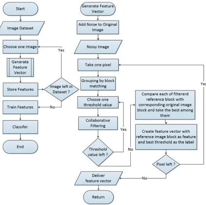
Figure 4.2: Block Diagram of Proposed Algorithm

their corresponding best threshold value as a label of that vector. The flowchart of this training

(51)

Figure 4.3: Flowchart of Training

Best Threshold Calculation

From the idea of context based hard thresholding, see Section 4.1.2, we know that different types of image blocks should have different threshold values. So, we conducted experiments on finding the best threshold value for any reference block.

1. To build a classifier for noise level n, we have applied AWGN withσ = nto all input images from the database.

(52)

the previous step. During collaborative filtering in the first step, we have used various

threshold values for each block. In our experiments, we have used 22 different threshold values, ranging from 1.7 to 3.8 with step size of 0.1.

3. The 22 denoised blocks (based on applying various threshold values) are compared with

the corresponding block in the original true image and the best among them is selected.

The comparison is done based on squared euclidean distance between these two blocks.

4. The threshold corresponding to the best denoised block is considered to be the best

threshold value of that particular block.

5. Every block and their best threshold value is stored in a matrix.

After taking all of the best denoised block during the collaborative filtering operation, we

found the generated output to be significantly better than the output of original BM3D

algo-rithm in terms of PSNR and visual quality. To assess the performance, we figured from the

results of experiment that the PSNR is improved by about 3 dB (on average) when the best

threshold is used, for a given noise level. Figure 4.4 shows the comparison among Best-BM3D

denoised image and original BM3D denoised image. From the subjective viewpoint, it is also

clear that using different threshold values for every block generates a better denoised image than the original BM3D algorithm. But in real life, the original image is not available, so we

need an intelligent algorithm to predict the best threshold values for any particular block. Thus

we will use various blocks and their best threshold values to train a classifier.

Feature Generation

1. For any input image, each of the image block is considered as a feature vector and their

corresponding best threshold value is considered as label of that feature.

2. Since we are considering blocks of size 7×7, thus each feature consists of 49 noisy pixel

(53)

(a) (b)

(c) (d)

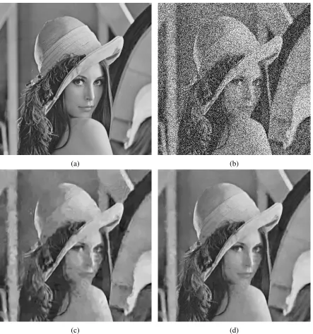
Figure 4.4: Performance of Denoised Image (a) Original Lena image (b) Noise image with

σ = 100 (c) Original BM3D Algorithm (PSNR = 25.95) (d) Best BM3D Image (PSNR = 29.21)

3. In an image of size M×N, a totalM× N feature vectors are generated, each of length

49 features.

4. To reduce memory and time complexities, we have only taken 10% of the total features,

(54)

Training Features

1. The generated features and their corresponding labels are used to train a classifier that

will be used in the next part of the algorithm.

In our experiment, we have used different classification techniques namely, Naive Bayes, SVM, K-Nearest Neighborhood and Random Forest to find out the best classifier for our algorithm.

Based on their performance we have decided to use Random Forest (RF) classification

algo-rithm.

4.2.2 Testing

In the testing phase, the classifier developed in the training phase is used to generate the

ap-propriate threshold to be used to denoise the input image. Figure 4.5 shows the flowchart for

testing. A detailed description of the testing phase is given step by step below.

Noise Calculation and Classifier Selection

1. From the test image, initial noise level is calculated using the algorithm described in

Section 4.1.1.

2. The noise is then rounded to the nearest multiple of 10. If the value is more than 100, it

is clipped at 100.

3. From the 10 trained classifiers, we choose our classifier based on the noise level.

Feature Vector Generation

1. The noisy input image is divided into several blocks of size 7×7. These 49 noisy pixels

are considered the feature vector of a single block.

(55)

Figure 4.5: Flowchart of Testing

Classification

1. The feature set is passed to the classifier.

2. The classifier will return the label of each feature vector.

(56)

Output Generation

1. The noisy image is filtered using BM3D image denoising algorithm with our predicted

noise level where in the collaborative filtering step, adaptive thresholding is applied.

2. All other operations will remain the same as in the original BM3D. After the second step

of BM3D, our final denoised image is generated.

4.3 Parameters Selection

In our proposed method, we have a few parameters which need to be adjusted. We have done

several experiments to find the best values for any particular variable. Below is a detailed

description of how these parameters are selected.

4.3.1 Window Size for Noise Estimation (

η

×

η

)

To find the best window size in our noise estimation step (see Section 3.1.1), we have

exper-imented on our training image set. This experiment is done in three steps. First, we applied

10 different noise levels to a black image and estimate the noise level. We found that the noise estimation method estimates the exact noise level. Then we estimated the noise level of a noise

free image and found that the noise level is close to zero. Then we applied 10 different noise levels to these images and estimated the noise level using Equation (4.3). We used different windows sizes to find out the best window size value. It is observed that for window size, 2×2,

our predicted noise level is almost close to the noise applied on these images. Table 4.1 shows

these results. Figure 4.6 shows the graph of the experimental results.

4.3.2 Threshold Range Selection

In our proposed method, we have used 22 predefined threshold values which are used in the

(57)

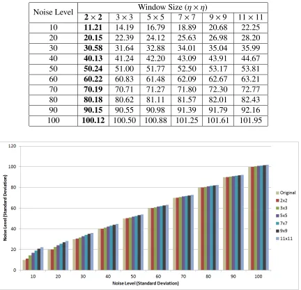
Table 4.1: Comparing estimated noise with true noise based on different window size

Noise Level Window Size (η×η)

2×2 3×3 5×5 7×7 9×9 11×11 10 11.21 14.19 16.79 18.89 20.68 22.25 20 20.15 22.39 24.12 25.63 26.98 28.20 30 30.58 31.64 32.88 34.01 35.04 35.99 40 40.13 41.24 42.20 43.09 43.91 44.67 50 50.24 51.00 51.77 52.50 53.17 53.81 60 60.22 60.83 61.48 62.09 62.67 63.21 70 70.19 70.71 71.27 71.80 72.30 72.77 80 80.18 80.62 81.11 81.57 82.01 82.43 90 90.15 90.55 90.98 91.39 91.79 92.16 100 100.12 100.50 100.88 101.25 101.61 101.95

Figure 4.6: Comparing estimated noise with true noise based on different window size

value for a particular block. We have performed experiments based on different threshold ranges to find the range which provides the best image. Table 4.2 shows the result of best

image based on different threshold ranges. It can be observed that if we increase the threshold range, the performance increases. But using 22 and 26 threshold values produces almost same

results. However, taking 26 threshold values increases the number of class labels. So, we have

taken 22 classes to reduce the time complexity. Figure 4.7 shows the graph representation of

(58)

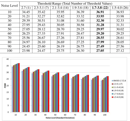
Table 4.2: PSNR comparison for different threshold range

Noise Level Threshold Range (Total Number of Threshold Values)

2.7 (1) 2.3-3.1 (7) 2.1-3.4 (14) 1.9-3.6 (18) 1.7-3.8 (22) 1.5-4.0 (26)

10 34.45 35.42 35.95 36.39 36.91 36.93

20 31.21 32.27 32.82 33.32 33.95 33.98

30 29.39 30.51 31.08 31.60 32.30 32.33

40 27.95 29.43 30.05 30.58 31.28 31.31

50 27.05 28.12 28.70 29.25 29.97 30.02

60 26.25 27.33 27.91 28.47 29.20 29.25

70 25.56 26.67 27.26 27.81 28.55 28.61

80 24.97 26.10 26.69 27.25 27.99 28.05

90 24.45 25.60 26.19 26.75 27.49 27.56

100 23.98 24.47 25.75 26.30 27.05 27.12

Figure 4.7: PSNR comparison for different threshold range

4.3.3 Classifier selection

Our proposed algorithm requires a classifier to train. For finding the best classifier, we have

tested our method using various classifiers, such as Naive Bayes, Support Vector Machine

(SVM), K-Nearest Neighbor, Decision Tree and Random Forest. Our experiment shows that

using Random Forests provides the best accuracy based on PSNR of the denoised image.

Fig-ure 4.8 shows the performance of average denoising result on our test images. The Best BM3D