Free Space Radiation Pattern Reconstruction from Non-Anechoic
Data Using the 3D Impulse Response of the Environment
Cesar Segura1, Wonil Cho1, Junghwan Jeon2, and Jinhwan Koh1, *
Abstract—Using impulse response with a 3D algorithm is a novel free-space radiation pattern reconstruction technique with accuracy greater than 1 dB in all antenna under test (AUT) azimuth and elevation angle orientations inside a non-anechoic environment. A quantitative comparison between impulse response with a 3D algorithm and impulse response with 2D, a previous technique, is performed using quantifiers. Benefits of the proposed 3D free-space radiation pattern reconstruction algorithm are single-frequency characterization and reuse of the 3D impulse response of the environment.
1. INTRODUCTION
An antenna radiation pattern is the directivity or gain with which an antenna transmits electromagnetic waves to the environment, and it is proportional to the quotient between the maximum radiated power of the antenna in a direction and the total radiated power [1]. Free-space radiation patterns are extracted in a semi-anechoic chamber, where reflected waves are suppressed by calculating spatial impulse response of the environment [2]. Conversely, in a non-anechoic environment, there are reflections, diffractions and scatterings that interfere with the antenna under test (AUT) signal [3–5]. There are optional facilities to the reverberation or non-anechoic environments where signal propagation interferes with Equipment under Test (EUT), and they are Open Area Test Sites (OATS), Anechoic Chambers (AC) and Transverse Electromagnetic (TEM) cells [6].
Antenna radiation pattern reconstruction techniques use measurements in a non-anechoic environment to estimate the free-space radiation through the use of an algorithm. The fast Fourier transform (FFT) technique analyzes signals during free-space time domain, which is the time from an electromagnetic wave’s transmission to its reception by an antenna. However, there is ambiguity in time boundaries [2]. Test zone field compensation reduces extraneous electromagnetic fields to obtain accurate gain measurements and states that a deconvolution-based technique limits extraneous field compensation and increases the measurement time and the equipment required [7]. Plane wave synthesis is a technique for near-field measurement of microwave antennas without an anechoic environment, and incorporates the principles of a planar scanning system to control the extent and direction of the plane-wave flow at the antenna and the production of negligible low-field regions in the non-anechoic environment [8]. The time reversal technique is a wave inverse problem in complex environments where diverging scatterings in a multipath environment convert into a converging wave focused on the AUT [9]. The oversampled Gabor transform (OGT) is a Gaussian windowed short time Fourier transform (WSTFT) applied to measurements performed in a semi-anechoic chamber to remove the reflected components and obtain free-space radiation pattern estimations with an accuracy of less than 1 dB [10].
Received 10 March 2018, Accepted 24 August 2018, Scheduled 5 September 2018
* Corresponding author: Jinhwan Koh ([email protected]).
1 Department of Electronic Engineering, ERI, Gyeong Sang National University, Jinju, Korea. 2 Department of Industrial
The impulse response technique is a deconvolution based method to reconstruct the free-space antenna radiation pattern from a non-anechoic data with an accuracy of 1 dB. Impulse response with 2D [2] limitation, to characterize non-anechoic environments of horizontal plane surfaces, is due to the rotation of the AUT only in the azimuth and not elevation domain. If reflections exist in 3D space (with elevation angle), the assumption in [2] does not hold, and the result becomes inaccurate. Therefore, in the impulse response with 3D, the AUT rotates in the azimuth and elevation domain to characterize vertical and horizontal surfaces in order to reconstruct the free-space 3D antenna radiation pattern.
The objective of this paper is to prove that an impulse response with 3D outperforms an impulse response with 2D. In the graphs showing the impulse response with 2D and 3D, radiation pattern reconstructions also include the free-space and non-anechoic data as references for comparison.
In Section 2, an explanation of the impulse response with 3D technique is given, and the antenna configuration system is described. In Section 3, modeling and simulation of numerical examples in the WIPL-D electromagnetic solver [11] is performed, and simulation data are processed using MATLAB with the proposed algorithm. Next, in Section 4, analysis and descriptions of graphs are given. Finally, in Section 5, results and contributions are presented.
2. THEORY
2.1. Impulse Response in 3D Space
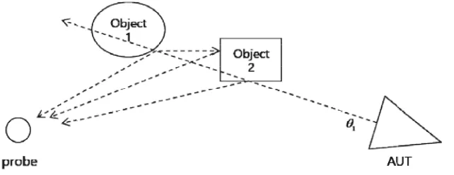
As shown in Fig. 1, the beam pattern at azimuth angle θ1 experiences reflection from Object 1 and
Object 2 located in the far field of the antenna, and multiple reflections between the two objects. This process can be characterized in the time domain by an impulse response and will be a unique feature with respect to every θi. Therefore, the non-anechoic environment can be modeled by a set of impulse responses in the time domain as a function of the spatial angles. These responses can easily be estimated by performing deconvolutions from first carrying out measurements in the environment of interest using two antennas whose ideal patterns are known. Once we get an estimate of the reference impulse response in time and angular domains, we can apply the reference responses to estimate patterns in anechoic environment of the antenna of interest by carrying out measurements in the same non-anechoic environment [2].
Figure 1. Multiple reflections to the probe.
The measured signal at the probing antenna along with the corrupting reflections can be represented as a convolution in time with the free space signal without any reflection and the impulse response of the AUT at an angle of θL can be written as
Pnon(θL, t) =Pfree−space(θL, t)⊗A(θL, t), (1)
or
Pnon(θL, f) =Pfree−space(θL, f)A(θL, f), (2)
where⊗denotes a time convolution, andPnon(θL, t) = time domain signal at the probing antenna from
the AUT in the presence of reflections for the angle θL, Pnon(θL, f) = frequency domain signal at the
space time domain signal without any reflection from the AUT for the angle θL, Pfree−space(θL, f) =
ideal frequency domain signal without any reflection from the AUT for the angleθL,A(θL, t) = impulse response of the environment with objects present when the AUT has a pencil beam pointing along the angleθL,A(θL, f) = frequency domain response of the environment with objects present when the AUT has a pencil beam pointing along the angle θL. Note thatA(θL, t) represents the contribution from the reflective stationary environments along the angleθL independent of the particular AUT.
In a real situation, the AUT would have a non-ideal beam pattern which may not be as sharp as a pencil beam. We define the impulse response of the environment with respect to such a non-ideal beam pattern of the AUT along the angle θL, as ˆA(θL, f). Then using Eq. (2) we have,
Pnon(θL, f) =Pfree−space(θL, f) ˆA(θL, f). (3)
Here, ˆA(θL, f) = frequency domain response with a non-ideal beam pattern of the AUT at the angle of
θL.
Now, we extend our discussion to 3D by introducing elevation ϕ. The free-space antenna coherent radiation pattern reconstruction technique utilizes measurements in a non-anechoic environment. The antenna configuration system elements are the AUT and probe antenna surrounded by metallic plates of finite conductivity. The AUT rotates in azimuth θand elevation ϕto the position (θ0, ϕ0). Depending
on the AUT geometry, the antenna either possesses or does not possess a pencil beam radiation pattern. The non-anechoic environment response when AUT does not possess pencil beam radiation pattern at frequencyf0 is
ˆ
A(θ, ϕ)|f=f0 =
Pnon(θ, ϕ)|f=f0
Pfree−space(θ, ϕ)|f=f0,
(4)
wherePnon(θ, ϕ)|f=f0 is AUT radiation pattern data in non-anechoic environment at frequencyf0, and
Pfree−space(θ, ϕ)|f=f0 is AUT radiation pattern measurement in free-space conditions at frequency f0.
Impulse response with 3D technique makes use of discrete convolution in azimuth θ and elevation ϕ angular domains in
P[θϕ]⊗A[θϕ] =∞
n=−∞
∞
m=−∞P[n,m]·A[θ−n, ϕ−m], (5)
where⊗denotes convolution;P[θ, ϕ] andA[θ, ϕ] are functions;nandmrepresent the indices of the data in the azimuth and elevation domain, respectively. When the AUT possesses a pencil beam radiation pattern the non-anechoic environment data are
Pnon(θ, ϕ)|t=t0 =A(θ, ϕ)|t=t0 ⊗Pfree−space(θ, ϕ)|t=t0, (6)
where Pfree−space(θ, ϕ)|t=t0 is the AUT free-space data at time t0, and A(θ, ϕ)|t=t0 is the environment
response at time t0 which can be extracted through deconvolution. The calculation of the environment
response when AUT has pencil beam radiation pattern requires result from Eq. (4) and is expressed by
A(θ, ϕ)t=t0⊗Pfree−space(θ, ϕ)t=t0 =F−1
ˆ
A(θ, ϕ)f=f0·Pfree−space(θ, ϕ)f=f0
, (7)
where ˆA(θ, ϕ)f=f0 is the non-anechoic environment response when AUT does not possess a pencil beam
radiation pattern at frequency f0; Pfree−space(θ, ϕ)|t=t0 and Pfree−space(θ, ϕ)|f=f0 are AUT data under
free-space conditions at timet0 and frequencyf0, respectively. Using the deconvolution in Eq. (7), the
environment response when the AUT possesses a pencil beam radiation pattern is
A(θ, ϕ)|f=f0 =F ⎧ ⎨ ⎩
F−1Aˆ(θ, ϕ)|
f=f0·Pfree−space(θ, ϕ)|f=f0
F−1[P
free−space(θ, ϕ)|f=f0]
⎫ ⎬
⎭, (8)
where ˆA(θ, ϕ)f=f0 is the non-anechoic environment response when AUT does not possess pencil beam
radiation pattern at frequencyf0, andPfree−space(θ, ϕ)|f=f0 is AUT data under free-space conditions at
frequencyf0. Using the deconvolution in Eq. (6), the AUT free-space 3D radiation pattern is expressed
as
Pfree−space(θ, ϕ)|f=f0 =F
⎧ ⎨ ⎩
F−1P
non(θ, ϕ)|f=f0
F−1A(θ, ϕ)|
f=f0
⎫ ⎬
wherePnon(θ, ϕ)|f=f0 is the data in the non-anechoic environment at frequency f0, andA(θ, ϕ)|f=f0 is
the environment response when the AUT possesses a pencil beam radiation pattern at frequency f0.
The procedure to reconstruct the antenna 3D free-space radiation pattern is as follows:
1. Obtain AUT free-space reference and non-anechoic reference data in the azimuth θ and elevation
ϕ. They are Pfree−space(θ, ϕ) and Pnon(θ, ϕ), respectively.
2. Calculate environment response when AUT possesses pencil beam radiation pattern using Eqs. (4) and (8) or (9).
3. Switching AUT to other types of antenna obtain non-anechoic environment dataPnon(θ, ϕ)|f=f0 in
the azimuthθ and elevationϕat frequency f0.
4. Reconstruct AUT free-space 3D radiation pattern Pfree−space(θ, ϕ) using (9).
Tests with a horn, a Yagi-Uda and a helical antenna as AUT and horn antenna as probe antenna are performed. The response of horn antenna is set as reference in order to reconstruct Yagi and helical antennas’ free-space radiation pattern. Two antenna configuration systems are presented with the only difference in the number of metallic objects.
3. NUMERICAL EXAMPLES
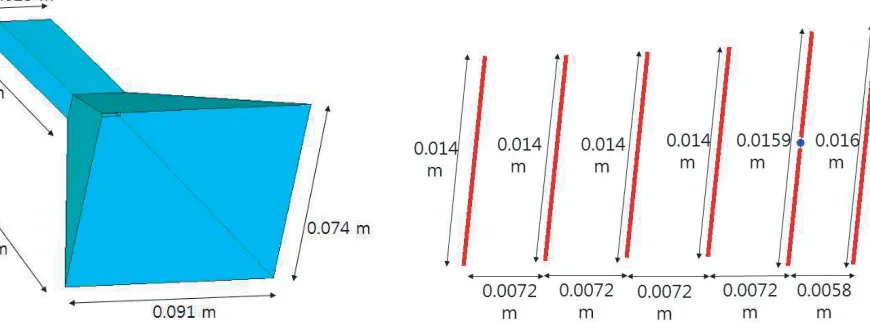
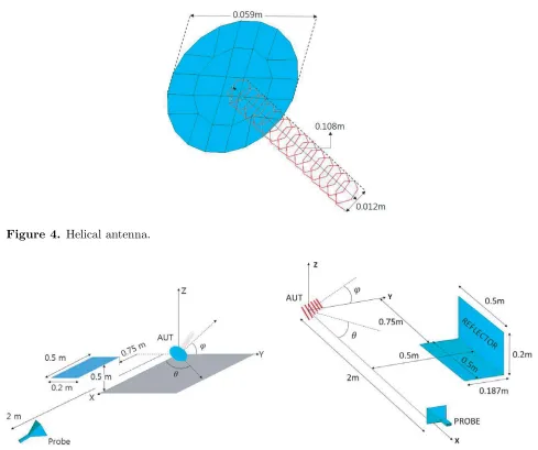
The antenna configuration system is stationary as the elements do not change in time with exception of AUT. We used WIPL-D software to show the availability of the proposed approach. The specifications of the computer used in the simulation are: CPU: E3-1231 v3, RAM: 16 GB, GPU: R9-280x. Most of the computation was performed within an hour per each angle. Horn, Yagi-Uda and Helical antennas are modeled and simulated as AUT or probe antenna at the frequency of 9 GHz in Figure 2, Figure 3 and Figure 4, respectively.
Figure 2. Horn antenna. Figure 3. Yagi-Uda antenna.
The antenna configuration systems in a non-anechoic environment are shown in Figure 5 and Figure 6. The AUT has a wide radiation pattern; however, metallic objects produce reflections, diffractions and scatterings, which interfere with the AUT signal. The AUT rotates in azimuth and elevation from−90◦ to 90◦ with an angle step of 5◦ to obtain an array of 37×37 data elements for each of the three AUTs.
Figure 4. Helical antenna.
Figure 5. Antenna configuration system using helical as AUT, horn as probe and metallic horizontal object.
Figure 6. Antenna configuration system using a Yagi antenna as the AUT, a horn antenna as the probe and metallic objects in vertical and horizontal planes.
with a distance of 0.5 m in theY axis. A comparison of the impulse response with 2D and 3D techniques is performed. Next, their normalized error, averaged in the elevation domain, is calculated using
E(θ) = meanϕ
|S21(θ, ϕ)−Sˆ21(θ, ϕ)
maxϕ|S21(θ, ϕ)|
(10)
where S21(θ, ϕ) is the free-space AUT radiation pattern, and ˆS21(θ, ϕ) is the AUT radiation pattern
reconstruction.
4. RESULTS
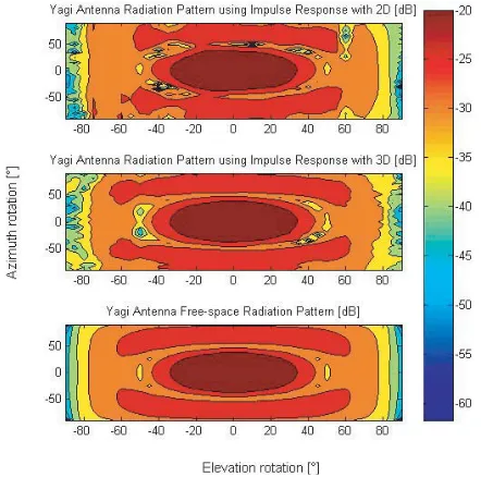
Next, in the contour graphs, fixing the elevation produces an antenna radiation pattern versus an azimuth range from −90◦ to 90◦. The first type is an amplitude pattern graph, which shows the magnitude in decibels versus an azimuth range from−90◦ to 90◦ at a fixed elevation. The second type is a phase pattern graph, which shows a phase in radians versus an azimuth range from−90◦ to 90◦ at a fixed elevation. All graphs are normalized with respect to the maximum value located at an azimuth of 0◦ in the center.
For the antenna configuration system in Figure 5, with a horn AUT as the reference, the Yagi and helical antenna radiation patterns are reconstructed using the impulse response with 2D and 3D
Figure 7. Yagi contour graph comparison between impulse response reconstructions with 2D, 3D and free-space radiation patterns from Figure 5.
Figure 8. Yagi contour graph comparison between impulse response reconstructions with 2D, 3D and free-space radiation patterns from Figure 6.
(a) (b)
techniques. Free-space and non data are included in the graphs of Figure 9 and Figure 10.
Figure 9(a) shows the magnitude of the reconstruction at 9 GHz and 20◦ elevation. An impulse response with 3D resembles a free-space pattern more than an impulse response with 2D. Figure 9(b) presents a comparison of the corresponding phases in radians. Figure 10(a) shows the magnitude of the reconstruction at 9 GHz and 0◦ elevation, and an impulse response with 3D reconstruction is closer to a free-space data than an impulse response with 2D reconstruction. Figure 10(b) presents the corresponding phase comparison.
For the antenna configuration system in Figure 6, with a horn AUT as the reference, the Yagi antenna radiation pattern is reconstructed using the impulse response with 2D and 3D techniques. Free-space and reverberation data are also included in the graphs of Figure 11.
Figure 11(a) shows the magnitude of the reconstruction of Yagi at 9 GHz and 30◦ elevation. The impulse response 3D reconstruction follows the free-space data closer than the impulse response with
(a) (b)
Figure 10. (a) Amplitude pattern of a helical antenna in dB at 9 GHz and 0◦ elevation. (b) Phase pattern in radians at 9 GHz and 0◦ elevation.
(a) (b)
2D reconstruction. Figure 11(b) presents a comparison of the corresponding phases.
Afterwards, a comparison is performed using the average normalized error for antenna radiation pattern estimation with 2D and 3D techniques in the antenna configuration system from Figure 5. Figure 12 shows the helical averaged elevation normalized error in decibels versus an azimuth range from −90◦ to 90◦. Figure 12 shows the error in the reconstruction of the impulse response with 2D and 3D with respect to the azimuth. The impulse response with 3D normalized error is lower than the impulse response with 2D in all orientations. Next, a comparison is performed using the average normalized error for antenna radiation pattern estimation with 2D and 3D algorithms in the antenna configuration system from Figure 6. Figure 13 shows the Yagi averaged elevation normalized error in decibels versus an azimuth range from −90◦ to 90◦.
Figure 12. Helical antenna reconstruction error at 9 GHz.
Figure 13. Yagi antenna reconstruction error at 9 GHz.
Figure 13 shows the error in the reconstruction of the impulse response with 2D and 3D with respect to the azimuth in a complex non-anechoic environment of vertical and horizontal metallic objects. The impulse response with 3D technique outperforms the impulse response with 2D technique at most azimuth orientations.
A quantitative comparison of results using averaged normalized error, maximum standard deviation and Euclidean distance metrics to provide indicators of the accuracy of the antenna radiation pattern reconstruction performance with the impulse response with 2D and 3D, is shown in Table 1 and Table 2. Table 1 presents a summary of the results of the antenna configuration system in Figure 5 using three metrics: the average of the averaged normalized error, maximum standard deviation and Euclidean distance. According to the three metrics, the Yagi antenna radiation pattern reconstruction with
Table 1. Antenna radiation pattern reconstruction metrics in Figure 5.
Antenna Metric Impulse Response with 2D
Impulse Response with 3D
Yagi
Eavg(%) 27.66 7.97
σmax 0.0063 0.0009
Euclidean 0.106 0.0227
Helical
Eavg(%) 34.668 26.47
σmax 0.0029 0.0014
Table 2. Antenna radiation pattern reconstruction metrics in Figure 6.
Antenna Metric Impulse Response with 2D
Impulse Response with 3D
Yagi
Eavg(%) 10.34 6.53
σmax 0.0014 0.0008
Euclidean 0.0361 0.0205
3D performance is superior to the reconstruction with 2D. The helical antenna radiation pattern reconstruction with 3D outperforms the reconstruction with 2D in the same fashion as the Yagi antenna. In Table 2, a summary of the Yagi radiation pattern error in Figure 4 demonstrates that the performance of the reconstruction with 3D is approximately 50% greater than the reconstruction with 2D for the three metrics, and the 3D Eavg of 6.53% is lower than 1 dB.
5. CONCLUSION
The impulse response method reconstructs the free-space radiation pattern using a single frequency. Based on quantitative results, the performance of the impulse response with 3D technique is superior to the impulse response with 2D technique in most if not all simulations. Based on qualitative results, the Yagi radiation pattern using an impulse response with 3D reconstruction resembles a free-space radiation pattern more than an impulse response with 2D reconstruction.
The main contribution of this work is a robust reconstruction technique that may be employed as a tool in a multipath reflection environment given that metallic objects disposed vertically and horizontally were correctly characterized. An impulse response with 2D technique can work in a non-anechoic environment where there are combinations of metallic objects’ azimuth and elevation orientations.
ACKNOWLEDGMENT
This work was supported by “Human Resources program in Energy Technology” of the Korea Institute of Energy Technology Evaluation and Planning (KETEP), granted financial resource from the Ministry of Trade, Industry & Energy No. 20174030201440) and National Research Foundation of Korea NRF-2016R1D1A1B03933848.
REFERENCES
1. Mahafza, B., “Radar antennas,” Radar Systems Analysis and Design Using MATLAB, 339–368, Chapman & Hall/CRC, 2000.
2. Koh, J., “Free-space radiation pattern reconstruction from non-anechoic measurements using an impulse response of the environment,” IEEE Transactions on Antennas and Propagation, Vol. 60, No. 2, Feb. 2012.
3. Loredo, S., M. R. Pino, F. L.-Heras, and T. K. Sarkar, “Echo identification and cancellation techniques for antenna measurement in non-anechoic test sites,” IEEE Antennas & Propagation Magazine, Vol. 46, No. 1, 100–107, Feb. 2004.
4. Fourestie, B., Z. Altman, and M. Kanda, “Anechoic chamber evaluation using the matrix pencil method,”IEEE Transactions on Electromagnetic Compatibility, Vol. 41, No. 3, 169–174, Aug. 1999. 5. Fourestie, B., Z. Altman, and M. Kanda, “Efficient detection of resonances in anechoic chambers using the matrix pencil method,” IEEE Transactions on Electromagnetic Compatibility, Vol. 42, No. 1, 1–5, Feb. 2000.
7. Black, D. and E. Joy, “Test zone field compensation,” IEEE Transactions on Antennas and Propagation, Vol. 43, No. 4, Apr. 1995.
8. Pereira, J. and A. Anderson, “New procedure for near-field measurements of microwave antennas without anechoic environments,” IEE Proceedings, Vol. 131, No. 6, Dec. 1984.
9. Punnoose, R. and D. Counsil, “Time reversal signal processing for communication,” SANDIA REPORT SAND 2011-7050, Sandia National Laboratories, Sep. 2011.
10. Fouristie, B. and Z. Altman, “Gabor schemes for analyzing antenna measurements,” IEEE Transactions on Antennas and Propagation, Vol. 49, No. 9, Sep. 2001.